Codeword Stabilized Quantum Codes:
Algorithm Structure
Abstract
The codeword stabilized (“CWS”) quantum codes formalism presents a unifying approach to both additive and nonadditive quantum error-correcting codes (arXiv:quant-ph/0708.1021). This formalism reduces the problem of constructing such quantum codes to finding a binary classical code correcting an error pattern induced by a graph state. Finding such a classical code can be very difficult. Here, we consider an algorithm which maps the search for CWS codes to a problem of identifying maximum cliques in a graph. While solving this problem is in general very hard, we provide three structure theorems which reduce the search space, specifying certain admissible and optimal additive codes. In particular, we find there does not exist any CWS code though the linear programing bound does not rule it out. The complexity of the CWS-search algorithm is compared with the contrasting method introduced by Aggarwal Calderbank (arXiv:cs/0610159).
I Introduction
Quantum error correcting codes play a significant role in quantum computation and quantum information. While considerable understanding has now been obtained for a broad class of quantum codes, almost all of this has focused on stabilizer codes, the quantum analogues of classical additive codes. Recently, a number of nonadditive quantum codes have been discovered, with superior coding parameters , the number of physical qubits being , the dimension of the encoded space , and the code distance [1, 2, 3]. These new codes have inspired a search for more high-performance non-additive quantum codes [4], a desire to understand how non-additive codes relate to additive codes, and how these may be understood through a cohesive set of basic principles.
A systematic construction, providing a unifying approach to both additive and nonadditive quantum error-correcting codes, has been obtained [1]. This codeword stabilized quantum codes (“CWS” quantum codes) approach constructs the desired quantum code based on a binary classical code , chosen to correct a certain error pattern induced by a self-dual additive quantum code which is without loss of generality, taken to be a graph state . The construction thus reduces the problem of finding a quantum code into a problem of finding a certain classical code. All previously known nonadditive codes [5, 6, 2, 7] with good parameters can be constructed within the CWS construction.
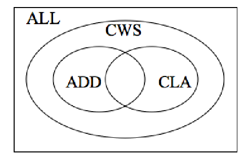
The natural challenge in these approaches is efficient identification of suitable classical codes, from which the desired additive and non-additive quantum codes can be constructed. It is apparent that due to the error pattern induced by the graph state , the binary classical code does not coincide with the usual binary classical code where the minimum Hamming distance is a more important code parameter – although interestingly, they do coincide in the special case where is an unconnected graph, so the family of CWS quantum codes includes classical (“bit-flip”) codes as depicted in Fig. 1.
The CWS construction, observing that a classical code correcting certain bit-flip error patterns gives rise to a quantum code, allows a natural encoding of the problem of finding a quantum code into an equivalent problem, of finding the maximum clique of an induced graph, called the CWS clique graph. The existence of such a mapping is not surprising, since maxclique is an NP-complete problem [8, 9], and thus can be used for a reduction from all unstructured search problems. In practice, many heuristic and randomized Clique solvers and SAT solvers have been developed, with reasonable run-times for small problem sizes. And since the search for CWS codes starts from a graph state , prior art in categorizing local Clifford (LC) orbits of those states [10, 11] helps simplify the problem. Nevertheless, without further simplification, a mapping of the CWS quantum codes search problem to maxclique leaves the problem unsolved, due to the exponential computational cost of solving maxclique. The real situation is even worse. For a general graph state, the search problem is NP-complete due to the reduction to maxclique. However, to search for all the quantum codes, we need to search for all graphs of vertices, which contributes a factor of order .
Here, we present an algorithm for finding CWS codes, based on a mapping to maxclique. We show that despite the exponential complexity of solving this cws-maxclique problem, the algorithm can be usefully employed to locate and identify a wide variety of codes, by taking careful steps to prune the search space. In particular, we show how the complexity cost can be reduced by using known graph isomorphisms and LC equivalences of graph states. We also present simplifying criteria for the search, arising from the structural properties of CWS codes. We prove three theorems limiting whether additive codes with optimal can be improved, or not, by the CWS construction. These theorems allow significant practical reduction of the search space involved in finding CWS codes using cws-maxclique. Furthermore, these theorems also indicate the existence of quantum codes outside of the CWS construction, as alluded to in Fig. 1.
We also compare and contrast the CWS codes with another framework (“AC06”) which was introduced independently [12] and is based on a correspondence between Boolean functions and projection operators. We interpret the AC06 framework to use a quantum state and a classical code, to generate the desired quantum code, but in a sense, it works in the reverse direction, starting from the classical code and obtaining the quantum state. We show how the AC06 Boolean function is the analogue of our classical code , up to a LC equivalence. This allows us to extend AC06 to degenerate codes, and to show that the AC06 framework can also be used to construct a search algorithm for new quantum codes, with comparable complexity to cws-maxclique.
II The cws-maxclique algorithm
The cws-maxclique algorithm is a procedure to search for a quantum error correction code , given a graph state which maps quantum errors in the Pauli group into binary error patterns, and a classical code , which corrects the error patterns. We present this algorithm below, beginning with a review of the basic definitions of CWS codes, proceeding to the details of the procedure, then rounding up with an evaluation of the computational complexity of the algorithm.
II-A Non-degenerate and degenerate CWS codes
The basic concepts and definitions of CWS codes are described in a previous paper[1], and may be summarized as follows. The standard form CWS code is fully characterized by a graph and a classical binary code , such that the corresponding CWS code may be denoted by the pair . We define
| (1) |
as the set of classical errors induced by quantum errors acting on the graph ; these are the errors that the classical code must detect. For each quantum error , it is sufficient to express in Pauli form as for some bit strings and . The mapping to classical error strings is
| (2) |
where is the th row of the adjacency matrix for , and is the bit of .
Using these definitions, the main theorem of the CWS code construction (Theorem 3 of [1]) may be given as:
Theorem 1
A standard form CWS code, for graph state and classical code , detects errors from if and only if detects errors from and in addition, for each ,
| (3) | |||||
| (4) |
where are codeword operators for from .
The case where for all is the non-degenerate case. For degenerate CWS codes, it will be useful to introduce a new set of classical bitstrings
| (5) | ||||
| (6) |
These bitstrings indicate codewords which are inadmissible, because they violate the condition given by equations (3) and (4) of Theorem 1. Specifically, fix a codeword , then for all we must have if . Writing , is not an admissible codeword if and . In other words, if a CWS code is degenerate, some low weight errors act trivially on the code space (i.e. ), and these errors must act trivially on each basis state generated from the graph state (i.e. ). describes basis states for which this is not the case.
II-B The cws-maxclique algorithm
Given a graph , the problem of finding a CWS code , which corrects for quantum errors , is reduced to a search for suitable classical codes. It is thus natural to ask how such classical codes can be found. One solution might be to use existing classical codes for this construction. However, that approach gives sub-optimal code parameters, due to the fact that should be able to detect errors of the highest weight of the induced error patterns in . This means that the classical code must have distance significantly greater than that of the corresponding quantum code , as shown in the following example:
Example 1
Let be an qubit ring graph. If is the set of single qubit Pauli , , and errors, then the induced classical errors are single, triple, and double bit flips respectively. Choosing the classical code to be a binary code results in a CWS code with parameters . However, also detects many additional errors which are unnecessary for this construction, such as all the one to six bit flip errors; only includes a subset of those errors.
This example motivates a search for specific classical codes which correct just the relevent errors for the CWS construction. However, classical coding theory provides no efficient, systematic constructions for codes that correct the potentially exotic error patterns involved in the CWS construction. On the other hand, finding a code with the best for given and is a problem which can be naturally encoded into an NP-complete problem such as maxclique. This classic approach has been employed, for example, to show that the classical code with has optimal parameters[13].
cws-maxclique is a mapping onto maxclique, of the problem of finding the CWS code with the largest possible dimension , for given parameters , , and graph . The cws-maxclique algorithm gives steps to solve this problem, and is given in detail in the Algorithm 3 box. It proceeds in several simple steps. The first step, Setup (Algorithm 1), finds the elements of and . The second step, MakeCWSCliqueGraph (Algorithm 2), constructs a graph, denoted as the CWS “clique graph,” whose vertices are classical codewords and whose edges indicate codewords that can be in the same classical code together. When searching for ordinary classical codes using an analogous procedure, the usual condition for joining two vertices by an edge is that the vertices are Hamming distance apart. In our situation, vertices are joined by an edge if there is no error induced by the graph state that maps one codeword to the other. Finally, an external subroutine findMaxClique is called; this routine is to employ known techniques to find the maximum clique in the CWS clique graph. The clique-finding subroutine is not specified here because there are many exact and heuristic techniques known in the community, for solving this classic NP-complete problem. Note that in the detailed description of the algorithms, two functions are used: , and its inverse, . Also, an error configuration is a list of ordered pairs where LOC is the coordinate of the affected qubit and TYPE is one of , , or .
II-C The complexity
cws-maxclique is not an efficient algorithm; the run-time is at least of order , because of the representation of the bit-string sets and . These are needed to specify the CWS clique graph, which has nodes. In principle, instead of storing all this in memory, the vertices and edges of this graph could be computed on the fly, during execution of the findMaxClique subroutine. However, these inefficiencies are not limiting factors, because of the even larger size of the search space involved in typical applications.
Typically, the goal is not to search for an optimal CWS code, given and , but rather, to determine if an code exists when and are fixed. When is fixed, finding a maximum clique is not necessary; rather, a clique of size is desired. There are such possible cliques. Checking whether a size subgraph of a CWS clique graph is a clique just requires checking if that subgraph is fully connected. Given an adjacency matrix for the CWS clique graph (and constant time access to the matrix elements), checking a subgraph takes order steps.
Searching over the space of all possible graphs involves searching a space of graphs with vertices, with a total of possibilities. Therefore, the complexity of searching for an CWS code is roughly
| (7) |
However, several practical improvements allow this search space to be pruned usefully. First, not all graphs need be considered; only those which are inequivalent under local Clifford (LC) operations need be checked. The LC orbits of graphs are well understood, and efficient algorithms exist to check for LC equivalence [10, 11, 14]. Therefore, the factor can be significantly reduced. A lower bound on the number of LC inequivalent graphs is given in [15], based on the number of non-isomorphic tree graphs, which roughly scales as . This reduction has played a key role in allowing us to employ the cws-maxclique algorithm on spaces with parameters up to and . However, no suitable upper bound is presently known, which would give a quantitative estimate of the extent of the search space reduction due to LC equivalence.
A second practical improvement comes from intrinsic properties of CWS codes, which rule out existence of codes of certain parameters, and relate the existence of certain parameter values with the existence of others. We will return to discuss these structure theorems in Section IV.
III Boolean functions and Classical Codes
The CWS construction unifies all known additive and non-additive quantum error correction codes of good parameters, including both degenerate and non-degenerate codes. An alternative framework (“AC06”) for non-degenerate codes, has been presented by Aggarwal Calderbank [12], based on a correspondence between Boolean functions and projection operators. Because AC06 implies a search algorithm for quantum codes which is in a sense the reverse of that employed above, in cws-maxclique, it is interesting to consider the differences.
In this section we study the relationship between AC06 and the CWS construction, by linking the AC06 Boolean function, which we interpret to specify a certain classical code, to the classical code used in the CWS construction. The components of the AC06 construction can be naturally associated with those of the CWS construction. In this way, we show that AC06 codes are spanned by a set of stabilizer states generated from a single state and a set of Pauli operators. Therefore, AC06 codes can be described completely, and in our opinion more transparently, as CWS codes.
That this identification between AC06 and CWS is natural was mentioned previously [1], but the transform required has not been presented before. It is well known that any stabilizer state is equivalent under some LC transform to a graph state. Thus, supposing that a local Clifford operation maps the AC06 stabilizer state to a graph state, it would be nice if this Clifford also described a transform from the Boolean function to the binary classical code of the CWS construction. Below, we show this mapping indeed exists, up to a technical subtlety with regard to the choice of the generating set for the stabilizer.
The AC06 framework is not entirely complete since degenerate codes cannot be described as presented in [12]. Degenerate codes may, in some cases, outperform the best known nondegenerate codes. Such an example may be provided by the code obtained by concatenating the code, since this is the best known code, it is degenerate, there is no known nondegenerate , and it has the highest possible minimum distance [16]. We take the constraints given for degenerate codes in the CWS construction and map these backwards to given new constraints for degenerate codes in the AC06 framework.
Given a complete AC06 framework which includes both non-degenerate and degenerate codes, we can then compare and contrast the computational cost of the CWS and AC06 approaches for seeking optimal parameter quantum codes. When the search goal is to find an optimal code for fixed and , the AC06 framework seems at first to involve a search over possibly Boolean functions, while cws-maxclique involves a search over possible graphs. This appears to give significant advantage to cws-maxclique. However, we find that with careful analysis of AC06, and extending it include degenerate codes, the two search algorithms have comparable complexity.
III-A AC06 quantum error-correcting codes are CWS codes
A -variable Boolean function is a mapping that maps a binary -vector to a bit . A Boolean function is nonzero if there exists some such that . We know that a Boolean function is naturally associated with a classical code
| (8) |
A nonzero Boolean function can be represented as
| (9) |
where and . The summation is taken to be modulo , i.e. XOR. The weight of a Boolean function is .
The complementary set of a nonzero -variable Boolean function is defined by
| (10) |
We know that the complementarly set is simply the set of vectors such that , i.e. it is the set of (classical) detectable errors of , since no codeword is mapped back into the code by .
Definition 1 (Definition 6 of [12])
Let and be projection operators on a Hilbert space with and . Then
- •
iff and
- •
is the projection of onto the span , the smallest subspace of containing both and
- •
is the projection of onto
- •
is the projection of onto
- •
.
Definition 2 (Definition 7 of [12])
Given an arbitrary Boolean function , the projection function is the expression in which in the Boolean function is replaced by the projection operator , multiplication (AND) in the Boolean logic is replaced by the meet operation in the projection logic, summation (OR) in the Boolean logic is replaced by the join operation in the projection logic, and the NOT operation in the Boolean logic is replaced by the not operation in the projection logic. Note that summation modulo (XOR) is replaced by the cooresponding operation in the projection logic.
Theorem 2 (Theorem 1 of [12])
If are pairwise commutative projection operators of dimension such that , , …, are all one-dimensional projection operators and is of dimension , then is an orthogonal projection on a subspace of dimension .
Let denote the concatenation of two -bit binary vectors and . The symplectic inner product of -bit binary vectors and is
| (13) |
The symplectic weight of a vector is the number of indices at which either or is nonzero. is defined by where equals if , if , if , and if and the associated projector is .
The next definition specifies the ingredients of an AC06 quantum error-correcting code (AC06 QECC). Theorem 1 of [12] defines a quantum code, but our definition of an AC06 QECC is based instead on Theorem 2 of [12], which provides sufficient conditions for the code to be an error-correcting code.
Definition 3 (AC06 QECC)
Let be an variable Boolean function and let be a list of the -bit column vectors of an matrix . An AC06 QECC with data is the image of the projector , where (i) the rows of are linearly independent with pairwise symplectic inner product zero and (ii) is associated to the th row of .
Theorem 3 (Theorem 2 of [12])
Let be the set of all -bit vectors of symplectic weight less than . An AC06 QECC with data is an quantum code if has weight and .
The main result of this subsection, stated and proven next, is that AC06 QECCs are CWS codes.
Theorem 4
An AC06 quantum error-correcting code is a codeword stabilized quantum code.
Proof:
Consider an AC06 QECC with data . The matrix , whose columns are , has linearly independent rows with pairwise symplectic inner products that are zero. Therefore, corresponds naturally to a group generated by pairwise commuting operators from the qubit Pauli group. Let be the state stabilized by for some -bit vector . A nonzero Boolean function can be represented as
| (14) |
which corresponds, in this case, to the projector
| (15) |
where and . The term projects onto the state , where , therefore
| (16) |
Hence, the AC06 QECC is spanned by a set of eigenstates of a stabilizer , each of which has a vector of eigenvalues given by a codeword in the inverted code , where indicates a eigenvalue for and indicates a eigenvalue for . To establish correspondence with a CWS code, we need to show that there is a mapping from -bit strings to Pauli operators such that . Indeed, there is a Clifford circuit that encodes and acts like for . Therefore, anticommutes with and commutes with all , . By this observation, the map
| (17) |
has the desired properties, and we obtain the set of CWS word operators by applying to each codeword in . Therefore, the AC06 QECC with data is associated with a CWS code (not in standard form) with stabilizer state corresponding to , classical code , and word operators . ∎
The mapping can be inverted to obtain data for an AC06 QECC from a CWS code as well. There is freedom in the choice of generating set for the stabilizer state in the CWS construction so it may be necessary to conjugate by a Pauli operator to fix the signs of the stabilizer generators to before mapping them to the column vectors .
Example 2
This detailed example demonstrates the mapping given in the proof of Theorem 4 from an AC06 QECC to a CWS code . The AC06 code is given by the boolean function
and the matrix
First, consider the boolean function . Indeed, is a function of variables and has weight . This can be seen by writing in the form
where equals if and if . The classical code is the set of -bit strings on which evaluates to , i.e. , , , , , and . Second, observe that the rows of are indeed linearly independent and pairwise orthogonal in the symplectic inner product. The rows of correspond to stabilizer generators , , , , and , respectively. These are the generators of the stabilizer for the state . The AC06 construction uses the fact that the projectors , , are pairwise commutative projection operators of dimension and , , …, are all -dimensional projection operators, so that is a projector onto a subspace of dimension (Theorem 1 of [12]), where the boolean operations are replaced by the operations defined in Definition 6 of [12]. Considering just the first term of , we see that
is a projector onto a stabilizer state where is a Pauli operator that commutes with and anticommutes with , i.e. . Notice that the partition of the generators into commuting and anticommuting sets is given by the first codeword of . The terms are combined using the operation , which equals when the projectors are pairwise orthogonal, as they are when and project onto stabilizer states. Therefore, where the are chosen to commute or anticommute with the generators of the stabilizer of according to the codewords of . We conclude that the AC06 code is a CWS code with stabilizer and word operators that correspond to the classical code specifying the generator’s signs for each basis state of the quantum code. We can arrange for the all-zeros codeword to be in by multiplying each word operator by (and, hence, adding to each codeword in ). This is a local operation, so the code parameters do not change.
III-B Mapping from AC06 to the standard form of CWS
Three distinct steps may be identified, in building a mapping between the AC06 code, and the CWS code in standard form,
| (18) |
First, is re-written as a stabilizer and a classical code , using standard definitions. The subscript on reminds us that the stabilizer is generated by the generators , where each generator corresponds to a row of . Second, a (non-unique) local Clifford transform turns into , leaving invariant. is a graph state with generators . Third, careful choice of appropriate generators turn the classical code into the used in the CWS construction. A fourth issue that arises is the limitation on needed to allow degenerate codes to be considered. These three steps and the degeneracy issue are discussed below, one at a time.
III-B1
We have already accomplished this step by way of Theorem 4, but we review it quickly to show the entire chain of steps to achieve standard form. The matrix describes the generators of a quantum stabilizer state, which we may denote as , when the left half is interpreted as describing Pauli terms, and the right half, Pauli terms, following the standard prescription[17]. Let the generators of this stabilizer be ; each generator corresponds to a row of . Let be the quantum state stabilized by .
The Boolean function defines a classical code, through its action on the bit strings ; explicitly, we may define
| (19) |
where denotes the complement of (needed because of how is defined in AC06, see Example 2).
In the CWS standard form, the all-zeros codeword is in the classical code , i.e. the state is in the code. This can be arranged by choosing one of the states in the code and applying to the whole code the local Pauli operation that maps to . Since this has no effect on the stabilizer , and the resulting code is locally equivalent to the original code, we now assume without loss of generality that contains the all-zeros codeword.
III-B2
The second step needed is an intermediate, but simple map, transforming into graph state form[14]. This can be done using Clifford operations on individual qubits (“LC transformations”). Importantly, though, we must also keep track of how transforms when the stabilizer is transformed, since is partially defined in terms of .
Let be the -qubit operation given by the tensor product of single qubit Clifford operations . When transformed by , the generators of the stabilizer map to become
| (20) |
where . Since also transforms to , it follows that the commutation relations of with are the same as between and . Thus, LC transformations leave unchanged, mapping into . Again, just as for , the subscript on reminds us that the generator of this graph state is , and originates from .
III-B3
The final step in transforming the quantum code into CWS form involves nailing down a degree of freedom which allows to be changed, without changing the stabilizer, or the quantum code specified. In particular, is dependent on the choice of generators for . Let be a binary valued, invertible matrix , which transforms a generator set into , where
| (21) |
We may keep track of this transform by rewriting as , though, of course, the stabilizer (and thus the corresponding graph) must be left unchanged when the generator set is changed. Upon this transformation by , the code must also be transformed, to keep the quantum code invariant. Specifically, if is written as a matrix, then:
Theorem 5
The quantum code is the same as the quantum code . That is, if the stabilizer generators are changed by , the code must also be transformed by matrix multiplication by .
Proof:
We have , and we want to calculate given by . Note
which gives . ∎
Essentially, this equivalence indicates that row reductions in the symplectic form of the stabilizer can leave the quantum code invariant, if the same row reduction is done to the binary code. Moreover, LC equivalence and the choice of generators of the graph state do not change the error correcting property of the quantum code. Thus, using a row reduction transform , and letting , we conclude that is a CWS code with dimension and distance identical to the original AC06 code .
It must be noted that the row reduction does change the errors (in terms of binary strings) detected by the classical code. More precisely, for a CWS code in the standard form that we have obtained from an AC06 code , we may define a corresponding in the language of AC06, by
| (22) | |||||
| (23) |
where is the identity matrix, and is the adjacency matrix of the graph .
The complementary set of the Boolean function is no longer the same as the the complementary set of the Boolean function , but they have same size due to the linearity of the transform relating and . Moreover, given quantum code distance , the set of induced classical error strings for is indeed the AC06 error set, specified as in Theorem 2 of [12], a subset of the complementary set of .
III-B4 Degenerate codes
The AC06 framework does not discuss how to allow for degenerate quantum codes, whereas the CWS construction includes these explicitly. The above mapping of AC06 to the standard form CWS codes applies only to non-degenerate codes, but the method indicates how degenerate codes can also be constructed using the AC06 framework, as follows. Specifically, one must appropriately constrain the Boolean function (ie ).
All degenerate quantum codes can be expressed using a certain form for , illustrated by the following. Consider a degenerate code of distance , given stabilizer . Define the set
| (24) | |||||
where gives the weight of the Pauli operator . If the rank of is , then independent elements can be chosen, such that generate , but are not in . According to the CWS construction described in the first step above, these generators imply a representation of a classical code with each codeword being for the first coordinates. In other words, stabilizes . Due to the one–to–one correspondence between and , this gives a structure for the values of , from which a search for degenerate codes can initiate.
III-C The algorithm complexity
Given the equivalence between AC06 and CWS codes, it is insightful to compare the algorithms implied by each for finding new codes. Both approaches construct a quantum code , but each analyze and calculate from different starting points. The search algorithm based on the CWS construction starts from the analysis of the structure of a given , takes a specification the desired properties of , and searches for a satisfactory , eg using the maximum clique algorithm. In contrast, the search algorithm based on the AC06 framework starts from the analysis of the structure of a given (ie, ), and searches for a stabilizer state which is LC equivalent to some graph state . This is why the two methods are in a sense, the mirror image of each other.
How do the computational complexities of the two approaches compare? AC06 implies an algorithm starting from a given classical code to find the quantum code . This suggests a need to consider different Boolean functions. In contrast, the cws-maxclique algorithm starts from possible graphs (or ideally, a smaller set of just the different ones).
However, this comparison is incomplete. In practice, if we really want to find an particular code, then there will be classical codes to look at, and for each code the AC06 algorithm needs to search for possible sets of strings. For a given classical code, to check whether a particular string is in the complementary set of the code takes steps. And to check whether a chosen set of strings gives a valid stabilizer state needs steps. Therefore, with the AC06 algorithm, the complexity of searching for an code is roughly
| (25) |
This is comparable but slightly worse than the result obtained for the cws-maxclique algorithm, in Eq. (7).
Some simplifications used in cws-maxclique may also apply to AC06; in particular, a reduction of the code search space due to LC invariance should be considered. In practice, in order to find all quantum codes , we only need to consider the codes equivalent under column reductions. For , this LC equivalence is the same as equivalence classification of all the binary linear codes, where . For fixed , the number of such codes is given by the Gaussian binomial factor [18]. Note this classification gives not only all the codes we need to start with, but also all the codes . For instance, the code , viewed by column, is an code , but not an code.
IV The structure theorems
The ability to search for CWS codes through solving the maxclique problem is unsurprising; any unstructured search problem can be reduced to an NP-complete problem. Thus, as it stands, the cws-maxclique algorithm presented in Section II is unsatisfactory (at least, for large cases), for the search space grows exponentially with the problem size . Moreover, as shown in Section III, the complexity of the AC06 algorithm is comparably bad, and is thus also unsatisfactory.
Since a major goal of the study of nonadditive codes is identification of codes with parameters superior to all possible additive codes, pruning the search space is worthwhile as a first step, before applying such brute-force search.
Is there hope? All nonadditive quantum codes with good parameters constructed so far have been CWS codes, as was shown in [1]. Also, very recently the CWS code was enumerated[3]; this code saturates the linear programing bound on code parameters. It thus seems that we should be optimistic about finding more CWS codes that outperform additive codes. We call an additive quantum code optimal if there does not exist any additive quantum code. One might hope that improved codes could be built from optimal additive codes, using the idea that these codes could be subcodes of larger (non-additive) CWS codes with superior parameters. If this were true, then a promising strategy would be to start with the optimal additive codes and try to increase the dimension.
This strategy leads to useful knowledge about the structural properties of CWS codes and reveals relations between codes with parameters and , where . These relations are especially interesting when given extra knowledge about the nature of the classical code employed in the construction. Surprisingly, we find that the low-dimensional CWS codes are actually additive. In particular, we find that all CWS codes are subcodes of some additive codes. Furthermore, we find restrictions on how optimal additive codes can and cannot be subcodes of larger CWS codes.
Before presenting these structure theorems, we review the relationship between the linearity of and the additivity of .
IV-A Linearity of and additivity of
Recall from Theorems 4 and 5 in [1] that the following facts are true:
Fact 1
If is a linear code (or equivalently, the word operators form a group), then is an additive code.
Fact 2
If is an additive code, then there exists a linear code and a graph , such that .
However, when is nonlinear, the question of whether is additive or not is completely open, since it may or may not be possible that is local unitary (LU) equivalent to some additive code.
The following example explicitly illustrates this possibility, by presenting two CWS codes: with nonlinear , and with linear . The two codes are LU equivalent to each other:
Example 3
Let
| (26) | |||||
| (27) | |||||
| (28) |
Note that is an additive code since the codewords of form a group under binary addition (it is thus a linear code). In contrast, since is nonlinear (its set of codewords are not closed under addition), is not LC equivalent to any additive code. Nevertheless, we can show that is LU equivalent to , by giving an explicit LU equivalence between the projectors into the two quantum code spaces, and . For this purpose, it is convenient to first transform by and disregard normalization factors, such that
| (29) | |||||
| (30) | |||||
From Theorem 4.2 of [19], LU equivalence need only consider where maps to and to . We find that , if is defined such that
| (31) | |||||
| (32) |
where is for and otherwise. The existence of this LU equivalence is unsurprising, since it is known [20] that any code is LU equivalent to the additive code.
In general, for a CWS code with a nonlinear , we cannot directly infer that is nonadditive. However, for fixed and , if we seek a code with optimal and only find codes with nonlinear , then we can conclude that nonadditive. Put another way, if we fix and , do an exhaustive search over all the graphs and classical codes, and only find quantum codes with nonlinear classical codes for the optimal CWS codes, then we can conclude that the optimal CWS codes we found are indeed nonadditive. This can be shown by contradiction: if is additive, then there exists some local unitary operation , where each is a single qubit operation, such that and is additive. Then, according to Fact 2, there exists a linear code and a graph such that .
IV-B Structure theorems
We now present and prove some structure theorems governing CWS codes, and provide several useful corollaries. Recall that we say an additive quantum code is optimal if there is no additive quantum code.
Our first theorem concerns CWS codes with dimension :
Theorem 6
All CWS codes are additive.
Proof:
By the CWS construction, an CWS code is spanned by basis vectors of the form , with word operators . However form a group. So according to Theorem 5 of [1] (or Fact 1), this CWS code is an additive code. ∎
A natural corollary of Theorem 6 is
Corollary 1
If an additive code of parameters is optimal, then there do not exist any CWS codes with parameters .
From corollary 1, it follows that the and nonadditive codes given in [21] and the code given in [19] are not local unitary (LU) equivalent to any CWS code, for they are not LU equivalent to any additive code. This implies that there exist codes that are outside the CWS construction, as was claimed in Fig. 1.
Now we present a theorem concerning CWS codes of dimension :
Theorem 7
Any CWS code is a subcode of some stabilizer code.
Proof:
By the CWS construction, any CWS code has the form with . Consider a new code with . From Theorem 1, it follows that detects errors in . To prove Theorem 7, we need to show that also detects those errors. It is clear that is a group with generators and that because . Therefore detects all of . Theorem 1 also requires that for each either or for all , commutes with . The latter constraint is satisfied by since . Finally, since is a group (and thus a linear code), according to Theorem 5 in [1] (or Fact 1), this CWS code is a stabilizer code. ∎
Two natural corollaries of Theorem 7 are:
Corollary 2
If an additive code of parameters is optimal, then there do not exist any CWS codes with parameters .
Corollary 3
There does not exist any CWS code, even though the linear programing bound does not rule out this possibility.
The two structure theorems above imply that CWS codes with parameters better than the optimal additive codes need dimension . We do know examples where , as the code [5] and the code [6] beat the optimal additive code with parameters [22].
Theorem 7 says that a CWS code of dimension is a subcode of some additive code with higher dimension. This invites a related question: when might an optimal additive code, of dimension , be a subcode of some CWS code of higher dimension? Unfortunately, we can show that in some sense, optimal additive codes cannot be subcodes of larger CWS codes, though we cannot show the impossibility in the most general setting, due to the fact that may be nonlinear even if a CWS code is additive.
Motivated by LU equivalences like the one demonstrated in Example 3, we show that if is a linear code, then an optimal additive code cannot be a subcode of any CWS code , where :
Theorem 8
Given a CWS code with parameters , if is a linear subcode of containing codewords, then there exists an additive code with parameters .
Proof:
By the CWS construction the classical codewords of can be arranged such that . From construct the linear classical code where but . Then is clearly an -qubit CWS code with codewords. It is an additive (stabilizer) code by Theorem 5 of [1] since is a group.
It remains to check the error-correction conditions. Theorem 1 ensures that detects errors in , i.e. no error can turn one codeword into another:
| (33) |
The same condition for is
| (34) |
where . Since the s are a group this reduces to
| (35) |
which is true, due to Eq.(33), and the fact that for all .
Theorem 1 also tells us that for all either (a) or (b) for all , . has the same graph as so whenever (a) is satisfied for it will be for . For (b) becomes for all and . Again, since for all , this is condition is met. ∎
Corollary 4
An optimal additive code (for which must be linear) cannot be extended to become a larger CWS code merely by adding codewords to .
Proof:
If the code could be extended in this way, by adding even just one vector, then there would exist an additive code with twice as many vectors and the same distance as the original code. This contradicts the statement that the original code is optimal. ∎
These structure theorems rule out certain strategies for finding non-additive codes with parameters superior to additive codes, but suggest other approaches. Since an additive code must have linear , Theorem 8 and corollary 4 tell us that in practice we cannot search for an CWS code just by adding codewords to . However, Example 3 hints that we may be able to shoehorn an optimal additive code into a CWS code with nonlinear , via some LU transform. This gives hope to a strategy of adding codewords to to search for CWS codes; such hope suggests that it is worthwhile both to further explore conditions under which two CWS codes can be linked by an LU transform, and to better understand the structural properties of CWS codes constructed from nonlinear codes.
V Discussion
cws-maxclique is an algorithm which may be usefully employed in the search for new quantum codes, both additive and non-additive, as described by the CWS construction. Given and , the algorithm can be used to search for an code , with a complexity which grows roughly as . In practice, by employing a number of search space simplifications, by pruning the set of graphs to explore based on LC equivalences, and by taking guidance from structural theorems about CWS codes, cws-maxclique and randomized variants of it have been used realistically[1] to explore codes with parameters up to and .
Many interesting questions arise in the construction of this algorithm. For example, it is likely that cws-maxclique can be improved with more memory efficient implementations; reductions to other NP-complete problems may also allow faster exploration of specific search spaces. Moreover, many of the simplifications used in cws-maxclique should also be applicable to the algorithm introduced by the AC06 framework; and in return, any code isomorphisms useful in simplifying AC06 should apply to cws-maxclique.
CWS codes present a rich structure, only partially described by the three structural theorems presented here. We believe that there are promising strategies for identifying new non-additive quantum codes based on expanding known additive codes, but such a strategy has to be executed carefully, because of limitations imposed by the theorems. Nevertheless, given an optimal additive code, there is hope for success with a strategy of adding codewords to to search for CWS codes, because of potential LU equivalences with some non-additive code. This hope suggests that it is worthwhile both to further explore conditions under which two CWS codes can be linked by an LU transform, and to better understand the structural properties of CWS codes constructed from nonlinear codes, so that more new quantum codes can be found. Indeed, one successful application of this idea results in new CWS codes encoding several more qubits than the best known codes [4]. It is an open question to determine if these nonadditive “quantum Goethals-Preparata codes” are LU equivalent to any additive quantum code.
Finally, despite the encompassing success of the CWS construction in describing all known non-additive codes with good parameters, we point out that there do exist codes, such as and codes, which are outside of the CWS construction. Since these codes are not LU equivalent to any CWS code, further new ideas will need to be developed to reach outside the stabilizer framework, for a complete understanding of quantum error correction codes.
Acknowledgments
JAS was supported by ARO contract DAAD19-01-C-0056, and AWC was supported in part by the JST CREST Urabe Project and an internship at the IBM T. J. Watson Research Center. We gratefully acknowledge comments and suggestions from V. Aggarwal and A. R. Calderbank.
References
- [1] A. Cross, G. Smith, J. Smolin, and B. Zeng, “Codeword stabilized quantum codes,” arXiv:quant-ph/0708.1201, 2007.
- [2] S. Yu, Q. Chen, C. H. Lai, and C. H. Oh, “Nonadditive quantum error-correcting code,” arXiv:quant-ph/0704.2122, 2007.
- [3] S. Yu, Q. Chen, and C. H. Oh, “Graphical quantum error-correcting codes,” arXiv:quant-ph/0709.1780, 2007.
- [4] M. Grassl and M. Roetteler, “Quantum goethals-preparata codes,” arXiv:quant-ph/0801.2150, 2008.
- [5] E. M. Rains, R. H. Hardin, P. W. Shor, and N. J. A. Sloane, “A nonadditive quantum code,” Phys. Rev. Lett., vol. 79, p. 953, 1997.
- [6] J. A. Smolin, G. Smith, and S. Wehner, “A simple family of nonadditive quantum codes,” Phys. Rev. Lett., vol. 99, p. 130505, 2007.
- [7] K. Feng and C. Xing, “A new construction of quantum error-correcting codes,” Trans. AMS, vol. 360, no. 4, pp. 2007–2019, 2008.
- [8] M. Sipser, Introduction to the Theory of Computation. PWS Publishing Company, 2005.
- [9] M. R. Garey and D. S. Johnson, Computers and Intractability: A Guide to the Theory of NP-Completeness. New York: W. H. Freeman and Company, 1979.
- [10] L. E. Danielsen and M. G. Parker, “On the classification of all self-dual additive codes over GF(4) of length up to 12,” J. Comb. Theo. A, vol. 113(7), pp. 1351–1367, 2006.
- [11] L. E. Danilesen, “On self-dual quantum codes, graphs, and boolean functions,” E-print quant-ph/0503236, 2005.
- [12] V. Aggarwal and R. Calderbank, “Boolean functions, projection operators and quantum error correcting codes,” arXiv:cs/0610159, 2006.
- [13] P. R. J. Ostergard, T. Baicheva, and E. Kolev, “Optimal binary one-error-correcting codes of length 10 have 72 codewords,” IEEE Transactions on Information Theory, vol. 45, pp. 1229–1231, 1999.
- [14] M. V. den Nest, J. Dehaene, and B. D. Moor, “Graphical description of the action of local clifford transformations on graph states,” Phys. Rev. A, vol. 69, p. 022316, 2004.
- [15] M. Bahramgiri and S. Beigi, “Graph states under the action of local clifford group in non-binary case,” arXiv: quant-ph/0610267, 2006.
- [16] M. Grassl, “Private communication,” http://www.codetables.de/, 2008.
- [17] M. Nielsen and I. Chuang, Quantum computation and quantum information. Cambridge, England: Cambridge University Press, 2000.
- [18] F. J. MacWilliams and N. J. A. Sloane, The Theory of Error-Correcting Codes. Amsterdam: North-Holland Publishing Company, 1977.
- [19] V. P. Roychowdhury and F. Vatan, “On the structure of additive quantum codes and the existence of nonadditive codes,” QCQC, pp. 325–336, 1998.
- [20] E. M. Rains, “Polynomial invariants of quantum codes,” IEEE Trans. Inf. Theo., vol. 46, no. 1, p. 54, 2000.
- [21] H. Pollatsek and M. B. Ruskai, “Permutationally invariant codes for quantum error correction,” Lin. Alg. Appl., vol. 392, pp. 255–288, 2004.
- [22] A. R. Calderbank, E. M. Rains, P. Shor, and N. Sloane, “Quantum error correction and orthogonal geometry,” Phys. Rev. Lett., vol. 78, pp. 405–8, 1997.