Voronoi Diagrams for Quantum States and Its Application to a Numerical Estimation of a Quantum Channel Capacity \jtitle \jauthor \eauthorKimikazu Kato \esupervisorHiroshi Imai \jsupervisor \supervisortitleProfessor {eabstract}In quantum information theory, a geometric approach, known as “quantum information geometry,” has been considered as a powerful method. In this thesis, we give a computational geometric interpretation to the geometric structure of a quantum system. Especially we introduce the concept of the Voronoi diagram and the smallest enclosing ball problem to the space of quantum states. With those tools in computational geometry, we analyze the adjacency structure of a point set in the quantum state space. Additionally, as an application, we show an effective method to compute the capacity of a quantum channel. In the first part of this thesis, we show some coincidences of Voronoi diagrams in a quantum state space with respect to some distances. That helps us to reinterpret the structure of the space of quantum pure states as a subspace of the whole space. More properly, we investigate the Voronoi diagrams with respect to the divergence, Fubini-Study distance, Bures distance, geodesic distance and Euclidean distance. For one qubit (or two level) states, the whole space is expressed as the Bloch ball. In the Bloch ball, we analyze the coincidence of the Voronoi diagrams in two different settings: 1)the diagram in pure states when Voronoi sites are taken as pure states and 2)the diagram in mixed states when sites are taken as pure states. We show that in both cases, all the diagrams coincide. This clear result is because of the symmetry specific for one qubit states. For three or higher level systems, we investigate the diagrams in pure states. The natural embedding of the quantum state space into a Euclidean space is no longer symmetric as in one qubit case. Consequently the coincidence of the Euclidean Voronoi diagram and the divergence-Voronoi diagram does not hold in a higher level system. However the coincidence of the divergence-, Fubini-Study- and Bures-Voronoi diagrams still holds. In the second part, we propose a method to compute a capacity of a quantum communication channel and show the result of the actual computation. We show that our method is sufficiently effective not only for one qubit states but for three level states. It is a practical application of the theoretical result shown in the first part; the theorems in the first part guarantee the correctness of the algorithm used in the second part. The algorithm uses Welzl’s algorithm to compute a smallest enclosing ball. Although the original algorithm introduced by Welzl is only for the Euclidean space, we show that the same method is useful for non-Euclidean space. We also implement the algorithm and experiment it to prove it is practical. {jabstract}
First of all, my Ph.D work is totally financially supported by Nihon Unisys, Ltd., which I belong to as an employee. I am very grateful to the company for providing me such an opportunity. I am also grateful to my adviser Hiroshi Imai for his advice and continuous support, and above all, for accepting me as a new member of his lab.
I thank coauthors of the papers which consists most of this dissertation. In particular, the very start of my research project is the discussion with Mayumi Oto. I owe her very much. I am also grateful to Keiko Imai and Jiro Nishitoba, who are also coauthors of the papers.
Discussions with my colleagues and related researchers are of course, essential to progress my work. Although I cannot list up all of them, an incomplete list includes François Le Gall, Jun Hasegawa, Masahito Hayashi, Tsuyosi Ito, Masaki Owari, Toshiyuki Shimono. I am grateful to them for their advice and fruitful discussions.
I am also thankful to Kokichi Sugihara, who advised me about figural presentation of some Voronoi diagrams; and Hidetoshi Muta, who provided some figures of Voronoi diagrams.
Last but not least, I would like to thank my family. I am specially thankful to my wife, Masumi Kato who supported my decision to go back to the university, and also grateful to my two daughters; Koko and Koto, who supported me by just being there.
Chapter 1 Introduction
In this chapter, we explain the background for our research and the summary of our contribution. Our contribution has mainly two aspects: computational geometry and quantum information theory.
In computational geometry, our contribution is shortly described as introduction of another Voronoi diagram with a distortion measure and an algorithm to solve the smallest enclosing ball problem in that measure.
In quantum information theory, we contribute to re-interpret the structure of a quantum state space to some extent, and proposed a practical algorithm to compute the capacity of a quantum channel.
We explain summarized background for topics related to our contribution. The explanation of the background is divided into two parts: one is about computational geometry and the other is about quantum information theory. Then, we explain the outline of the contribution of this dissertation, and show how this dissertation is organized.
1 Computational geometry
1.1 Voronoi diagrams
Voronoi diagrams and Delaunay triangulations have had an important role in computational geometry. Voronoi diagrams are not only useful for such applications as numerical calculation and visualization, but also useful for theoretical interpretation of a geometric object.
Practically, Voronoi diagrams are used in many fields such as geophysics, meteorology, astrology, geometric information system, city planning, and so on. Additionally, nowadays one of the most important applications of Voronoi diagrams is computer vision. In particular, because of the recent rapid development of computer graphics in entertainment media such as movies and games, Voronoi diagrams are getting more and more important. Other practical examples of applications are explained in [87].
A Voronoi diagram is a division of a space. The applications listed above all deal with a geometric space and need to divide it so that it can be computed in reasonable time. The essence of Voronoi diagrams can be explained as follows. Suppose that some points (which we call sites) are given and you want to divide the space into some regions so that each region expresses dominance of a point. If for any point in a region, the nearest site is the site included in the region in problem, then the division is called a Voronoi diagram. A Delaunay triangulation is a dual of a Voronoi diagram; for any two sites, draw a line between them if there is a Voronoi edge between them, and you obtain a Delaunay triangulation. Fig. 1 shows a example of Voronoi diagram and Delaunay triangulation.

As Voronoi diagrams used in the wider area, the more complicated diagrams with many Voronoi cells became needed and consequently, the robustness of the computation became emphasized. Actually, the general real world problems which needs Voronoi diagrams are badly positioned so that the resulting diagrams are degenerating. Degeneracy of Voronoi diagrams happens when the sites are cocircular. The evilness of degeneracy lies on the weakness for perturbation; only slight move of a site will change the topological position (See Fig. 2). In calculation in a computer where numbers are not expressed rigidly, this kind of evilness may cause inconsistent situation such as “A point is geometrically in a certain area, but topologically out of the area.” One off the researches to overcome this problem is by Sugihara and Iri [112, 113]. They achieved the robustness by focusing only on topologies and ignoring the geometries when computing about the relative position of edges. Thanks to those researches about the robustness of actual computation, now Voronoi diagram with billions of sites is shown to be computed. Isenburg et al. [58] showed an algorithm to calculate a tessellation of terrain data with a billion of triangles using some heuristics.

The significant application which emerged recently is fine art. Fritzsche et al. [36] proposed a algorithm to synthesize an authentic look mosaic structure from a picture. Sugihara [111] synthesize a artistic pattern. Since there is often a fractal structure behind a beauty in the nature, he proposed an algorithm to create a nature-like shape by combining Voronoi diagrams with fractal.
1.2 Generalized Voronoi diagram
In the original “normal” Voronoi diagrams, the sites are given as points and Euclidean distance is used to decide the dominance of each region. The generalization of Voronoi diagrams mainly goes into two ways: a) define a site as a set of point instead of one point, or b) use a general distance instead of the Euclidean distance.
In the direction to consider a general site, Voronoi diagrams for line segments were intensively researched from the late 70’s, by Drysdale and Lee [29], Drysdale [28], Kirkpatrick [72], Lee and Drysdale [73], Imai et al. [57], Sharir [106], Fortune [35], Yap [124], Clarkson and Shor [20], Goodrich et al. [38], Burnikel et al. [17], Rajasekaran and Ramaswami [98, 99], and Deng and Zhu [25]. The rather recent ones are Voronoi diagrams for circles or balls. Concerning the Voronoi diagrams whose sites are given as circles, Kim et al. [64, 65] proposed a algorithm which is robust even for the degenerating case.
Here, note that when we say “distance” in the context of Voronoi diagrams, it does not necessarily satisfy the axioms of a distance. In this dissertation, we use the word “measure”, or “pseudo-distance” in a confusing context.
Another direction is to use a general distance in a general space. One of the simplest in this direction is Voronoi diagrams for the weighted distance [87]. It means that each site has a weight and the distance is measured according to the weight. If is the weight for the site , then the multiplicatively weighted distance to the point is defined as . Fig. 3 shows an example of multiplicatively weighted Voronoi diagrams. The Voronoi edges for a multiplicatively weighted Voronoi diagram becomes a part of a circle, so called Apollonius circle.

The weighted distance is distorted to some extent, but it still based on Euclidean distance. Using more general distance, more distorted or sometimes pathological Voronoi diagrams can be obtained. For example, Onishi and Itoh investigated Riemannian Voronoi diagram [91]. In classical information theory, Onishi and Imai [89, 90] and Nielsen et al. [80] are for divergences. The detail of divergence Voronoi diagrams are explained in the next section.
The combination of the two directions described above can also be considered. Generalizing the way to decide the polygon mesh used in computer vision, Asano introduced an aspect-ratio Voronoi diagram and analyzed its computational complexity [6], and Asano et al. also introduced an angular Voronoi diagram [7]. In those diagrams, Voronoi sites are given as line segments and the distance is given as a visual angle or the aspect ratio of the triangle composed by a point and a line segment respectively. In both cases, the Voronoi edges are curves of degree three and the regions can be complicated; the region dominated by the same line segment can separated by points. Fig. 4 shows the example of angular Voronoi diagrams. Asano et al. also generalized those Voronoi diagrams to obtain an abstract notation of Voronoi diagrams and analyzed the characteristics of those diagrams [8].
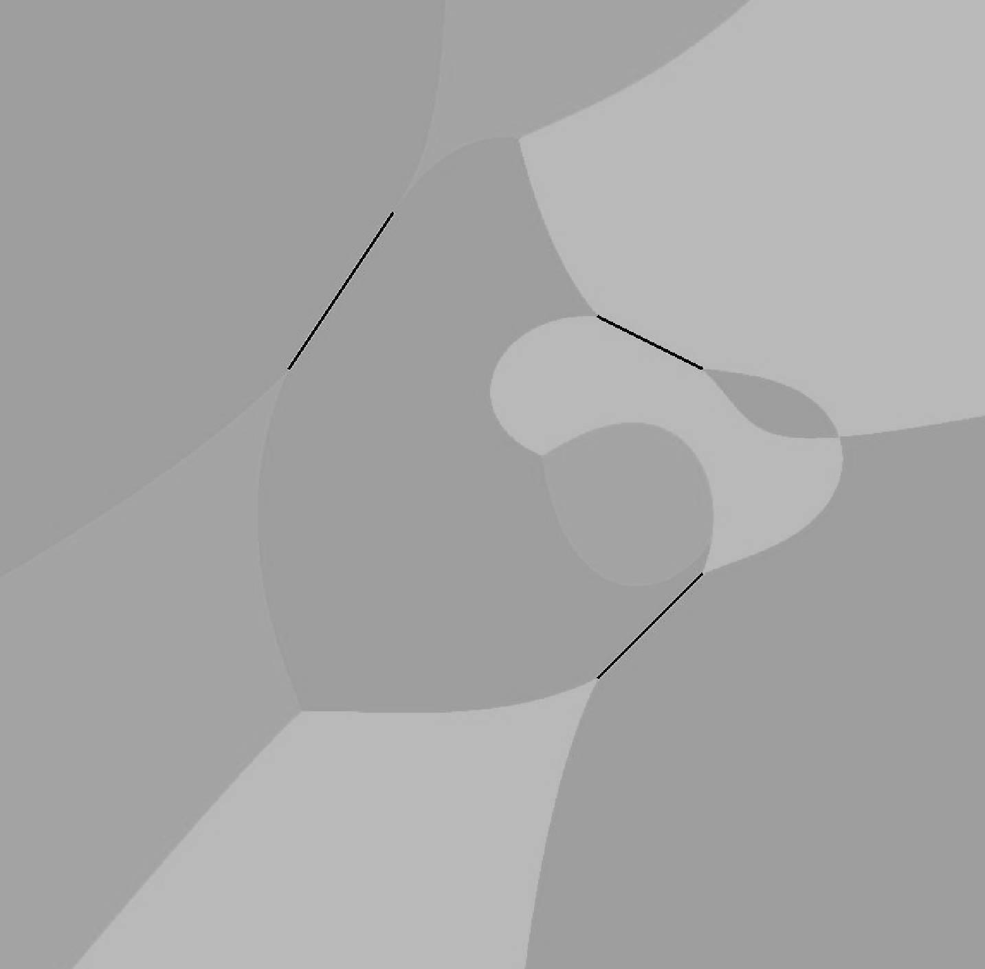
When we think about actual computation of those generalized distortion Voronoi diagrams, the arising problem is how we can achieve its robustness. Muta and the author analyzed the extended the notion of degeneracy of Voronoi diagrams from the viewpoint of the computational robustness [79]. The main discussion in the paper is about the conditions to make the number of crossing points of Voronoi edges jump with perturbation. It is only about angular Voronoi diagrams, but the concept of degeneracy in the paper is also applicable to general Voronoi diagrams, although there is only few attempt to actually compute the diagrams explicitly.
There are still other Voronoi diagrams with some “strange” measure spaces. In the book by Okabe et al. [87], many of them are introduced with analysis about their computational complexity.
1.3 Voronoi diagrams in classical and quantum information
Information theory is considered to have been founded by Shannon [105]. He showed the bound for the capacity of a channel by coding the source message of the channel. Its coding strategy is decided by the probabilistic distribution of the source message. Thus, information theory is mainly based on probability theory and statistics. The most important quantities used in this field are entropy, and Kullback Leibler divergence (or relative entroby). Kullback-Leibler divergence is defined as some kind of “distance” of two probabilistic distribution. Hence, geometry in information space can be considered but its structure is very distorted and far from intuition. Kullback-Leibler divergence does not satisfy the axioms of distance (so it is not a distance in a rigid sense); for example it does not satisfy the law of triangle inequity, or is not commutative either. However, its distorted and strange properties give a rich field of a research for computational geometry.
A computational geometric analysis was done by Onishi and Imai [89, 90], Onishi [88], and Sadakane et al. [101]. A Voronoi diagram and Delaunay triangulation are defined with respect to the Kullback-Leibler divergence, and are shown to be the extensions of the Euclidean counterparts. The Voronoi diagram is computed from an associated potential function instead of a paraboloid which is used in a Euclidean Voronoi diagram.
In the same line, Nielsen et al. [80] showed some properties of Voronoi diagram with respect to Bregman divergence, which is generalization of Kullback-Leibler divergence. Using the Voronoi diagram, Nielsen et al. [81] also showed that Welzl’s algorithm to solve the smallest enclosing ball problem is also applicable to Bregman divergence.
We extend the Voronoi diagram in classical information to the quantum world. In quantum information theory, there is a natural extension of the Kullback-Leibler divergence, and it is called a quantum divergence. We introduce a Voronoi diagram with respect to the quantum divergence, and analyze its structure. Additionally we consider other diagrams with respect to some distances. Comparing the diagrams, we can compare the structures of some distance spaces and consequently some problem concerning a certain distance can be replaced by another problem of another distance.
1.4 Smallest enclosing ball problem
The smallest enclosing ball is namely a problem to compute the smallest ball which contains given points. It has variety of applications; collision detection, facility location, automated manufacturing, and so on. It is a geometric problem but has some aspect of combinatorial optimization.
The first theoretically effective algorithm was given by Megiddo [77]. In spite of its astonishing idea of pruning-and-search, Megiddo’s algorithm was impractical because there is a big constant hidden behind a big-O notation. Welzl [121] gave the first practical algorithm based on Seidel’s randomized linear programming algorithm [104]. In these algorithms, however, the complexity is the exponential of the dimension. Eventually Matoušek et al. [75] discovered subexponential time algorithm. The most efficient algorithm known so far is Fischer and Gärtner’s algorithm [34]. They gave an -time algorithm. Fischer also implemented a program to compute the smallest enclosing ball problem as a part of CGAL [19].
Nishitoba et al. [83] connected this line of the research to the computation of the Holevo capacity in quantum information theory. He also shed light on combinatorial aspect of this problem. This direction is followed by Nishitoba [82] to analyze the combinatorial structure. Although Hayashi et al. had already showed the method using the smallest enclosing ball problem, they first mentioned the necessity of the fast algorithm with respect to the dimension to extend the existing method to the higher level system. Actually the dimension of the space when we think of the smallest enclosing ball problem is for -level system; this grows too rapidly from the viewpoint of practical computation.
2 Quantum information theory
2.1 Quantum computation and quantum information
Feynman [33] is considered to be one of the earliest to show an idea to apply quantum mechanics to computation. His idea comes from the fact that in quantum mechanics, huge amount of computation is needed to compute the behavior of particles; he considered that particles which behave according to the law of quantum mechanics can be used to compute a quantum behavior itself.
Deutsch [26] is the first to show this idea is really useful in some problem. He showed a problem which can be solved by a quantum computer exponentially faster than a classical computer. Although the problem proposed by him is rather artificial and it is only to show the computational gap between a classical computer and a quantum computer, it has a significant meaning as a first example to show the power of superposition of quantum states in computation. The original algorithm proposed by Deutsch is only for one bit but it was shown to be extended to -bit by Deutsch and Jozsa [27], and Cleve et al. [21] gave another improvement .
One of the greatest works in quantum computation was by Shor [110]. He showed that using a quantum computer, factoring of integer and discrete logarithms can be solved in a polynomial time. It is the first example in which quantum computer is exponentially faster than classical computer. It was sensational because the difficulty of factoring is a guarantee for the security of the existing public key cryptosystem.
Another famous algorithm for quantum computer is database search algorithm by Grover [39]. His algorithm is quadratically faster than classical one. His original algorithm is improved and generalized by Grover himself [41, 40] and Biham et al. [13]. Another algorithm is about integration. Abrams and Williams [1] showed an algorithm for multi-dimensional integration. Analysis on some classes of functions is done by Novak [84] and Heinrich [49]. For quantum algorithms for numerical integration, surveys are written by Heinrich [48, 50].
Miyake and Wadati [78] showed that the Fubini-Study distance in a quantum state space has a special meaning for quantum search algorithm. In the continuous version of Grover algorithm, a quantum state follows a path which is geodesic in the Fubini-Study distance.
Quantum information theory has been considered as a primitive backbone for the quantum computation. The typical theme of quantum information is “What can be possible using a quantum channel?” Its difficulty is based on the characteristics of the measuring of quantum states. Even for the two completely same quantum states, the result of the measurement may be different and may distribute probabilistically. Consequently, the typical objective of quantum information theory is to distinguish some different quantum states by measuring.
For quantum information theory, the invention of the quantum cryptosystem [11] is an important epoch-making event; it became a trigger to make active the research in that field although it was not the very start of quantum information theory. From the practical point of view, quantum cryptosystem is believed to be a very near to utilization in the real world. Tajima et al. [114] reported a success of an experiment toward realization of quantum cryptosystem with a realistic settings. Additionally, some venture companies, such as MagiQ Technologies [74] and id Quantique [56], are emerging in this field.
Some aspect of quantum information theory is to investigate a kind of distance between two different quantum states. Depending on the situation, several distances are defined in quantum states. In quantum information geometry, the structure of those distances is researched [3, 95].
The quantum divergence have been used as an informational distance from a quantum state to another. In particular, it played an important role in quantum hypothesis testing [51, 85] and an estimation of a capacity of a quantum channel [52, 53]. This informational measure is the main of our interest. It is not symmetric and so distorted that its structure is difficult to understand. We have been motivated to understand its structure and clarify its geometric properties.
2.2 Power of entanglement and additivity conjecture
Entanglement is considered to be one of the most important and interesting objects in quantum information theory, and actually provides a hot field of research. As is described above, the result of the measurement of a quantum state may distribute probabilistically; let us compare it to the coin tossing. Then entangled states are like correlated coins; the probability whether one will show the top or tail is related to the result of the toss of the others.
This correlation, a strange behavior of particles, were pointed out by Einstein et al. [31] and the claim in this paper is known as Einstein–Podolsky–Rosen (EPR) paradox. Its original intention was to show the paradox of quantum mechanics. If there were such correlation, the locationally separated particles can provide a mean to convey information more rapidly than the speed of the light; they claimed it is a contradiction. In spite of its original intention, their result is now known to be a fundamental principle of quantum mechanics. Since the correlation given by the EPR paradox was known to be a break of the inequality shown by Bell which shows the necessary condition for a given artificially made probabilistic distribution to be really realizable. Some of the recent research concerning Bell’s inequity is by Tsirelson [115, 116, 117], Avis et al. [10], and Ito [59]
One of the lines of the research concerning entanglement is based on the rather philosophical question: “What is communication?” It is shown that sharing entangled states helps two parties to win some sort of games. The researches in quantum games are based on the idea that whether ones are communicating or not is judged by whether they can do something they could not do without any share of information. Avis et al. [9] showed that two parties sharing entangled states can make a good performance in the graph coloring game compared to the case that there is no communication. This result indicates that they are surely communicating something, although it is much weaker than classical communication. It is called a pseudo-telepathy because it looks like a telepathy but can win in only limited games.
Another direction of the research is to evaluate numerically how much the states are entangled. One direction is to measure some kind of distance from the maximally entangled state to the state in problem. Some entanglement measures were proposed by Bennett et al. [12]. The generalization of the measures which means investigation for the condition which the entanglement measures must satisfy is done by Vidral et al. [120, 119, 118], and Rains [97].
“How much do entangled states contribute to the capacity of a quantum communication channel?” has been considered as an important problem. The problem can be described more precisely as follows: does the Holevo capacity of a given channel make any difference depending on whether its domain is restricted to separable states (i.e. not entangled states) or not? In a mathematical sense, such a problem is stated as an “additivity problem.” It is conjectured that the additivity holds for any quantum state space. In other words, it is believed that entangled states give no power to the quantum channel with respect to some measures.
Concerning the problem of sending a classical message via a quantum channel, Holevo showed the upper bound for its capacity [52, 53]. Holevo [54] and Schumacher–Westmoreland [102] independently showed theoretically that the upper bound can be attained.
Shor [109] proved that some open problems concerning the additivity with respect to some measures are all equivalent. In particular, they proved the equivalence of the additivity of the Holevo capacity and the additivity of the minimum entropy output. The additivity of the minimum entropy output is equivalent to the limit of the multiplicativity of the -norm as .
Although the conjectures are not solved completely, it is confirmed to hold for some classes of channels. About unital channels, King [67] proved for unital qubit channels; Fujiwara and Hashizumé [37], King [69], and Amosov [4] for depolarizing channel; Matsumoto [76], Datta et al. [23], and Alicki [2] for Werner-Holevo channels; Fannes et al. [32] and Datta et al. [22] for the transpose depolarizing channel; Datta and Ruskai [24] for some asymmetric unital channel. About non-unital channels, Shor [108] and King [68] proved for entanglement-breaking channels; Wolf [123] for a modification of the Werner-Holevo channel; and King [70] for diagonal channels.
Although it is also conjectured that the multiplicativity of the -norm holds, a counterexample for is discovered by Werner and Holevo [122]. However, it is still believed it holds for a sufficiently small . King and Ruskai [71] showed a condition under which the multiplicativity holds if . The condition shown there holds for typical examples, and accordingly, it is a strong support for the multiplicativity conjecture especially when . On the other hand, almost nothing is known around , and thus, the additivity problem is considered to be extremely difficult.
Those problems related to entanglement also motivated us. Our computational geometric approach clarifies the structure of an entanglement measure. Our numerical computation for the Holevo capacity is also related. If there were a time effective and numerically robust algorithm to compute the Holevo capacity even for a high level system, it would be a good tool to check the additivity conjecture. Our algorithm is a step toward it.
2.3 Numerical estimation of a quantum channel
Generally, a space of quantum states has a complicated structure. For -level system, the whole space is known to be closed convex object in a Euclidean space of real dimension . Kimura [66] showed the list of the inequalities which formalize the conditions for embedding of a quantum state space into Euclidean space and it is convincing the complicatedness of the space. Because of the complicatedness, the capacity of a quantum channel is difficult to compute although it is important for quantum related engineering. Whether there is a practically efficient algorithm to compute the capacity is one of our interests.
Hayashi et al. [47] and Oto et al. [93, 94] showed an effective method to numerically compute the Holevo capacity of one-qubit quantum channel. With an actual numerical computation, Hayashi et al. [47] showed that there is a case that needs maximal number of points to determine the smallest enclosing ball; this means the quantum state space with respect to the divergence is distorted compared to Euclidean space. Actually Fig. 5 shows an example of a divergence-sphere and we can observe it is really distorted. About the three level system, Osawa and Nagaoka [92] were the first to show an example of numerical computation. They proposed a quantum version of Arimoto-Blahut algorithm [5, 14] to numerically compute a Holevo capacity, and confirmed that the additivity holds for some three-level examples. Our motivation partially comes from their work. If there is a faster algorithm to compute the Holevo capacity, although this direction will never help us to prove it, we can be more convinced with the additivity conjecture or otherwise, can find a counterexample.


The Holevo capacity is defined as the capacity of a quantum channel when it sends classical message. Consider the setting that you send a classical message via a quantum channel and suppose that a probabilistic distribution of source messages and the way of encoding a message are varying parameter. The Holevo capacity is the maximum of conveyed information with those varying parameters. Its concept is illustrated in Fig. 6. An upper bound for the capacity is proved by Holevo [52, 53], and it is proved to be attained [54, 102].

The method we introduce in this dissertation is based on the algorithm to compute the smallest enclosing ball. This is an extension of the method used by Hayashi et al. [47] and Oto et al. [93, 94]. The smallest enclosing ball problem itself is also important in computational geometry and is still to be solved from some aspect; even in the Euclidean distance space, a polynomial time algorithm in the dimension of the space is not known.
3 Contribution of this dissertation
Our main contribution is a computational geometric interpretation of a quantum state space. In particular, we introduce a concept of Voronoi diagrams and the smallest enclosing ball problem in a quantum state space. Those standard tools in computational geometry help to clarify the adjacency structure of a point set in a quantum state space. Another aspect of our interpretation is that we show some relation between quantum information and quantum computation. Actually we show some different distances used in quantum information and quantum computation give a same Voronoi diagram. The setting for the problems described above and the variety of the (pseudo-)distances in a quantum state space are illustrated in Fig. 7. Moreover as an application of such a geometric interpretation, we propose an algorithm to compute a capacity of a quantum channel, and show, by an experiment, that it is really practical.

By proving coincidences of Voronoi diagrams, we show a connection between some distances which were considered differently. An especially significant point is that we showed a coincidence of Voronoi diagrams with respect to the divergence and the Fubini-Study distance. The divergence is an important measure in quantum information theory, and is used for quantum hypothesis testing [51, 85] and estimation of the capacity of a quantum channel [52, 53], while the Fubini-Study distance gives a convergence path in Grover’s search algorithm [78]. We bridge those topics which had not seemed to be related, but had been considered to be both important for quantum-related researches. Moreover, we also show a connection between the Bures distance and the divergence. The Bures distance is used as a measure of entanglement [102, 46]. Although for pure states, the Bures distance is fundamentally the same thing as the Fubini-Study distance, it is meaningful to know a connection between the Bures distance and the divergence which are used in different contexts.
Another interesting point is that the Fubini-Study distance is only for pure states while the divergence is not defined for pure states. To find the relation between those exclusive measures, we introduce a natural definition of Voronoi diagram with respect to the divergence in a space of pure states. Here, note that although the divergence for pure states is not defined, the divergence-Voronoi diagram is naturally extended to a space of pure states by taking a topological closure. A space of pure states has a simple structure and the Fubini-Study distance is defined as a very natural distance in it. It is meaningful because the whole space including pure and mixed states has a complicated structure and the quantum divergence is a distortion measure in it. Thus we give a connection between a simple natural structure and a distorted structure.
From the viewpoint of computational geometry, our contribution is that we introduce Voronoi diagrams in a distortion space and characterize it. Our main interest is the quantum divergence — the most distorted one among the measures defined in quantum state space. A Voronoi diagram with respect to the quantum divergence is a natural extension of a diagram with respect to Kullback-Leibler divergence in classical information theory, and we reveal its geometric properties.
For pure states in the space of one-qubit quantum states, we show the coincidence of Voronoi diagrams with respect to some distances — the divergence, the Fubini-Study distance, the Bures distance, the geodesic distance and the Euclidean distance [60, 63]. As an application of this fact, we introduce a method to compute numerically the Holevo capacity of a quantum channel [93, 94, 47]. The effectiveness of this method is partially based on the coincidence of the diagrams. Moreover, also as to the diagrams in mixed states, we found the coincidence of some of them. The diagrams with respect to the three distances — the divergence, the Fubini-Study distance, and the Bures distance — coincide [62, 63].
A natural question that arises after this story is “What happens in a higher level system?” For a higher level system, the diagrams with respect to the divergence and the Euclidean distance do not coincide [61, 63]. On the other hand, the diagrams with respect to the divergence, the Bures distance and the Fubini-Study distance still coincide for a higher level.
We also show that Welzl’s algorithm is also applicable to quantum state space. Most of the idea of its proof is by Nielsen et al. [80], but they did not mention about quantum divergence. Following their idea, we show that the smallest enclosing problem in quantum state space with respect to quantum divergence obey to the axioms of LP-type problem which is essential condition to show the Welzl’s algorithm is effective.
As an application of the theoretical result we proved, we propose an algorithm to compute the Holevo capacity of a quantum channel, It is a natural but non-trivial extension of the existing algorithm for one qubit states. The merit of our algorithm is robustness of computation as a global optimization. The algorithm by Osawa and Nagaoka [92] can converges to a local optimum and might need some iterations of optimization process. Our algorithm overcomes that problem. Approximating a continuous object by a point mesh, our algorithm can compute a global optimum although it only yields an approximation and its preciseness depends on the fineness of the mesh.
4 Organization of this dissertation
This dissertation is organized as follows. In Chapters 2 and 3, we explain some preliminary facts about computational geometry and quantum information theory respectively. Our contribution is described in Chapters 4, 5, and 6.
In Chapter 4, we show explicit correspondence between primal and dual quantum state space. We show some coincidences of Voronoi diagram in the space of one-qubit space. The main result of this chapter is divided into two parts: about the space of pure states and the whole space including mixed states. This chapter is based on the papers [60, 62].
The similar problem in a higher level system is described in Chapter 5. Here, we also show the correspondence between primal and dual quantum state space. The correspondence is less explicit than one-qubit case but mathematically proven as for one-qubit. About the coincidence of Voronoi diagrams, because of its complicatedness, the space of pure states is only analyzed here. This chapter is based on the papers [61, 62].
In Chapter 6, we propose an algorithm to compute the Holevo capacity of a quantum channel and experiment it to show it is really useful. It is also proved that Welzl’s algorithm to compute the smallest enclosing ball problem is applicable to a quantum state space. The idea of those algorithms was mentioned in [62].
The summary of all our contribution is described in Chapter 7, and we also explain a perspective of the future research.
Chapter 2 Computational Geometry
5 Voronoi diagrams and Delaunay triangulations
First we start with the abstract notation of Voronoi diagrams.
Definition 2.1 (Voronoi diagram).
For a given tuple where is a metric space, is a distance attached to , and is a set of points of , the Voronoi diagram is defined as
| (1) | ||||
| (2) |
and each is called a site (generator, Voronoi vertex).
When it is necessary to make a distance associated to the diagram clear, we denote by .
In the definition above, the space and the distance can be arbitrary. The Voronoi diagram most commonly used is a Euclidean Voronoi diagram. It is defined as follows.
Definition 2.2 (Euclidean Voronoi diagram).
For a set of sites , the Euclidean Voronoi diagram is defined as
| (3) | ||||
| (4) |
Just by saying “Voronoi diagram,” we usually mean the Euclidean Voronoi diagram. Intuitively a Voronoi diagram is a diagram of dominance of sites in the terms of the distance. In other words, it is the coloring of the space according to which site is the nearest. The following example is the application actually wanted by the author.
Example 2.1 (Nearest station problem).
There are four subway stations near Hongo campus of the University of Tokyo. The campus is so large that if you choose a wrong station to access, it takes unnecessarily a long time to walk. If the map of campus were colored as a Voronoi diagram regarding stations as sites, you can find the nearest station easily by just telling the color of your current location.
The region dominated by each site is called a Voronoi region (Voronoi polygon). The edge appears in a boundary of a Voronoi region is called a Voronoi edge. As a practical implementation of a Voronoi diagram, just knowing the boundary of each region is enough. Each Voronoi edge is a part of bisector line (or in general case bisector curve) of a certain pair of sites. Thus, computing a Voronoi diagram can be just described as deciding which part of bisector curve appears in a diagram. Here, note that some bisector curves do not appear at all.
The dual diagram for a Voronoi diagram is called a Delaunay pretriangulation (Delaunay tessellation). The Delaunay pretriangulation and triangulation of a Euclidean space is defined as follows.
Definition 2.3 (Delaunay pretriangulation and triangulation).
For a given set of sites , the Delaunay triangulation is defined as
| (5) |
If Delaunay pretriangulation is a triangulation, i.e. if for any , there is a triple of line segments which formulate a triangle and it has as a inner point, then is called Delaunay triangulation.
If is not a triangulation, the triangulation made by joining the vertices of non-triangle polygon of is called Delaunay triangulation
In other words, Delaunay pretriangulation is a diagram obtained by connecting by a line each pair of sites whose Voronoi region is adjacent. Although definition above is only for a Euclidean space, but it can be extended for a general space; for a general space, just take a segment of a geodesic curve instead of a line segment.
6 Computation of Voronoi diagrams
There are some algorithms known for construction of Voronoi diagrams. Here, we introduce the incremental method, which is an intuitive algorithm for two-dimensinal Euclidean Voronoi diagram. We only explain the outline of the algorithm to show the main idea. For the detail of the algorithm, refer to [87]. Note that the internal data structure to represent the Voronoi diagram is not trivial at all, but we skip it.
The incremental method to construct a Voronoi diagram is described as follows. Suppose that a set of point is given, we construct a Voronoi diagram of the point set step by step and finally obtain the required diagram . Suppose that we are going to add a point as in Fig. 8. The rough sketch of the process to add this point is described as follows:
- 1.
Find a region which the new point belongs to
- 2.
Draw a bisector between the new point and the site which dominate the region found
- 3.
Find neighboring region to the current region
- 4.
Go back to 2 until it comes back to the original region
In Fig. 8, the process above is explained as follow. First the region by the is found and draw a bisector between and . The intersection of the bisector and the ’s region appears as a new Voronoi edge . Then find a point the bisector and the edge of the region meet, and go into the neighboring region, the ’s region. Now is drawn as the intersection of the bisector of , and the ’s region. The same process is iterated until it get to the original region, and , and are drawn.

In Fig. 8, mathematical rigid computation will guarantee that the start point of and the end point of is exactly the same. However, in a computer, coordinates are usually expressed in floating point number, and have some numerical error. It means that in Fig. 8, the start point of and the end point of might be slightly different. In usual case as Fig 8, it is not a problem at all because the algorithm only have to maintain the neighboring structure of regions.
For a general dimensional space, a Voronoi diagram can be computed via a lower envelope. Actually, a Voronoi diagram in -dimensional space can obtained as follows. Consider a paraboloid in -dimensional space expressed by and tangent planes at the points which are obtained by lift-up of sites. Then, the lower envelope of the tangent planes is a Voronoi diagram (Fig. 9). Here, a lower envelope means the lowest part of a given set of surfaces, and its computation is that of convex hull of a polytope. Thus, the computational complexity of a Voronoi diagram in -dimensional space is the same as that of a convex hull in -dimensional space.

In a -dimensional space, the complexity for computation of a convex hull has been proven to be by several different algorithms [96, 103, 30, 15]. Consequently, the complexity of -dimensional Voronoi diagram is . Note that although this is a polynomial for a fixed dimension , it is exponential about .
For a general distance function, a Voronoi diagram can also be considered as a projection of a lower envelope of some potential function. Halperin and Sharir [43, 44] showed that in three dimensional space, a lower envelope of algebraic surfaces can be computed in -time for any small . Sharir [107] extend its result to a -dimensional space and showed it can be computed in . This means a Voronoi diagram in dimensional space whose edges are expressed by algebraic equation can be computed in . Another non-Euclidean specific distance is analyzed by Icking and Ma [55].
7 Smallest enclosing ball problem
The smallest enclosing ball problem is described as follows: for a given set of points , compute the smallest ball which includes all the points of . The first practical algorithm for the smallest enclosing ball problem is given by Welzl [121]. The extension of it to the smallest enclosing ball of balls (SEBB) problem is shown by Fischer and Gärtner [34], and its implementation is freely available as a part of CGAL package [19]. However, SEBB solver in CGAL only works for Euclidean distance, and it does not fit our objective.
The following is Welzl’s algorithm to compute the smallest enclosing ball.
Algorithm 2.1.
(Welzl [121])
The function b_minball is the main part of this algorithm. ) computes the smallest ball that includes under the constraint that all the points or must be on its boundary. This algorithm is based on the idea that more constraints on the boundary make the computation easier. So, the chosen point is not included in the current optimal ball, it tries to a new bigger optimal ball which has on its boundary. It works because of the following lemma.
Lemma 2.1.
For point sets and , let be the smallest ball which includes and has on its boundary. Then, for any
| (6) |
Proof.
See [121]. ∎
Another important point of this algorithm is the first “if” part. Note that if , the optimal ball is uniquely determined. If the function is called when and , it simply returns the ball which has on its boundary. It returns a wrong answer if some point of is not included in the ball constructed by . In that case, to keep the consistency of the specification of this function, it is correct to return “undefined” because there is no ball which includes and has on its boundary. However, our main objective is implement minball and this exceptional behavior of b_minball makes it easier.
Suppose that “or ” of the first “if” condition of Algorithm 2.1 is omitted, and the second “if” condition is replaced by “ is defined and .” Denote this different version of function as b_minball′. b_minball′ has a consistent specification as itself, but returns the same value if called by minball. If b_minball is called from minball with and , then the condition for second “if” becomes “true” and b_minball is called with . is already maximum and so, the returned value becomes “undefined.” If once a returned value is “undefined” in the depth of the call of b_minball, the returned value of the top level also becomes “undefined.” It is easily checked by induction. However, the value of minball is certainly defined, so it is a contradiction.
By the observation above, we can say it is the same thing whether it checks if in the first “if” or it checks if is defined in the second “if.” However, for a practical performance, the original algorithm is better although it doesn’t affect the order of computational complexity.
Welzl showed this algorithm ends in an expected time if the dimension is fixed, where is the number of the given points (i.e. ). Its effectiveness is shortly based on the low probability of the recomputation of an optimum; the probability for the two if-conditions to be true is very low. For the detail of the probabilistic analysis, see [121].
Although Welzl’s original algorithm is only for the Euclidean distance, Nielsen [80] showed this algorithm is also applicable for Bregman divergence, which is a pseudo-distance used in classical information theory. Whether it is also applicable for the quantum divergence is important for numerical computation of Holevo capacity, and is proved to be true as a mostly straightforward corollary of Nielsen’s result. The detail of its proof is given in Section 29.
Chapter 3 Quantum Infomation Theory
8 Quantum states and their parameterization
A pure state can be expressed as a state vector. A state vector in a -level system is defined as
| (7) |
where is Dirac’s braket notation and means mathematically a complex vector in . The vector means the -th element of the orthogonal basis of dimensional complex vector space. Additionally the definition of a state vector is up to a scalar multiplication, i.e. and are equivalent when there exists a scalar such that for all .
A density matrix is representation of some probabilistic distribution of states of particles. Mathematically it is defined as follows.
Definition 3.1.
A density matrix is a complex square matrix which satisfies the following three conditions:
- a)
Hermitian, i.e. ,
- b)
The trace is one,
- c)
It is positive semi-definite.
Moreover, we denote the space of all density matrices of size by , and we called it a -level system. Especially when , a -level system is also called an -qubit system. When is obvious, we denote by .
A density matrix can express both a pure and mixed states. The state vector correspond to as a density matrix. Here means a Hermitian conjugate of as in the convention of Dirac’s braket notation. A mixed state is a state which is not pure. Namely a mixed state corresponds to a state which is mixture of multiple states. Actually a density matrix is expressed as:
| (8) |
and the condition for to be mixed is equivalent to that at least two of are non-zero.
We give another mathematically simple definition for pureness and mixedness and also for faithfulness.
Definition 3.2.
A density matrix is called pure if , mixed if it is not pure, i.e. , and faithful if .
We also use a notation for subspace of as follows.
Definition 3.3.
For a given quantum state space , denote by
| (9) |
and are defined similarly. (Note that especially for one-qubit system, )
Note that while a quantum state is either pure or mixed, any faithful state is mixed. The geometric image of pureness, mixedness, and faithfulness is illustrated in Fig. 10.

Especially in two-level system, which is often called one-qubit system, the conditions a), b) and c) in Definition 3.1 are equivalently expressed as
| (12) | |||||
This is called a Bloch ball because it is a ball in the coordinate system. The parameterized matrix corresponds to the conditions a) and b), and the inequality corresponds to the condition c).
There have been some attempts to extend this Bloch ball expression to a higher level system. A matrix which satisfies only first two conditions, Hermitianness and unity of its trace, is expressed as:
| (13) | |||||
Actually, any matrix which is Hermitian and whose trace is one is expressed this way with some adequate . This condition doesn’t contain a consideration for a semi-positivity. To add the condition for a semi-positivity, it is not simple as in one-qubit case, and we have to consider complicated inequalities [18, 66]. Note that this is not the only way to parameterize all the density matrices, but it is reasonably natural way because it is natural extension of one-qubit case and has a special symmetry.
Additionally our interest is a pure state. A pure state is expressed by a density matrix whose rank is one. A density matrix which is not pure is called a mixed state. A pure state has a special meaning in quantum information theory and also has a geometrically special meaning because it is on the boundary of the convex object. In one-qubit case, the condition for to be pure is
| (14) |
This is a surface of a Bloch ball. On the other hand, in general case, the condition for pureness is again expressed by complicated inequalities.
9 Distances
Before explaining about distances for quantum states, we prepare a mathematical notation.
Definition 3.4.
Suppose that the matrix is diagonalized as
| (15) |
with a unitary matrix . For a given function , taking of the matrix is defined as
| (16) |
Especially we define
| (17) |
and
| (18) |
Now we define two distances.
Definition 3.5 (See [45]).
For two pure states and , the Fubini-Study distance is defined as
| (19) |
Definition 3.6.
For two arbitrary quantum states (i.e. mixed or pure states) and , the Bures distance [16] is defined as
| (20) |
Especially if and are pure states and expressed as and respectively, the Bures distance is as follows:
| (21) | ||||
| (22) |
This means the Bures distance and the Fubini-Study distance are fundamentally the same thing for pure states. Moreover, since a space of pure states is defined as a unit ball divided by a multiplication, those distances are both natural and have a Euclidean-like property.
10 Divergence
In a classical context, Kullback-Leibler divergence means, in a sense, a “distance” from a probabilistic distributions to another. When two probabilistic distributions and are given, the Kullback-Leibler divergence is defined as:
| (23) |
The quantum divergence is the quantum version of Kullback-Leibler divergence. Just like Kullback-Leibler divergence has an important role in classical information theory, the quantum divergence is essential in quantum information theory. It is defined by a similar formula.
Definition 3.7.
Suppose that two quantum states and are given and is faithful. The quantum divergence is defined as
| (24) |
Note that though this has some distance-like properties, it is not commutative, i.e. . Also note that does not necessarily need to be faithful because can be naturally defined as .
11 Quantum channel and its capacity
A quantum channel is the linear transform that maps quantum states to quantum states. In other words, a linear transform is a quantum channel if . To preserve the condition for density matrix, there is a natural restriction for a quantum channel. A quantum channel satisfies following condition:
- 1.
it must be trace-preserving, i.e. , and
- 2.
it must be completely positive, i.e. For any identity map , the map maps a semi-positive Hermitian matrix into a semi-positive Hermitian matrix.
Such a map can be shortly denoted by a “TPCP map.” In other words, the condition for a linear transform to be a quantum channel is to be a TPCP map.
The Holevo capacity is considered as a classical information capacity of a given quantum channel under the consumption that the input state is not entangled and the output particle is properly measured.
Definition 3.8 (Holevo capacity [54]).
The Holevo capacity of a given channel is defined as follows:
| (25) |
where means von Neumann entropy, i.e. .
Another formulation of the Holevo capacity is given by the following theorem.
Theorem 3.1 (Ohya, Petz, Watanabe [86]).
| (26) |
This theorem means that the Holevo capacity is equal to the radius of the smallest enclosing ball with respect to the quantum divergence. From now on, we mainly use this smallest-enclosing-ball formulation.
12 Calculation of Holevo capacity
Our first motivation to investigate a Voronoi diagram in quantum states is the numerical calculation of the Holevo capacity for one-qubit quantum states [93]. We explain its method in this section. In order to calculate the Holevo capacity, some points are plotted in the source of channel, and it is assumed that just thinking of the images of plotted points is enough for approximation. Actually, the Holevo capacity is reasonably approximated taking the smallest enclosing ball of the images of the points. More precisely, the procedure for the approximation is the following:
- 1.
Plot equally distributed points on the Bloch ball which is the source of the channel in problem.
- 2.
Map all the plotted points by the channel.
- 3.
Compute the smallest enclosing ball of the image with respect to the divergence. Its radius is the Holevo capacity.
In this procedure, Step 3 uses a farthest Voronoi diagram. That is the essential part to make this algorithm effective because Voronoi diagram is the known fastest tool to seek a center of a smallest enclosing ball of points.
However, when you think about the effectiveness of this algorithm, there might arise a question about its reasonableness. Since the Euclidean distance and the divergence are completely different, Euclideanly uniform points are not necessarily uniform with respect to the divergence. We gave partial answer to that problem by Theorem 4.5. At least, on the surface of the Bloch ball, the coincidence of Voronoi diagrams implies that the uniformness of points with respect to Euclidean distance is equivalent to the uniformness with respect to the divergence.
13 Entanglement and additivity problem
The additivity of Quantum channel is simply stated as follows.
Conjecture 3.1.
For any two channels and , it is conjectured that the following equation holds.
| (27) |
The right hand side of Equation 27 means the total capacity when two channels and are used separatedly. The difference between and is entangled states; more precisely, for an entangled state is an element of the set defined as:
| (28) |
So, the additivity conjecture of the Holevo capacity is simply stated as “Do entangled states not contribute to the capacity of a product channel?” or “Are entangled states powerless in the terms of Holevo capacity?”
The conjecture above is stated in the terms of capacity, but there are some direct measures of how much a quantum state is entangled, and similar properties for them are conjectured. Now we define some measures.
Definition 3.9 (Entanglement of formation).
For a state in a bipartite system , the entanglement of formation is defined as
| (29) |
where the minimization is over all possible expressions such that and .
Definition 3.10 (Minimum output entropy).
For a given channel , the minimal output entropy of is defined as
| (30) |
The very important fact we have to mention here is that globally, some conjectured properties about the measures defined above are equivalent. It is stated as follows.
Theorem 3.2 (Shor [109]).
The following four propositions are equivalent.
- 1.
The additivity of the minimum entropy output of a quantum channel. Suppose that two channels and are given. Then
(31) - 2.
The additivity of the Holevo capacity (See Conjecture 3.1)
- 3.
The additivity of the entanglement of formation. Suppose that two states and . Then
(32) where is calculated over the bipartite - partition.
- 4.
The strong superadditivity of the entanglement of formation. Suppose a state is given. Then
(33) where ’s are over the bipartite - system, and means a trace out for the space .
This means that some conjectures about the measures of entanglement are equivalent. All the conjectures are about the power of entangled states.
Chapter 4 Voronoi diagrams for one-qubit quantum states and Its Application
14 Overview
In this chapter, we investigate the one-qubit quantum state space. In this case, the theoretic analysis is much simpler than general case because the whole space is a three dimensional ball (Bloch ball). In spite of its simple structure, the divergence defined here is still distorted and far from the intuition which we have for a normal “distance.”
In this chapter, we show some theorems concerning the coincidences of Voronoi diagrams with respect to some pseudo-distances. Although some of the theorems are the just special cases of the theorems for a higher level case which we explain later, we introduce them here because historically they were proved earlier and the proofs are much simpler than the general cases.
Generally, the importance of investigation for one-qubit system as a start-up for a new stream of a research has been emphasized in quantum information theory. The same thing can be said for Voronoi diagrams. More can be known for the one-qubit system than a higher-level system because of its simplicity. Although the Voronoi sites are restricted to be pure states, some coincidences of diagrams in a set of mixed states can be proved for the one-qubit system, while in a higher-level system, mixed states are much more complicated and similar thing is still not known.
Our motivation originally started from the algorithm by Hayashi et al. [47] to compute the Holevo capacity of a quantum channel. Since it uses Voronoi diagrams with respect to the quantum divergence, it is considered to be important to investigate the structure of the Voronoi diagram with respect to the quantum divergence.
In Hayashi et al.’s algorithm, the key factor to attain the accuracy is an approximation of a set of pure states by discrete points. Especially, how well-distributed points you can obtain determines the accuracy of the computation. The wellness here is in terms of the divergence. Our result about coincidences of Voronoi diagrams tells that well distributed points in Euclidean space is also well distributed in terms of the divergence. Hence, although the divergence is difficult to deal with, we can generate well distributed points appropriate for the computation.
The refinement of the point set is another considerable application. Suppose that you have computed the capacity with some generated approximating points, and wish to refine the precision of the result. Then, where should the new points be plotted? Voronoi diagrams give the answer to that question. Since some diagrams with respect to some pseudo-distances are the same, all you have to think about is the Euclidean Voronoi diagram. Just plotting new points on the Voronoi edges would be a reasonable refinement.
Although the algorithm by Hayashi et al. is the only existing application of our result so far, it can be considered in a general context. The difficulty of the numerical computation in quantum information theory is due to a computation of a continuous geometric object. It is essentially different from classical information theory. Using Voronoi diagrams can be one of the options to overcome the difficulty.
15 Voronoi diagrams in a quantum state space
We consider Voronoi diagrams with respect to the divergence. Since the quantum divergence is not symmetric, we can consider two different Voronoi diagrams about this measure.
Definition 4.1.
For a given quantum state space , Voronoi diagrams for a given set of sites are defined as:
| (34) | ||||
| (35) |
The definition of the coincidence of Voronoi diagrams is natural. Suppose that a space X and distances and on are given. For a given set , the two Voronoi diagrams and are said to coincide when they are equal as a set. This property is equivalent to the coincidence of bisector curves.
To show that given Voronoi diagrams coincide, it is sufficient to check their bisector curves. This fact is stated as follows:
Theorem 4.1.
Suppose that a space X and distances and on are given and they satisfy for any . Then, the following two conditions are equivalent.
- 1.
For any set of points , Voronoi diagrams and are equivalent.
- 2.
For any given pair of points , the bisector curve of with respect to and are equivalent.
Proof.
We show this by induction. For two sites, the only edge is the bisector, and because , the region dominated by a site is the same side as the site.
Suppose that and are the same for first points of . If we add an -th point as a new site, newly appearing edges are the bisectors of the new site and other site. The region dominated by the new site is the same side as the new site. Then, the diagrams for points are also the same. ∎
16 Primal and dual Voronoi diagrams
In this section, we characterize the Bloch ball by means of computational geometry. We define primal and dual space of quantum state. We show one of the two divergence Voronoi diagrams is linear in the primal space and the other is linear in the dual space. All the theorems shown in this section can be extended to an arbitrary quantum state space. However, more explicit computation is possible for one-qubit states, and it helps us to understand the things more deeper. It is a common merit for an investigation of one-qubit states.
Theorem 4.2.
For one-qubit states, is linear.
The following is the essential for the proof of this theorem.
Lemma 4.1.
For a one-qubit mixed state and a general one-qubit state ,
| (36) |
where the parameterizations are given as Formula (8) and . (Note that the formula for is the limit of the formula for as .)
Note for notation:
By , we mean is parameterized by as in Formula (8) and implicitly define by
Proof.
The eigenvalues of are
| (37) |
When , defining a unitary matrix as
| (38) |
is expressed as
| (39) |
Then,
| (40) |
If , and
| (41) |
This means Equation (40) also holds for .
Now, we will consider three cases:
- •
- •
and
- •
For , denoting similarly as by
| (42) |
we obtain
| (43) |
Thus,
| (44) |
and this completes the proof for .
If , and
| (45) |
Here,
| (46) |
This completes the proof for .
Proof of Theorem 4.2.
Suppose that , and are parameterized by , , respectively. Using Lemma 4.1, we obtain
| (48) |
This is linear in . ∎
Theorem 4.3.
Define a transformation from to by
| (49) |
and
| (50) |
Then, can be expressed as
| (51) |
Proof.
can be diagonalized as
| (52) |
with
| (53) |
Then,
| (54) |
Here,
| (55) |
and
| (56) |
Thus,
| (57) |
In the similar way, we can obtain
| (58) | ||||
| (59) |
On the other hand,
| (60) |
and this completes the proof. ∎
Theorem 4.4.
For a one-qubit state and , we use plain notation for and tilde notation for , i.e. and are parameterized by and respectively. Define by
| (61) |
where means the inner product of vectors and
| (62) |
Then, and the Voronoi diagram with respect to with sites as second argument of (denoted by ) is linear.
Proof.
| (63) |
Thus,
| (64) |
By taking square of (57), (58) and (59); and adding them, we obtain
| (65) |
Taking of this formula,
| (66) |
and similarly,
| (67) | ||||
| (68) |
Thus, we obtain
| (69) |
Using (64) and (69), can be expanded as
| (70) | ||||
| (71) |
Note here we used Theorem 4.1. Additionally, Formula (70) is linear for , and consequently the equation for the boundary
| (72) |
is also linear. ∎
17 Voronoi diagrams for one-qubit pure states
The definition for the Voronoi diagrams with respect to the divergence in the space of pure states is not obvious because the divergence is not defined for pure . Actually, while can be defined when an eigenvalue of equals because can be naturally defined as , it is not defined when an eigenvalue of is . Here we show that this Voronoi diagram of mixed states can be extended to pure states. We shall prove that even though the divergence can not be defined when is a pure state, the Voronoi edges are naturally extended to pure states. In other words, we can define a Voronoi diagram for pure states by taking a natural limit of the diagram for mixed states. When we say “a Voronoi diagram with respect to divergence for pure states”, it means a diagram obtained by taking a limit of a diagram for mixed states.
Note that when we Voronoi sites are pure states, we assume a certain kind of a parameterization for the convergence. Actually the Voronoi diagram depends on how the sites converge. We assume that when sites are given as and they are all pure, the diagram is considered as the limit of the diagram with the sites in the Euclidean coordinate system, where and the limit is taken for . This definition might seem to be unnatural because it trying to fix the way of uncertain convergence but we believe it is natural because it is symmetric. Note that this definition is only possible for the one-qubit system because it has special symmetry, and in general, for a higher-level system, no longer exists.
To summarize the facts explained above, we give the following definition.
Definition 4.2.
When a set of Voronoi sites is given, the Voronoi diagram with respect to the divergence in the space of pure states is defined as
| (73) |
where
| (75) |
Here means a topological closure and is defined by
| (76) |
when is parameterized by , i.e.
| (77) |
Theorem 4.5.
For given one-qubit pure states as sites, the following four Voronoi diagrams are equivalent in the space of pure states:
- 1.
the Voronoi diagram with respect to the Fubini-Study distance
- 2.
the Voronoi diagram with respect to the Bures distance
- 3.
the Voronoi diagram on the sphere with respect to the ordinary geodetic distance
- 4.
the section of the three-dimensional Euclidean Voronoi diagram with the sphere and
- 5.
the two Voronoi diagram with respect to the divergences, i.e. and .
In Theorem 4.5, the coincidence of 1–4 is easy to prove. Actually, for and ,
| (78) |
Thus,
| (79) | ||||
| (80) |
On the other hand, the Euclidean distance is computed as
| (81) |
Especially when and are pure, since and ,
| (82) |
Then, the equivalence is proved by simple workout as
| (83) |
and similarly we can easily show
| (84) |
This this complete the proof of 1–4.
Lemma 4.2.
For a mixed state and an arbitrary ,
| (85) | ||||||
Moreover, under the condition ,
| (86) | ||||||
Proof.
Note that the setting for Lemma 4.2 is more general than needed for the proof of Theorem 4.5 because is not restricted to a pure state. Actually, the coincidence of Euclidean Voronoi and divergence-Voronoi also holds in the set of mixed states. It is proved in the next section.
Theorem 4.5 means that all the diagrams are the same as the ordinal Euclidean one, which has been researched enough. It tells us the computational complexity of the diagrams stated as follows:
Corollary 4.1.
In the space of pure one-qubit states, the following Voronoi diagrams can be computed in -time for sites.
- 1.
the Voronoi diagram with respect to the Fubini-Study distance
- 2.
the Voronoi diagram with respect to the Bures distance
- 3.
the Voronoi diagram on the sphere with respect to the ordinary geodetic distance
- 4.
the section of the three-dimensional Euclidean Voronoi diagram with the sphere and
- 5.
the Voronoi diagram with respect to the divergences, i.e. and .
18 Voronoi diagrams for one-qubit mixed states
In Theorem 4.5, we showed some Voronoi diagrams are the same in the set of pure states. Some part of the theorem can be extended to mixed states. The coincidence of Voronoi diagrams in a set of mixed states is stated as follows.
Theorem 4.6.
For given one-qubit pure states as sites, the following four Voronoi diagrams are equivalent in the whole space :
- 1.
the Voronoi diagram with respect to the Bures distance
- 2.
the Voronoi diagram with respect to the Euclidean distance
- 3.
the Voronoi diagram with respect to the divergences, i.e. and .
(Note that here, the sites are restricted to be pure states while the diagram is considered in the whole space.)
Proof.
Suppose that are given as sites. Because they are pure, . Under that condition, by Lemma 4.2,
| (89) |
On the other hand,
| (90) |
Thus, the equivalence of the divergence Voronoi diagrams and the Euclidean Voronoi diagram is proved.
Now suppose that the sites . are expressed as
| (91) |
with
| (92) |
which means
| (93) |
Then, since the Bures distance for an arbitrary quantum state is calculated as
| (94) | |||||
Here we supposed is parameterized as (8). If ’s are also parameterized in the same way as
| (95) |
Formula (94) can be more simplified as
| (96) |
Thus,
| (97) |
This means the Bures diagram is the same as the Euclidean Voronoi diagram in the -space. ∎
Similarly as for pure states, computational complexity can be known for the diagrams:
Corollary 4.2.
In the space of general one-qubit states, when sites are given as pure states, each of the following Voronoi diagrams can be computed in -time
- 1.
the Voronoi diagram with respect to the Bures distance
- 2.
the Voronoi diagram with respect to the Euclidean distance
- 3.
the Voronoi diagram with respect to the divergences, i.e. and .
19 Meaning of the result
The direct application of the fact proved above for the coincidences of Voronoi diagrams is the algorithm by Hayashi et al. [47] and Oto et al. [93, 94] to compute the Holevo capacity.
In the source of a channel, they plotted points so that they are vertices of the mesh which is obtained by dividing the sphere equally both latitudinally and longitudinally. It is a intuitive way and looks reasonably well-distributed, but its uniformness of the points is in terms of Euclidean distance. In the algorithm, the smallest enclosing ball of the images of the points is computed, and it is in terms of the “divergence.” The accuracy depends on how well the points are distributed with respect to the divergence. However, as we have shown, the Voronoi diagrams with respect to Euclidean distance and the quantum divergence are the same, and it guarantee the uniformness of the points.
In the original paper by Hayashi et al. [47] and Oto et al. [93, 94], there is an implicit assumption that uniformly distributed points in terms of the Euclidean distance is also uniform in the world of the quantum divergence. The coincidences of Voronoi diagrams we have shown partly fill its gap. Since the coincidences we proved is only for the case that all Voronoi site are pure, we have not showed the uniformness preserve in general case. However, if the image of a given channel is sufficiently large (i.e. the surface of the image ellipsoid is near to the unit sphere), the images of the plotted points have a similar property as pure states because the smoothness of pseudo-distances.
Another expected application of our result is a refinement of points. Since the algorithm by Hayashi et al. [47] approximates a geometry by some points, it becomes more accurate if the number of plotted points becomes larger. Then, where should the additional points be located? The reasonable answer is the Voronoi edges, because the Voronoi edge can be regarded as the set of the farthest points from the existing plotted points. In a general case, the problem arises here is difficulty of non-Euclidean distance, but thanks to the theorems we proved, the Voronoi edges with respect to the divergence is the same as those of Euclidean Voronoi diagram. You can easily refine the point set by adding points on the Voronoi edges, not worrying about the distortion of the quantum divergence.
From the viewpoint of computational geometry, we showed Voronoi diagrams can be a tool to compare some measures defined for the same set. The important point is that the coincidence of Voronoi diagrams can be a hint for uniformness of a point set in different measures, and we showed an example in three dimensional space, which can be visualized and observed intuitively.
20 Summary of this chapter
We proved the coincidences of some Voronoi diagrams for one-qubit states. Some part of the result is just a special case of the general result explained in Chapter 5, but some are specific for one-qubit system.
More precisely, we showed that when Voronoi sites are given, the Euclidean Voronoi diagram , the Bures Voronoi diagram and the divergence Voronoi diagrams are the same. Additionally, if it is restricted to the set of pure states, the diagrams above, the Fubini-Study Voronoi diagram , and the geodesic Voronoi diagram are all the same. Table 1 shows the summary of the proved facts.
| space | pseudo-distance | coincidence | complexity |
| Fubini-Study | coincide | ||
| Bures | |||
| pure states | geodesic | ||
| Euclidean | |||
| divergence | |||
| Bures | coincide | ||
| mixed states | Euclidean | ||
| divergence |
The known application of it is the algorithm by Hayashi et al. to compute the Holevo capacity. It supports the effectiveness of the algorithm, and we also suggested the refinement of the point set by add point in its Voronoi edges.
Chapter 5 Voronoi diagrams for 3 or higher level quantum states
21 Overview
Theoretic analysis for Voronoi diagrams for three or higher level quantum state space is given in this chapter. Our motivation originally comes from the natural interest about whether the extension of the theorems shown in Chapter 4 hold or not.
However, the structure of the quantum state space for three or higher level system is much more complicated for one-qubit quantum system. One of the obvious support for its complicatedness is the result by Kimura [66], which showed the explicit condition for a complex matrix to be a density matrix and the inequalities appeared are too much complicated. Consequently, we could not have done analysis for three or higher level system about the same condition as in one-qubit case. We shall only show the case that Voronoi site are given as pure states though the Voronoi regions may be general.
Using our result, we can convert a problem about a certain pseudo-distance into another problem about another pseudo-distance.
22 Primal and dual Voronoi diagrams
The following is the essential property of .
Theorem 5.1.
The boundaries of the Voronoi diagram are linear.
Although, only is proved to be linear, the other Voronoi diagram can be obtained by some transformation from a linear Voronoi diagram. It is stated as a following theorem; this is based on a common mathematical framework known as Legendre transformation.
Theorem 5.2.
Define transformation from to by
| (98) |
and
| (99) |
Then, the parameterization of is given as
| (100) | |||||
where is parameterized as in Formula (13).
Moreover, define by
| (101) |
where
| (102) |
Then, and the Voronoi diagram with respect to with sites as second argument of (denoted by ) is linear.
This theorem is mostly proved by Oto et al. [93], but it contains a logical gap or an ambiguous expression. We give a self-consistent proof as follows.
Proof of Theorem 5.1 and 5.2.
Denote by
| (103) |
and suppose that is diagonalized as
| (104) | ||||
| (105) |
where is a unitary matrix. Then,
| (106) |
Here,
| (107) |
Thus,
| (108) |
Now compare the each element of Equation (108). For , only -th and -th diagonal elements of are and respectively and the other elements are zero, i.e.,
| (109) |
So, if we write element-wise as
| (110) |
then
| (111) |
Thus,
| (112) |
and
| (113) |
Now think of for example. the only non-zero elements of are the and -th, and
| (114) |
because is also Hermitian. Here means a real part. Similarly for ,
| (115) |
where means an imaginary part. Similar observation shows Formula (100).
In the rest of the proof, we assume
| (116) |
and it is shown in the lemma below. Then,
We also show
| (118) |
as a lemma, and it completes the proof for
Lemma 5.1.
The following equations hold.
| (122) | ||||
| (123) |
Proof.
| (124) |
Here,
| (125) |
Thus,
| (126) |
Moreover,
| (127) |
Hence,
| (128) |
∎
Lemma 5.2.
The following is another important property of .
Theorem 5.3.
Consider the surface defined by
| (129) |
Then, the Voronoi diagram is obtained as a projection of a lower-envelope of tangent planes of this surface at the Voronoi sites (Fig. 11).

Proof.
Note that this is another intuitive proof of the fact that is linear. Actually, since the Voronoi diagram is a lower envelope of planes, its boundaries are linear.

23 Euclidean Voronoi Diagram and divergence Voronoi diagram
We show that the coincidence which happens in one-qubit case never occurs in a higher level case. To show it, it is enough to look at some section of the diagrams with some subspace. If the diagrams do not coincide in the section, you can say they are different. It is stated as follows:
Theorem 5.4.
Suppose that and that the space of general quantum states is expressed as Equation (13). Then, if given Voronoi sites are in a general position, the Voronoi diagram with respect to the Euclidean distance and the Voronoi diagram with respect to the quantum divergence are different.
Note that the diagramed considered here is only. This is because is not well-defined for pure sites. Actually, define that
| (130) |
Then,
| (131) |
is on the bisector of and , and is not on the bisector of and . However,
| (132) |
This shows the Voronoi diagram depends on how Voronoi sites converge.
Think the section of with a dimensional plane:
| (133) |
Then the section is expressed as:
| (134) |
The elements of this matrix are 0 except diagonal, (0,1), and (1,0) elements. This matrix is diagonalized with a unitary matrix as:
| (135) |
where
| (136) |
| (137) | |||
| (138) |
| (141) | |||
| (142) |
Now we will figure out the necessary and sufficient condition for the diagonal matrix of Equation (135) to be rank . For that condition to hold, the following three cases can be considered:
Case 1
(only -th raw of the matrix is non-zero)
Case 2
(only one -th raw () is non-zero)
all of are except one (let its index to be ) and .
Case 3
(only is non-zero)
| (143) |
Note that it is impossible that only is non-zero. In both Case 1 and Case 2, the set of points that satisfies the condition is just one point, so our main interest is Case 3. The set of points that satisfies this condition is a manifold. Actually, Case 3 satisfies
| (144) |
and this is an ellipsoid.
Then we prepare for workout of the divergence. The log of is expressed as:
| (145) |
Thus, we obtain
| (146) |
With some workout, we get
| (147) |
Using these fact and the assumption , we get
| (148) |
Next we think of a Voronoi diagram with only two regions for simplicity. It is enough for our objective. Let and be two sites, and suppose that moves along the boundary of the Voronoi regions. Suppose that and are parameterized by and respectively in the same way as .
We consider what happens if is fixed and the following holds:
| (149) |
The condition means that is semi-positive and not a pure state while in pure states. In other words, we regard that is on the same ellipsoid obtained by shrinking the ellipsoid expressed by Equation (144). These settings are in order to take a limit of a diagram to get a diagram in the pure states. Taking the limit , we can get a condition for pure states. This procedure is analogous to the method used in Chapter 4.
Now to think of the shape of boundary, we have to solve the equation
| (150) |
and this is equivalent to
| (151) |
Using Equation (148), we obtain
| (152) |
Here when , this is zero because . In that case, can take only one point, but we do not have to care about this case because we are going to take the limit . From now on, we suppose and that means .
Hence we get the following equation that holds in the boundary of the Voronoi diagram:
| (153) |
Consequently, taking the limit , we get Equation (153) as the expression of the boundary in pure states.
A careful inspection of Equation (153) tells us a geometric interpretation of this boundary. We obtain the following theorem:
Theorem 5.5.
On the ellipsoid of the pure states which appears in the section with the -plain defined above, if transferred by a linear transform which maps the ellipsoid to a sphere, the Voronoi diagram with respect to the divergence coincides with the one with respect to the geodesic distance.
Proof.
Now we work out the Voronoi diagram with respect to Euclidean distance. Under the assumption above, the Euclidean distance is expressed as
| (157) | |||||
and we get the equation for boundary as
| (158) |
By comparing the coefficients of , , and , we can tell that the boundaries expressed by Equation (153) and (158) are different. To show how different they are, we give some examples in the rest of this section.
Example 5.1.
Suppose that and , then the boundary is for the both diagrams.
Example 5.2.
Suppose that and , then the boundary is, for both the divergence and Euclidean distance, expressed by .
Example 5.3.
Consider the Voronoi diagram with the following eight sites:
| (159) |
where ’s mean all the possible combinations. Then the Voronoi diagrams look like Fig. 13. This figure is also for . Obviously they are different.
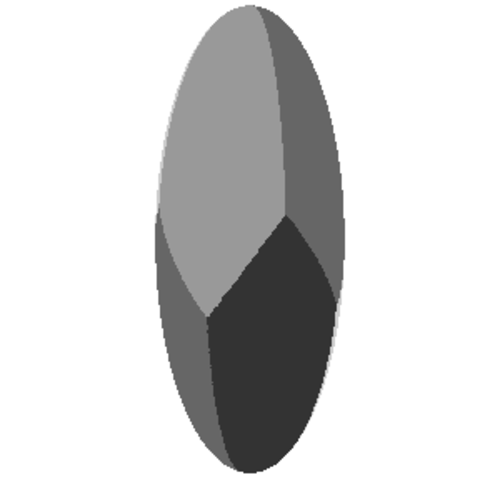
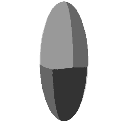
24 Other Parameterization
We have shown that the Euclidean Voronoi diagram and the divergence Voronoi diagram are different as far as the regular parameterization of a quantum state is used. However, the parameterization of the quantum state is not unique. The condition that a matrix is Hermitian and its trace is one is expressed in another way. Here, we show an example of the parameterization with which the section of the diagrams shown in the previous section coincides. Note that it just means the sections are the same and it cannot conclude that the diagrams are globally the same.
It is difficult to investigate all the possible parameterization, or equally all the possible embedding of quantum state space into the Euclidean space. This section is intended only to show an example to which the proof of the previous section cannot be applied.
Suppose that a density matrix is parameterized in another way than Equation (13) as
| (160) |
In other word, we will think what happens if is replaced by . We will show that Voronoi diagrams with respect to Euclidean distance and the divergence coincide for pure states in the section expressed by (133)
Under this parameterization, Equation (144) is expressed as
| (161) |
and Equation (153) becomes
| (162) |
Assuming that Equation (161) holds, the Euclidean distance is calculated as
| (163) |
Therefore,
| (164) |
This is equivalent to Equation (162), and we have shown the Voronoi diagrams are the same.
Again, we mention this does not conclude that the diagrams are the same globally. We conjecture that they are different. More generally, we conjecture that even with any parameterization of quantum state space, the Euclidean Voronoi diagram and the divergence Voronoi diagrams are different.
25 Bures distance and Fubini-Study Distance
In this section, we prove the following theorem:
Theorem 5.6.
In a general level quantum system, for pure states, the following diagrams are equivalent:
- •
diagram with respect to the divergence, i.e.
- •
diagram with respect to Fubini-Study distance
- •
diagram with respect to Bures distance
The equivalence between the Fubini-Study diagram and the Bures diagram is obvious because
Hence we will show the coincidence between the diagram by Bures distance and the diagram by divergence.
For we define
| (166) |
where
| (167) |
In other words, is parameterized by one real parameter and complex parameters . Note that in this parameterization, there might be more than one representations for one given density matrix.
This converges to a pure state when you take the limit . Moreover has rank if , and all pure states in space of level system can be expressed by the limit of . Actually, taking the limit, we obtain
| (168) |
and any pure state can be written in this way.
About the divergence, we will calculate the boundary of the Voronoi diagram as a set of ’s for a fixed , and take its limits. Considering the equivalence of the equations stated in (25), we can restate the problem:
Claim 5.1.
For given pure states and , let
| (169) |
and
| (170) |
Then, for any the following equation holds:
| (171) |
Proof.
Suppose that ’s are expressed as
| (172) |
Defining the matrix by
| (173) |
we can also express
| (174) |
Now we obtain
| (175) |
Denoting by , (175) can be expanded further as
| (176) | ||||
| ( “?” stands for a non-zero element that does not | ||||
| affect the result of the calculation) | ||||
| (177) |
Here note that for because the elements are all zero except the first two columns. Thus, we get
| (178) |
Here we used the fact that
| (179) |
because is unitary and vectors and have a unit length. For Equation (178) to hold independent of , the necessary and sufficient condition is
| (180) |
Writing down the elements by ’s and ’s, we obtain the condition written as
| (181) |
Now we consider the condition for Bures (or Fubini-Study) distance. Similarly we can extend the formula as follows:
| (182) |
Thus,
| (183) |
and finally we obtain the same condition as (181). ∎
26 Expected applications
Although the Euclidean distance is an exception and the space is restricted to pure states, we have shown that the coincidence of the Voronoi diagrams also happens in three or higher system. This means some problem about a distance for pure states can be translated into another problem in another distance. In such a sense, we can say we have clarified the structure of pure states as a space.
As is explained in Section 19, effectiveness of the algorithm by Hayashi et al. to compute the Holevo capacity of one-qubit channel is partially supported by the coincidence of Voronoi diagrams. It is natural to think the extended coincidence for higher level system might become useful in the extended algorithm. The extended algorithm is introduced in Chapter 6, but we have not found a concrete application in it. We also have to mention that the main part of the theorem about the coincidence used to support the effectiveness of the algorithm for one-qubit system is the one between Euclidean Voronoi and the divergence Voronoi, and it is proved not to happen in a higher level system.
The distances in a quantum state space are originally considered as a tool to distinguish the states by measuring. We expect our result will be used in the identification of states. Actually, how well a message is coded in quantum system partially depends on how uniformly distributed points we can get in a quantum state space. The uniformness of a point set is preserved between multiple pseudo-distances if their Voronoi diagrams are the same.
As a real vector space, a -level quantum state space has a quadratic dimension . From the viewpoint of computational geometry, our contribution is an implication about such a large dimensional space about its actual computation. It provides a new category of research fields: distortion measure in a high dimensional space.
27 Summary of this chapter
We have investigated whether the same thing as the coincidence of Voronoi diagrams in the one-qubit system also occurs in three or higher level system. The Euclidean Voronoi diagram and the divergence Voronoi diagram are proved to be different in three or higher level system. On the other hand, for pure states, the coincidence of the Euclidean distance, the Bures distance, and the Fubini-Study distance occurs even in three or higher level system.
Some problems about a pseudo-distance for pure quantum states can be translated into a problem about another pseudo-distance. There is still no concrete application of it, but by the analogy of the numerical computation of capacity of one-qubit channel, it is likely to become useful in the future.
Another point is that we found a connection among measures which have apparently have no relation. Especially, the connection between a distance used for quantum database search and a pseudo-distance used in quantum information theory is meaningful.
Chapter 6 Numerical Computation and Experiment
28 Overview
We propose a new algorithm to compute the Holevo capacity of a quantum channel especially for three or higher level system. Our algorithm is based on a global optimization and never converges to a local optimum. It is the main merit of our algorithm compared to the preceding one.
Osawa and Nagaoka [92] proposed an algorithm to compute the Holevo capacity, which is an extension of the algorithm by Arimoto and Blahut to compute the capacity of a classical channel. The main deficit of the algorithm by Osawa and Nagaoka is that it only computes a local optimum, although Arimoto–Blahut’s algorithm is guaranteed to reach the global optimum. It is because the objective function in the optimization is concave for a classical capacity while it is not concave for a quantum one.
The algorithm we propose is an extension of the one by Hayashi et al. [47] and Oto et al. [93, 94]. We follow their idea of using the smallest enclosing ball problem after approximating the geometric object by a set of points. However, to solve the smallest enclosing ball problem, the method based on a farthest Voronoi diagram explained in [93, 94] cannot be directly applied to a higher level system because of its complexity. Our main contribution is to show theoretically and practically that Welzl’s algorithm to solve the smallest enclosing ball problem is also useful for a quantum state space.
The main merit of our algorithm is that it can find a global optimum although it is only an approximate algorithm. The difference of the ideas between our algorithm and Osawa–Nagaoka’s one is conceptually explained by Fig. 14.


29 Smallest enclosing ball problem in a quantum state space
In this section, we show that Welzl’s algorithm is also applicable for the quantum state space with the quantum divergence as its pseudo-distance.
Matoušek and al. [75] showed that the smallest enclosing problem belongs to the class called linear programming-type (LP-type) problem which is introduced as an abstraction of some algorithm for linear programming. The LP-type problem is defined as follows [75]. Think about the class of the optimization problems defined by pairs , where is a finite set and is a function with a values in a ordered set . The goal is to find the optimal set which satisfies
and for any , .
This problem is LP-type when the following axioms are satisfied.
Axiom 6.1 (Monotonicity).
For any and with , we have
| (184) |
Axiom 6.2.
(Locality) For any with , and any ,
| (185) |
The smallest enclosing ball problem in Euclidean space is obviously belongs to this class. For the smallest enclosing ball problem with respect to a given arbitrary distance in a given space, whether Welzl’s algorithm is also applicable, or in other words, has the same complexity order as in Euclidean space is certified by checking if the axioms above are satisfied.
Nielsen and Nock [80] showed Bregman divergence satisfies the axioms above. We will show that the quantum divergence also satisfies the axioms in the rest of this section, but it is by mostly the same idea of Nielsen and Nock.
The latter axiom, locality, can be proved by showing the uniqueness of the optimal ball. The uniqueness is follows from the linearity of the bisectors (Theorem 5.1).
Note that there are two types of the smallest enclosing ball problem can be considered as
| (186) | |||
| (187) |
where means a given set of quantum states. Our main interest is the second type because it is used to compute the Holevo capacity. The locality can be proved for both. First it is directly proved for the first type. For the second type, we take dual of the problem as in Theorem 5.2, and similarly in the dual space, we can determine the smallest enclosing ball uniquely.
We have shown that for the smallest enclosing ball problem with respect to the quantum divergence, we can reach the optimum following the same process as Welzl’s algorithm. However, note that it is only under the assumption that the most primitive part of the algorithm works. In other words, it can come to no conclusion about the complexity. Actually, it needs a complicated non-linear optimization to find a ball in terms of the divergence which passes through given points. Not only the complexity for it is not known, but there is no guarantee that the solution can be found.
30 Algorithm for numerical computation of the Holevo capacity
For the fixed level of quantum system, the top level procedure of the algorithm we propose is as follows:
Algorithm 6.2.
The function dist_points computes the reasonably distributed points to some extent, qminball computes the smallest enclosing ball with respect to the quantum divergence. As an algorithm for dist_points, we employed the following:
Algorithm 6.3.
The function next_state called from this is as follows. Here, is a constant given as a parameter.
This algorithm is equivalent to run through all the possible tuples of integers which satisfies . The similar mechanism as in a carry-up in the computation of sum of two integer is used in next_state. It tries to add to the -th value , but if the resulting value does not satisfy , is set to and it tries to carry up to the next value .
Since has the same value up to the multiplication of a complex number to (of course, under the condition that because must be a pure quantum state), -th value of vector can be restricted to . So, lines 4 and 5 of dist_points do not lose generality.
We are not convinced that this is the best algorithm for dist_points, but we take a trade-off between the simpleness of the algorithm and the goodness of its distribution. The algorithm is easy to understand, and looks reasonable to generate uniformly distributed points. Nevertheless, there is no theoretical guarantee that it really generates uniformly distributed points.
The main part of our algorithm is the procedure to solve the smallest enclosing ball problem. It is described as follows:
Algorithm 6.4.
The hardest part is the algorithm for b_qmb. b_qmb computes the sphere which passes through all the given points. To implement b_qmb, the non-linear (convex) optimization is necessary, and we have not found the algorithm to compute it certainly. However, we believe that for a small , we can use some general-purpose optimization libraries. We show in the next section that it is a really practical option.
Although there is no 100% reliable way to compute b_qmb, the characteristic of the algorithm that it runs through points globally is a merit to cover that problem. To approximate the final result, it is not necessary to compute the exact value for each call of b_qmb, but it is enough with mostly correct value for mostly all the call of b_qmb. Since it runs through all the plotted points globally, it is enough if the correct value is computed in one of the neighbor of the real optimal point. Of course, here we assume the error is one-sided, i.e. when it returns a wrong ball, the ball is always bigger than the real smallest ball.
The computational error must be considered after divided into two phases. About the smallest enclosing ball problem of points, the error is one-sided. In that phase, the error is because of the optimization process, and if the optimization does not converges to the real optimum, the computed value is always bigger then the real optimum. However, our final objective to compute the Holevo capacity and it is equivalent to solve the smallest enclosing ball of a continuous geometric object. Since a geometric object is approximated by plotting points, one-sidedness of the error is not guaranteed at all.
Of course, we can say we can obtain a better result by plotting more points. Then, how many points are needed to achieve a given upper bound of the error? It is left to be open. It is essential to make the proposed algorithm really practical.
31 Numerical experiment
Now, we show the algorithm we proposed is really practical. We will check whether the samples computed by Osawa and Nagaoka [92] is correct.
The most primitive part to compute the sphere with respect to the divergence which passes through given points (b_qmb in Section 30) is implemented using GNU Scientific Library (GSL) [42]. We used the function gsl_multimin_function_fdf in GSL to compute the minimum value of a given function with its domain in . The optimization problem we have to solve is formulated as follows:
Input: and
Minimize
Subject to
However, GSL has no non-linear optimization function which process the constrains like this. To fit to the specification of gsl_multimin_function_fdf of GSL we rewrite the problem with a sufficiently large number as follows:
Input: and
(188)
Note that the only exception is the case . In that case, the computation of the center of the ball does not include optimization. The center is uniquely determined by equations. Actually, the equation
| (189) |
includes equal marks and unknown variables, and it has a unique solution in general.
We employed a restricted version of the algorithm which ignore the ball with points on its boundary. In other words, we solved the problem under the assumption that the optimal ball is determined by less than points. This restriction is because there is no easy way to compute the solution of Equation (189). Although this restriction seems unnatural, we expect that it makes no difference for the result, or at worst, the difference is small because of the characteristic of the problem.
We compute the capacity for the channel in [92]. is given by
| (190) |
where are given as
| (191) | ||||
| (192) | ||||
| (193) |
The step value ( in Algorithm 6.3) is set to , and the number of plotted points are . This value is determined so that the computation ends in a reasonable time, and returns a reasonable result.
The result of our experiment was , while the optimal value written in [92] is . The arguments to achieve the optimum is shown in Table 2, where the optimal value for is expressed by
| (194) |
and the approximated capacity is given by
| (195) |
The machine used in experiment is Intel Xeon 2.3GHz (64bit) with Linux x86_64 installed. The time for computation was 6 hours and 55 minutes.
Result: 0.6729054
Time for computation: 6h55m
Variables to achieve the optimum:
0.082689
0.15770
0.13717
0.17875
0.21126
0.23243
Fig. 15 shows the result of the computation for various . Since we can approach to the real solution with a smaller , it seems our result is approaching to the result by Osawa and Nagaoka. However, we cannot conclude because we have not estimated the computational error and the error for our algorithm is not one-sided.

32 Discussion
We obtained the similar result as that of Osawa and Nagaoka. Since we have not done any error estimation, we can not know how correct the result is. However, it is still meaningful because we achieved a good approximation for the result of Osawa and Nagaoka, and showed their result is likely to be the global optimum.
In our experiment, the number of quantum states which appears on the surface of the optimum ball is 6, which is bigger than the number 3 shown in the paper by Osawa and Nagaoka. Although it is probably because of an error of the approximation, another possibility is that for the smaller number of points, the optimum is not correctly calculated. Actually we observed that smaller number of points as a constraint makes the optimization more unstable. It is because with fewer constraints, the dimension of the space where the variables can go becomes higher. Anyway, further observation is needed to know the reason for the difference.
To make the approximation better, we have to make the step value smaller. The problem is the computational complexity which rapidly increases as gets smaller. For three level system, when is , the complexity becomes .
To avoid the computationally difficult case, our experiment was under the assumption that the optimum ball is determined by less than points. To remove the restriction is naturally considered as a next work. Although the direct computation of the ball which pass through is to solve a dimensional non-linear equation, the dual problem by Legendre transform becomes a linear equation. Using the dual problem is a probable option.
Another problem is how much likely this method can be used for an arbitrary -level system. For a -level system, the complexity becomes , where . Because of lack of error estimation, we cannot say any concrete criterion for , but it is likely that the computation for is far more difficult than the case .
As is mentioned by Welzl [121], the possible way of improvement is to care for the order of the points. The original algorithm to compute the smallest enclosing ball is a Las Vegas algorithm and its computational complexity is based on the randomness of the order of points. Some heuristics might improve the actual performance of the computation, even if it does not improve the complexity expressed as an order. In particular, since the optimization process for fixed bounding points is very heavy in the proposed algorithm, the heuristics in the order of the points is more likely to contribute to the improvement than the usual Euclidean smallest enclosing ball problem.
33 Summary of this chapter
We proposed a new algorithm to compute the Holevo capacity of a quantum channel which uses arranged version of Welzl’s algorithm to compute the smallest enclosing ball problem. The proposed algorithm is for an arbitrary -level system, and it is natural extension of the existing algorithm for one-qubit system.
Although the proposed algorithm includes a non-linear optimization in its process which is likely to be very unstable, we have shown it is actually works for some examples of channels in 3-level system. We calculated the same examples as the ones by Osawa and Nagaoka [92], and certified the results by them are real optima though there had been a concern that those might be only local optima. The main merit of our algorithm is that it searches an optimum globally.
Although proposed algorithm can practically approximate the result, analysis for its error is not done yet, and the error is not one-sided. Estimating the error and computing the lower-bound for the real value by the computed value are to be done.
Chapter 7 Conclusion
In this dissertation, we have given another geometric interpretation to a quantum state space. It indicates a connection among some quantum-related research fields.
More precisely, what we have shown in this dissertation mainly consists of the following two parts:
- •
some Voronoi diagrams in quantum state space coincides
- •
Welzl’s algorithm for the smallest enclosing ball problem is also applicable for a quantum state space.
In this chapter, we summarize again the main results and discuss the meaning of them and future potential of development of related researches.
34 Coincidences of Voronoi diagrams
We proved that in one-qubit system, the Voronoi diagrams with respect to the divergence and Euclidean distance are the same. We also proved that in an -level system for , that coincidence does not occur.
In three or higher level system, restricting on a certain subspace, we have investigated some distances. We showed that with some unnatural parameterization, Voronoi diagrams with respect to the divergence and Euclidean distance coincide on the supspace. We also showed that Voronoi diagrams with respect to the divergence and the Fubini-Study distance coincide.
The existing only application of these fact is the algorithm by Hayashi et al. [47] to compute the Holevo capacity of a quantum channel. Nevertheless, we believe those result have clarified some aspect of the structure of a quantum state space.
Our result shows thatthere is a connection among different distances which are used in different cotexts. Especially a significant thing is a connection between the distance used in quantum computation and the pseudo-distance which is used for quantum information theory. We regard we indicated a bridge between those research fields.
From the viewpoint of computational geometry, what we have done can be a methodological hint. Generally in a situation that some measures are associated to a set, analyzing those Voronoi diagrams will some indication about the relation of those measures. Especially for a computational purpose, since a Voronoi diagram is a popular tool to approximate a continuous geometric object in a computer, comparing Voronoi diagrams is a reasonable start point for the discussion about how we can deal with a given continuous object with some associated metrics.
35 Numerical computation of Holevo capacity
We have shown that Welzl’s algorithm for the smallest enclosing problem is also applicable to a quantum state space. Using Welzl’s algorithm, we proposed a new algorithm to compute the Holevo capacity of a quantum channel. Although it leads to no conclusion about its complexity, we showed it is practical by an experiment.
Although the experiment is for only few samples and under some restrictions, we showed the proposed algorithm really works for a real computation. We have not compared its practical performance to the existing algorithm by Osawa and Nagaoka [92], but it has at least one merit: there is no worry for local optima.
Since our algorithm is an approximation by plotting points on a continuous geometric object, its performance is trade-off with its error. Consequently, for the future research, the improvement of “uniformness” of plotted points and the error estimation should be considered as a set. The proposed method to generated a “reasonably” uniform points as pure states is only intended to be implemented easily, and no mathematical analysis is given for its uniformness. To improve the algorithm of that part, consideration about what error bound can be attained will be necessary.
Welzl’s algorithm is classified as a Las Vegas algorithm, and its expected time of computation is linear. As is mention by Welzl himself [121], the expected time is based on the randomness of the order of points, but some heuristics about ordering of points might improve the performance. To seek for heuristics specific for a quantum state space is one of the possible extensions of this research.
References
- [1] D. S. Abrams and C. P. Williams. Fast quantum algorithms for numerical integrals and stochastic processes, 1999, http://arxiv.org/abs/quant-ph/9908083.
- [2] R. Alicki and M. Fannes. Note on multiple additivity of minimal renyi entropy output of the werner-holevo channels, 2004, http://arxiv.org/abs/quant-ph/0407033.
- [3] S. Amari and H. Nagaoka. Methods of Information Geometry. AMS & Oxford University Press, 2000.
- [4] G. G. Amosov. Remark on the additivity conjecture for the quantum depolarizing channel, 2004, http://arxiv.org/abs/quant-ph/0408004.
- [5] S. Arimoto. An algorithm for calculating the capacity of an arbitrary discrete memoryless channel. IEEE Trans. Inf. Theory, 18:14–20, 1972.
- [6] T. Asano. Aspect-ratio voronoi diagram and its complexity bounds. Information Processing Letters, 105(1. 31):26–31, 2007.
- [7] T. Asano, N. Katoh, N. Tamaki, and T. Tokuyama. Angular Voronoi diagram with applications. In Proceedings of 3rd International Symposium on Voronoi Diagram in Science and Engineering, pages 32–39, Banff, Canada, 2006.
- [8] T. Asano, N. Katoh, N. Tamaki, and T. Tokuyama. Voronoi diagram with respect to criteria on vision information. In Proceedings of 4th International Symposium on Voronoi Diagram in Science and Engineering, pages 25–32, Wales, UK, 2007.
- [9] D. Avis, J. Hasegawa, J. Kikuchi, and Y. Sasaki. A quantum protocol to win the graph colouring game on all hadamard graphs. IEICE Transactions on Fundamentals of Electronics, E89-A(5):1378–1381, May 2006, http://arxiv.org/abs/quant-ph/0509047.
- [10] D. Avis and T. Ito. Comparison of two bounds of the quantum correlation set. In Proceedings of the 1st International Conference on Quantum, Nano and Micro Technologies (ICQNM 2007), January 2007.
- [11] C. H. Bennet and G. Brassard. Quantum cryptography: Public key distribution and cotin tossing. In Proceedings of IEEE Int. Conf. Computers, Systems and Signal Processing, pages 175–179, Bangalore, India, 1984.
- [12] C. H. Bennett, D. P. DiVincenzo, J. A. Smolin, and W. K. Wootters. Mixed-state entanglement and quantum error correction. Phys. Rev. A, 54(5):3824–3851, Nov 1996.
- [13] E. Biham, O. Biham, D. Biron, M. Grassl, and D. A. Lidar. Grover’s quantum search algorithm for an arbitrary initial amplitude distribution. Phys. Rev. A, 60(4):2742–2745, 1999.
- [14] R. Blahut. Computation of channel capacity and rate distortion functions. IEEE Trans. Inf. Theory, 18:460–473, 1972.
- [15] C. Buckley. A divide-and-conquer algorithm for computing 4-dimensional convex hulls. In Lecture Note in Computer Science, volume 333, pages 113–135. Berlin: Springer-Verlag, 1988.
- [16] D. Bures. An extension of Kakutani’s theorem on infinite product measures to the tensor product of semifinite -algebras. Trans. Amer. Math. Soc., 135:199–212, 1969.
- [17] C. Burnikel, K. Melhorn, and S. Schirra. How to compute the Voronoi diagram of line segments: theoretical and experimental results. In Lecture Note in Computer Science, volume 855, pages 227–239. Springer-Verlag, 1994.
- [18] M. S. Byrd and N. Khaneja. Characterization of the positivity of the density matrix in terms of the coherence vector representation. Phys. Rev. A, 68(062322), 2003.
- [19] CGAL open source project. http://www.cgal.org/.
- [20] K. L. Clarkson and P. W. Shor. Applications of random sampling in computational geometry, ii. Discrete and Computational Geometry, 4:387–421, 1989.
- [21] R. Cleve, A. Ekert, C. Macchiavello, and M. Mosca. Quantum algorithms revisited. Proc. Roy. Soc. London A, page 454(1969):553, 1998.
- [22] N. Datta, A. S. Holevo, and Y. Suhov. Additivity for transpose depolarizing channels, 2004, http://arxiv.org/abs/quant-ph/0412034.
- [23] N. Datta, A. S. Holevo, and Y. Suhov. A quantum channel with additive minimum output entropy, 2004, http://arxiv.org/abs/quant-ph/0403072.
- [24] N. Datta and M. B. Ruskai. Maximal output purity and capacity for asymmetric unital qudit channels, 2005, http://arxiv.org/abs/quant-ph/0505048.
- [25] X. Deng and B. Zhu. A randomized algorithm for Voronoi diagram of line segments on coarse grained multiprocessors. In Proceedings of the 10th International Parallel Processing Symposium (IPPS ’96), pages 192–198, 1996.
- [26] D. Deutsch. Quantum theory, the Church-Turing principle and the universal quantum computer. Proc. Roy. Soc. London A, page 400:97, 1985.
- [27] D. Deutsch and R. Jozsa. Rapid solution of problems by quantum computation. Proc. Roy. Soc. London A, page 439:553, 1992.
- [28] R. L. Drysdale. Generalized Voronoi diagrams and Geometric Searching. PhD thesis, Department of Computer Science, Starnford Universisy, 1979.
- [29] R. L. Drysdale and D.-T. Lee. Generalized Voronoi diagram in the plane. In Proceedings of the 16th Annual Allerton Conference on Communications, Control and Computing, pages 833–842, 1978.
- [30] H. Edelsbrunner. Algorithms in Combinatorial Geometry. Berlin: Springer-Verlag, 1987.
- [31] A. Einstein, B. Podolsky, and N. Rosen. Can quantum-mechanical description of physical reality be considered complete? Phys. Rev., 47(10):777–780, May 1935.
- [32] M. Fannes, B. Haegeman, M. Mosonyi, and D. Vanpeteghem. Maximal output purity and capacity for asymmetric unital qudit channels, 2005, http://arxiv.org/abs/quant-ph/0505048.
- [33] R. Feynman. Simulating physics with computers. Int. J. Theor. Phys., 21:467–488, 1982.
- [34] K. Fischer and B. Gärtner. The smallest enclosing ball of balls: combinatorial structure and algorithms. International Journal of Computational Geometry & Application, 14(4-5):341–378, 2004.
- [35] S. Fortune. A sweepline algorithm for Voronoi diagrams. In Proceedings of the 2nd Annual ACM Symposium on Computational Geometry, pages 313–322, Yorktown Heights, June 1986.
- [36] L. Fritzsche, H. Hellwig, S. Hiller, and O. Deussen. Interactive design of authentic looking mosaics using Voronoi structures. In Proceedings of 2nd International Symposium on Voronoi Diagrams in Science and Engineering, pages 82–92, Seoul, Korea, 2005.
- [37] A. Fujiwara and T. Hashizumé. Additivity of the capacity of depolarizing channels. Phys. Lett. A, 299:469–475, 2002.
- [38] M. T. Goodrich, C. O’Dunlaing, and C. K. Yap. Constructiong the Voronoi diagram of a set of line segments in parallel. Algorithmica, 9(2):128–141, 1993.
- [39] L. K. Grover. A fast quantum mechanical algorithm for database search. In 28th Annual ACM Symp. On the Theory of Computing, pages 212–219. ACM Press New York, 1996, http://arxiv.org/abs/quant-ph/9605043.
- [40] L. K. Grover. A frame work for fast quantum mechanical algorithms. In 30th Annual ACM Symp. On the Theory of Computing, pages 53–62. ACM Press New York, 1998, http://arxiv.org/abs/quant-ph/9711043.
- [41] L. K. Grover. Quantum computers can search rapidly by using almost any transformation. Phys. Rev. Lett., 80(19):4329–4332, 1998.
- [42] GNU Scientific Library (GSL). http://www.gnu.org/software/gsl/.
- [43] D. Halperin and M. Sharir. New bounds for lower envelopes in three dimensions, with applications to visibility in terrains. In SCG ’93: Proceedings of the Ninth Annual Symposium on Computational Geometry, pages 11–18, New York, NY, USA, 1993. ACM.
- [44] D. Halperin and M. Sharir. Almost tight upper bounds for the single cell and zone problems in three dimensions. In SCG ’94: Proceedings of the Tenth Annual Symposium on Computational Geometry, pages 11–20, New York, NY, USA, 1994. ACM.
- [45] M. Hayashi. Asymptotic estimation theory for a finite-dimensional pure state model. Journal of Physics A: Mathematical and General, 31:4633–4655, 1998.
- [46] M. Hayashi. Quantum Information: An Introduction. Springer-Verlag, 2006.
- [47] M. Hayashi, H. Imai, K. Matsumoto, M. B. Ruskai, and T. Shimono. Qubit channels which require four inputs to achieve capacity: Implications for additivity conjectures. QUANTUM INF.COMPUT., 5:13, 2005, http://arxiv.org/abs/quant-ph/0403176.
- [48] S. Heinrich. From Monte Carlo to quantum computation, http://arxiv.org/abs/quant-ph/0112152.
- [49] S. Heinrich. Quantum integration in Sobolev classes. Journal of Complexity, 19:19–42, 2003.
- [50] S. Heinrich. Numerical analysis on a quantum computer. In Lecture Notes in Computer Science, number 3743, pages 28–39. Springer-Verlag, 2006.
- [51] F. Hiai and D. Petz. The proper formula for relative entropy and its asymptotics in quantum probability. Communications in Mathematical Physics, 143(1):99–114, 1991.
- [52] A. Holevo. Bounds for the quantity of information transmitted by a quantum communication channel. Problemly Peredachi Informatsii, 9(3):3–11, 1973. English Translation: Probl. Inform. Transm., 9, 177–183 1975.
- [53] A. Holevo. On the capacity of quantum communicaion channel. Problemly Perecdochi Informatsii, 15(4):3–11, 1979. English translation: Probl. Inform. Transm., 15, 247–253, 1973.
- [54] A. S. Holevo. The capacity of quantum channel with general signal states. IEEE Trans. Inf. Theory, 44(1):269–273, 1998.
- [55] Icking and Ha. A tight bound for the complexity of voronoi diagrams under polyhedral convex distance functions in 3D. In STOC: ACM Symposium on Theory of Computing (STOC), 2001.
- [56] id Quantique SA. http://www.idquantique.com/.
- [57] H. Imai, M. Iri, and K. Murota. Voronoi diagram in the Laguerre geometry and its applications. SIAM Journal of Computing, 14(1):95–105, 1985.
- [58] M. Isenburg, Y. Liu, J. Shewchuk, and J. Snoeyink. Streaming computation of delaunay triangulations. In SIGGRAPH ’06: ACM SIGGRAPH 2006 Papers, pages 1049–1056, New York, NY, USA, 2006. ACM.
- [59] T. Ito. Bell inequalities and the cut polytope: bridging quantum information science and combinatorial optimization. PhD thesis, Department of Computer Science, University of Tokyo, 2007.
- [60] K. Kato, M. Oto, H. Imai, and K. Imai. Voronoi diagrams for pure 1-qubit quantum states. In Proceedings of International Symposium on Voronoi Diagram, pages 293–299, Seoul, Korea, 2005. http://arxiv.org/abs/quant-ph/0604101.
- [61] K. Kato, M. Oto, H. Imai, and K. Imai. On a geometric structure of pure multi-qubit quantum states and its applicability to a numerical computation. In Proceedings of International Symposium on Voronoi Diagram, pages 48–53, Banff, Canada, 2006. http://arxiv.org/abs/quant-ph/0607029.
- [62] K. Kato, M. Oto, H. Imai, and K. Imai. Voronoi diagrams and a numerical estimation of a quantum channel capacity. In 2nd Doctoral Workshop on Mathematical and Engineering Methods in Computer Science (MEMICS 2006), pages 69–76, Mikulov, Czech, Oct. 2006. http://arxiv.org/abs/quant-ph/0611146.
- [63] K. Kato, M. Oto, H. Imai, and K. Imai. Computational geometric analysis of quantum state space and its applications, 2007. Conditionally accepted by Studies on Computational Intelligence, Springer-Verlag (to be published in 2008).
- [64] D.-S. Kim, D. Kim, and K. Sugihara. Voronoi diagram of a circle set from voronoi diagram of a point set, I, topology. Computer Aided Geometric Design, 18:541–562, 2001.
- [65] D.-S. Kim, D. Kim, and K. Sugihara. Voronoi diagram of a circle set from voronoi diagram of a point set, II, geometry. Computer Aided Geometric Design, 18:563–585, 2001.
- [66] G. Kimura. The Bloch vector for -level systems. Physics Letter A, 314(339), 2003.
- [67] C. King. Additivity for unital qubit channles. J. Math. Phys., 43:4641–4653, 2002.
- [68] C. King. Maximal p-norms of entanglement breaking channels, 2002, http://arxiv.org/abs/quant-ph/0212057.
- [69] C. King. The capacity of the quantum depolarizing channel. IEEE Trans. Inf. Theory, 49:221–229, 2003.
- [70] C. King. An application of a matrix inequality in quantum information theory, 2004, http://arxiv.org/abs/quant-ph/0412046.
- [71] C. King and M. B. Ruskai. Comments on multiplicativity of maximal -norms when , 2004, http://arxiv.org/abs/quant-ph/0401026.
- [72] D. G. Kirkpatrick. Efficient computation of continuous skeleskeltons. In Proceedings of the 20th Annual IEEE Symposium on Foundation of Computer Science, pages 18–27, 1979.
- [73] D. Lee and R. L. Drysdale, III. Generalization of Voronoi diagrams in the plane. SIAM Journal of Computing, 10:73–87, 1981.
- [74] MagiQ Technologies, Inc. http://www.magiqtech.com/.
- [75] J. Matoušek, M. Sharir, and E. Welzl. A subexponential bound for linear programming. Algorithmica, 16(4):498–516, 1996.
- [76] K. Matsumoto and F. Yura. Entanglement cost of antisymmetric states and additivity of capacity of some quantum channels. Journal of Phys. A, 37:L167–L171, 2004.
- [77] N. Megiddo. Linear programming in linear time when the dimesion is fixed. J. ACM, 31(1):114–127, 1984.
- [78] A. Miyake and M. Wadati. Geometric strategy for the optimal quantum search. Phys. Rev. A, 64(042717), 2001.
- [79] H. Muta and K. Kato. Degeneracy of angular Voronoi diagram. In Proceedings of 4th International Symposium on Voronoi Diagram in Science and Engineering, pages 288–293, Wales, UK, 2007.
- [80] F. Nielsen, J.-D. Boissonnat, and R. Nock. On Bregman Voronoi diagrams. In ACM-SIAM Symposium on Discrete Algorithms, pages 746–755, 2007.
- [81] F. Nielsen and R. Nock. On the smallest enclosing information disk. Infomation Processing Letters, 2007, doi:10.1016/j.ipl.2007.08.007.
- [82] J. Nishitoba. Smallest enclosing ball orientations of cube graphs. Master’s thesis, Department of Computer Science, University of Tokyko, 2007.
- [83] J. Nishitoba, K. Kato, S. Moriyama, H. Nakayama, and H. Imai. Smallest enclosing balls and an effective calculation of a quantum channel capacity, 2006. submitted to MEMICS 2006.
- [84] E. Novak. Quantum complexity of integration. Journal of Complexity, 17:2–16, 2001.
- [85] T. Ogawa and H. Nagaoka. Strong converse and stein’s lemma in quantum hypothesis testing. Transactions on Information Theory, 46:2428–2433, 2000, http://arxiv.org/abs/quant-ph/9906090.
- [86] M. Ohya, D. Petz, and N. Watanabe. On capacities of quantum channels. Prob. Math. Stats., 17:170–196, 1997.
- [87] A. Okabe, B. Boots, K. Sugihara, and S. N. Chiu. Spatial Tessellations: Concepts and Applications of Voronoi diagrams. Wiley Series in Probability and Statistics. Wiley, 2nd edition edition, 2000.
- [88] K. Onishi. Riemannian Computational Geometry – Convex Hull, Voronoi Diagram and Delaunay-type Triangulation. PhD thesis, University of Tokyo, 1998.
- [89] K. Onishi and H. Imai. Voronoi diagram in statistical parametric space by Kullback-Leibler divergence. In Proceedings of the 13th ACM Symposium on Computational Geometry, pages 463–465, 1997.
- [90] K. Onishi and H. Imai. Voronoi diagrams for and exponential family of probability distributions in information geometry. In Japan-Korea Joint Workshop on Algorithms and Computation, pages 1–8, Fukuoka, 1997.
- [91] K. Onishi and J. Itoh. Estimation of the necessary number of points in riemannian voronoi. In CCCG, pages 19–24, 2003.
- [92] S. Osawa and H. Nagaoka. Numerical experiments on the capacity of quantum channel with entangled input states. IECE Trans. Fund., E84-A(10):2583–2590, 2001.
- [93] M. Oto, H. Imai, and K. Imai. Computational geometry on 1-qubit quantum states. In Proceedings of International Symposeum on Voronoi Diagram, pages 145–151, Tokyo, Japan, 2004.
- [94] M. Oto, H. Imai, K. Imai, and T. Shimono. Computational geometry on 1-qubit states and its application. In ERATO Quantum Information Science (EQIS04), pages 156–157, 2004.
- [95] D. Petz and C. Sudar. Geometries of quantum states. J. Math. Phys., 37(6):2662–2673, 1996.
- [96] F. Preparata and M. Shamos. Computational Geometry: An Introduction. New York: Springer-Verlag, 1985.
- [97] E. M. Rains. Entanglement purification via separable superoperators, 97, http://arxiv.org/abs/quant-ph/9707002.
- [98] S. Rajasekaran and S. Ramaswanmi. Optimal parallel ramdomized algorithms for the Voronoi diagram of line segments in the plane and related problems. In Proceedings of the 10th Annual Symposium on Computational Geometry, pages 57–66, 1994.
- [99] S. Rajasekaran and S. Ramaswanmi. Optimal mesh algorithms for the Voronoi diagram of line segments and motion planning in the plane. Journal of Parallel and Distributed Computing, 26(1):99–115, 1995.
- [100] R. J. Renka. Algorithm 772: Stripack: Delaunay triangulation and Voronoi diagram on the surface of a sphere. ACM Transactions on Mathematical Software, 23(3):416–434, 1997.
- [101] K. Sadakane, H. Imai, K. Onishi, M. Inaba, F. Takeuchi, and K. Imai. Voronoi diagrams by divergences with additive weights. In Symposium on Computational Geometry, pages 403–404, 1998.
- [102] B. Schumacher and M. Westmoreland. Sending classical information via noisy quantum channels. Phys. Rev. A, 56(131), 1997.
- [103] R. Seidel. Constructing higher-dimensional convex hulls at logarithmic cost per face. In Proceedings of the Eighteenth Annual ACM Symposium on Theory of Computing (STOC ’86), pages 404–413, New York, NY, USA, 1986. ACM.
- [104] R. Seidel. Linear programming and convex hulls made easy. In Symposium on Computational Geometry, pages 211–215, 1990.
- [105] C. E. Shannon. A mthematical theory of communication. Bell System Technical Journal, 27:279–423, 623–656, July & October 1948.
- [106] M. Sharir. Intersection and closest-pair problems for a set of planar discs. SIAM Journal on Computing, 14:448–468, 1985.
- [107] M. Sharir. Almost tight upper bounds for lower envelopes in higher dimensions. Discrete and Computational Geometry, 12(1):327–346, December 1994.
- [108] P. Shor. Additivity of the classical capacity of entanglement-breaking quantum channels. J. Math. Phys., 246(3):453–472, 2004, http://arxiv.org/abs/quant-ph/0305035.
- [109] P. Shor. Equivalence of additivity questions in quantum information theory. Commu. Math. Phys., 246(3):473, 2004.
- [110] P. W. Shor. Algorithms for quantum computation: Discreate logarithms and factoring. In 35th Annual Symposeum on Foundations of Computer Science. IEEE Computer Society Press, 1998, http://arxiv.org/abs/quant-ph/9508027.
- [111] K. Sugihara. Artistic pattern generation by a model of territory competing. In Proceedings of 4th International Symposium on Voronoi Diagrams in Science and Engineering, Wales, UK, 2007.
- [112] K. Sugihara and M. Iri. Construction of the Voronoi diagram for “one million” generators in single-precision arithmetic. In Proceedings of the IEEE, volume 80, pages 1477–1484, 1992.
- [113] K. Sugihara and M. Iri. A robust topology-oriented incremental algorithm for Voronoi diagrams. In International Journal of Computational Geometry and Applications, volume 4, pages 179–228, 1994.
- [114] A. Tajima, A. Tanaka, W. Maeda, S. Takahashi, and A. Tomita. Practical quantum cryptosystem for metro area applications. IEEE Journal of Selected Topics in Quantum Electronics, 13(4):1031–1038, July/August 2007.
- [115] B. S. Tsirelson. Quantum generalizations of Bell’s inequality. Phys. Lett. A, 4(2):93–100, 1980.
- [116] B. S. Tsirelson. Quantum analogues of the Bell inequilities: The case of two spacially separated domains. Journal of Soviet Mathematics, 36:557–570, 1987.
- [117] B. S. Tsirelson. Some results and problems quantum Bell-type inequilities. Hanodoroc Journal Supplement, 8(4):329–345, 1993.
- [118] V. Vedral and M. B. Plenio. Entanglement measures and purification procedures. Phys. Rev. A, 57(3):1619–1633, Mar 1998.
- [119] V. Vedral, M. B. Plenio, K. Jacobs, and P. L. Knight. Statistical inference, distinguishability of quantum states, and quantum entanglement. Phys. Rev. A, 56(6):4452–4455, Dec 1997.
- [120] V. Vedral, M. B. Plenio, M. A. Rippin, and P. L. Knight. Quantifying entanglement. Phys. Rev. Lett., 78(12):2275–2279, Mar 1997.
- [121] E. Welzl. Smallest enclosing disks (balls and ellipsoids). In H. Maurer, editor, New Results and New Trends in Computer Science, number 555 in Lecture Notes in Computer Science, pages 359–370, 1991.
- [122] R. F. Werner and A. S. Holevo. Counterexample to an additivity conjecture for output purity of quantum channels, 2002, http://arxiv.org/abs/quant-ph/0203003.
- [123] M. M. Wolf and J. Eisert. Classical information capacity of a class of quantum channels. New Journal of Physics, 7(93), 2005.
- [124] C. K. Yap. An algorithm for the Voronoi diagram of a set of simple curve segments. Discrete and Computational Geometry, 2:365–393, 1987.