Acceleration, Energy Loss and Screening in Strongly-Coupled Gauge Theories
Abstract
We explore various aspects of the motion of heavy quarks in strongly-coupled gauge theories, employing the AdS/CFT correspondence. Building on earlier work by Mikhailov, we study the dispersion relation and energy loss of an accelerating finite-mass quark in super-Yang-Mills, both in vacuum and in the presence of a thermal plasma. In the former case, we notice that the application of an external force modifies the dispersion relation. In the latter case, we find in particular that when a static heavy quark is accelerated by an external force, its rate of energy loss is initially insensitive to the plasma, and there is a delay before this rate approaches the value derived previously from the analysis of stationary or late-time configurations.
Following up on work by Herzog et al., we also consider the evolution of a quark and antiquark as they separate from one another after formation, learning how the AdS/CFT setup distinguishes between the singlet and adjoint configurations, and locating the transition to the stage where the deceleration of each particle is properly accounted for by a constant friction coefficient. Additionally, we examine the way in which the energy of a quark-antiquark pair moving jointly through the plasma scales with the quark mass. We find that the velocity-dependence of the screening length is drastically modified in the ultra-relativistic region, and is comparable with that of the transition distance mentioned above.
1 Introduction and Summary
1.1 Brief overview of earlier work
In the last couple of years, an intense research effort has been directed toward the use of the AdS/CFT correspondence [1, 2, 3] to study parton energy loss in strongly-coupled thermal plasmas. This endeavor is motivated mostly by the quest to understand the quark-gluon plasma (QGP) [4] produced at RHIC [5] and LHC [6], and was stimulated by the pioneering works [7, 8, 9, 10], which were in turn encouraged by the success of the earlier viscosity calculations [11, 12].11 1 Recently it has been argued [13] that, at least at weak coupling, there in fact exists a direct link between viscosity and jet quenching. The phenomenological literature on energy loss is enormous; for reviews, see, e.g., [14, 15].
The drag force experienced by a heavy quark traversing an super-Yang-Mills (SYM) plasma was determined in [7, 8], via its dual description as a string moving on an AdS-Schwarzschild background. The closely related diffusion coefficient was obtained independently in [9]. These seminal papers have been generalized and elaborated on in a vast number of posterior contributions [16, 17, 18, 19, 20, 21, 22, 23], including in particular comparisons with the corresponding weakly-coupled results [24], as well as extensive analyses of the energy-momentum tensor which paint a detailed and beautiful picture of the directionality of energy flow away from the moving quark [25].
A second line of development originated from the work [10], whose authors proposed a recipe for the jet-quenching parameter used in some phenomenological models of energy loss [14], and employed it in the context of SYM. Their calculation has been extended in a number of directions in [26, 17, 27], but also questioned in various ways in [28, 18, 19, 29, 20, 30].
A third line was initiated in [32, 28], which studied mesons moving through an SYM plasma and obtained the corresponding quark-antiquark potential and screening length, using the dual portrayal in terms of a string that moves on an AdS-Schwarzschild background and has both of its endpoints on the boundary. As was emphasized in [32], the outcome would be expected to have implications for the issue of quarkonium suppression in the QGP. Related results were obtained independently in [31], which determined the spectrum of spinning mesons in the confining chiral gauge theory dual to the Sakai-Sugimoto model [33]. Various interesting extensions and refinements of these calculations have been reported in [34, 35, 36, 37, 38, 21, 39, 22, 40].
A notable feature is that, in contrast with the quark probes considered in [7, 8, 9, 10], and the gluon probes studied in [18, 23], mesons do not feel a drag force as they move through the plasma [31, 32, 28]. This is because they are color-neutral, and therefore incapable of setting up the long-range gluonic field profiles that could transport energy away from them.22 2 The color field profile set up by a meson has been explicitly determined at zero temperature in [41, 42]. Indeed, in [18, 22] it has been shown that the other obvious color-neutral probe, the baryon, likewise experiences no drag.
1.2 Motivation and main results
Naturally, the initial papers [7, 8, 9, 10, 32, 28] carried out their calculations under a number of simplifying assumptions. First and foremost among these is of course the use of an SYM plasma as a toy model for the real-world QGP. A number of extensions to other theories that are in certain ways closer to QCD have already been cited above, and a few others can be found in [47]. The issue of how best to compare the SYM and QCD parameters was discussed in [48]. Also important is the restriction to an infinite static plasma. Efforts to examine the case where the plasma is expanding and/or has a finite spatial extent have been made in [49].
The plasma produced at RHIC or LHC has in addition a finite temporal extent, so another issue that could be significant is the limitation of the energy loss computations [7, 8, 9, 10] to the stationary or late-time regime. The actual drag coefficient might be expected to differ from the value obtained in these works in a situation where the quark moving through the plasma is accelerating, or in the initial period following its production within the thermal medium. This point has been emphasized from the phenomenological perspective (in the context of collisional energy loss) in [50], where it was argued that, after a quark-antiquark pair is produced, there exists a significant delay before the rate of energy dissipation coincides with the result relevant for the stationary case. Later works [51] have called into question the actual duration, but not the existence, of this retardation effect.
The estimates in [50, 51] are based on perturbative calculations, so it is interesting to inquire into this effect in the strongly-coupled systems available to us through the AdS/CFT correspondence. It was this question that got us started on the investigation that led to the present work, which over time has expanded toward various other fronts. For simplicity, we have carried out our calculations in the context of an plasma, but we expect most of our qualitative conclusions to apply more generally.
Now, of course, the restriction in [7, 8] to the stationary and asymptotic cases was not made gratuitously, but was necessary in order to gain analytic control on the problem of energy loss. Away from these regimes, the evolution of the quark in the thermal plasma, or equivalently, of the string on the AdS-Schwarzschild geometry, is complicated, and one must resort to a numerical analysis (aspects of which were explored already in [7]). As we will examine closely in due course, the interpretation of the outcome of such an analysis is encumbered by several difficulties, chief among which is our ignorance of the thermal dispersion relation for the quark.
In Section 2 we will gain some perspective on these issues by turning off the temperature , and analyzing first the evolution of an isolated quark in vacuum, which is of interest in its own right, and easier to interpret because in this context the form of the dispersion relation is fixed by Lorentz invariance. We begin in Section 2.1 by reviewing a remarkable paper by Mikhailov [52], who constructed an analytic embedding for the string dual to an infinitely-massive quark in SYM that follows an arbitrary timelike trajectory, and extracted from it a rate of energy loss, Eq. (9), which turned out to agree with the Lienard formula from classical electrodynamics! In the derivation of his result, Mihailov disregarded a total derivative, which we show in (10) to give precisely the expected dispersion relation for the quark. From the results of [52], then, we are able to draw two important lessons: first, that, at any given time, the energy of the string includes not only the portion intrinsic to the quark, but also the part that has been radiated by the quark throughout its previous history; second, that the quark’s dispersion relation arises from a total derivative that ends up being evaluated at the string endpoint.
It is natural to wonder how Mikhailov’s results generalize to the case where the quark has a finite mass, which requires the introduction of probe D7-branes on which the string can end [53]. We examine this issue (still at ) in Section 2.2. Interestingly, we discover that the resulting quark dispersion relation, Eq. (19), as well as the rate of energy loss, Eq. (18), depend on the external force exerted on the quark, or equivalently, on the string embedding parameter , which in the gauge theory controls the shape of the ‘gluon cloud’ surrounding the quark. The dependence is such that the energy and momentum of the quark reduce to the familiar expressions when , and on the other hand diverge as the force approaches its critical value (i.e., the value beyond which would be strong enough to nucleate quark-antiquark pairs out of the vacuum). We finalize our zero-temperature analysis in Section 2.3, noting that the process of energy loss is accompanied by the formation of an event horizon (and a stationary limit curve) on the string worldsheet, as depicted in Fig. 1.
Armed with the intuition afforded to us by Mikhailov’s construction, we proceed in Section 3 to the finite-temperature case. In this setting, we are of course limited by the fact that the general solution to the string equation of motion is not known analytically. Nonetheless, we argue that Mikhailov’s method should admit a generalization, and are able to show in Section 3.1 that this is indeed true for the only thermal solution that is thus far available in closed form, which corresponds to the stationary quark configuration studied in [7, 8]. The resulting dispersion relation, seen in the second and third line of Eq. (34), contains a novel feature that we argue to apply for all finite-temperature configurations, including the quark at rest, Eq. (38): it receives a contribution not only from the string endpoint located on the D7-branes, which is directly dual to the quark, but also from the endpoint located at the black hole horizon, which, as we explain, encodes the initial conditions for the joint quark plasma system.
In Section 3.2 we consider the more general case where the quark accelerates within the plasma. After reviewing the work done in this context by the authors of [7], we pick up precisely where they left off, integrating the string equation of motion numerically for an initially static quark that is accelerated by an external force over a finite period of time and is thereafter released. As shown in Figs. 2,3,4, we find that under such conditions, and for values of the mass in the neighborhood of the charm quark, there exists a period after release where the quark dissipates energy at a rate that is substantially smaller than the stationary/asymptotic result (37) obtained in [7, 8]. Additionally, as seen in Fig. 6, the rate of energy loss in the initial stage where the quark is pushed by the external force can be almost completely accounted for by the generalized Lienard formula (18), describing radiation in vacuum. In (52) and the paragraphs immediately following, we discuss the form of the thermal dispersion relation for the quark subject to the above initial conditions, incorporating the -dependence expected from our zero-temperature results, and explaining in detail the relation to the relativistic expression (46) proposed in [7]. In Section 3.3 we then carry over the discussion of the worldsheet black hole from Section 2.3 to the context, obtaining a time-dependent analog of the Schwarzschild black hole encountered for the stationary case in [19, 20], as schematized in Fig. 7.
Having explored in some depth the effect of the acceleration on the rate of energy loss for an isolated quark, in Section 4 we introduce the other element of realism whose importance was highlighted by the phenomenological studies [50, 51], and examine a quark that is produced together with its corresponding antiquark at some finite time within the thermal medium. The gravity description of this system involves a string with both of its endpoints on the D7-branes, at initially coincident positions. As we review in Section 4.1, an initial exploration of this type of configuration was carried out in [7]. In Section 4.2 we show how the one-parameter family of initial conditions considered in that work can be generalized to describe situations with vastly different patterns of excitations for the initial gluonic fields, and more importantly, to the case where the newly-formed quark and antiquark transform in the adjoint instead of the singlet representation of the color gauge group. Curiously, we find that it is only in the adjoint case that the initial quark velocity is freely adjustable. For the singlet case, as in [7] one must necessarily have , where is the velocity (68) that appeared in different manifestations in the works [31, 32, 28, 19, 20], and on the string theory side of the duality corresponds to the proper velocity of light at the location of the string endpoint [35]. This identification strongly suggests that should be a limiting velocity, as is implicit in at least [35, 19, 20], and is discussed more explicitly in Section 4.3 (as well as in the very recent works [39, 30], which appeared while this paper was in preparation).
In Section 4.4 we study the transition of the - pair to the asymptotic regime described by a constant friction coefficient, which as shown in Fig. 10 applies uniformly to all different types of initial conditions. For singlet configurations, the initial evolution of the quark is of course drastically affected by the presence of the antiquark. In Fig. 11 we determine the velocity dependence of the transition distance beyond which the quark is effectively in the asymptotic regime. For adjoint configurations, on the other hand, the interactions between the quark and antiquark are suppressed at large , and so the two members of the pair evolve independently from the start. In this case we find that the transition distance is essentially zero.
A natural question is whether the transition to the asymptotic regime occurs right after the quark and antiquark are screened from one other by the plasma. This requires a determination of the corresponding quark-antiquark potential, and more specifically the screening length, a problem that we turn to in Section 5. After reviewing and comparing in Section 5.1 the results obtained for infinitely-massive quarks in [32, 28], we generalize to the case of finite mass, first at zero temperature in Section 5.2, and then at finite temperature in Section 5.3. The resulting potentials are shown in Figs. 13, 14. As expressed in (84), (88), (94), they are found to be linear instead of divergent when the quark and antiquark approach one another, signaling the fact that the color sources in this case are no longer pointlike.
In the finite temperature case, the potential implies the velocity-dependence of the screening length presented in Figs. 15,16. As seen there, compared to the infinitely-massive case examined in [32, 28], there is a drastic modification of the behavior at high velocities, which are now bounded by instead of 1. The -dependence near this limit can be determined analytically and takes the form (97), instead of the formula (80) obtained in [32]. Over the whole range , and for masses similar to the charm quark, the behavior can be relatively well approximated by (95), which is the obvious generalization of the fit (78) proposed in [28].
We end the paper by comparing in Section 5.4 the screening length against the transition distance determined in 4.4. For singlet configurations, we find that the magnitude and velocity-dependence of these two separations are comparable, as shown in Fig. 17. Notice that this is in spite of the fact that the two relevant string configurations are rather different. A similar statement can be made for adjoint configurations, where both the screening and transition lengths are essentially zero. We conclude then that, for - pairs created within the plasma, the transition to the asymptotic, constant-drag-coefficient regime takes place immediately after the quark and antiquark lose contact with one another. That is to say, there is no intermediate stage where the quark and antiquark decelerate independently from one another at a rate that differs substantially from the asymptotic result of [7, 8].
Our analysis in Section 3.2 demonstrates that the gluonic fields around a quark can be disturbed by the application of an external force, to the point of producing a significant modification of the energy dissipation rate in the period immediately following release. By analogy with the results we obtained for singlet quark-antiquark configurations in Section 4.4, we interpret this to mean that the quark has to escape far enough from the disturbed region in order to be screened from its effect. In any event, given that the actual experimental situation resembles the setup of Section 4 much more closely than that of Section 3.2, the main overall lesson for QGP phenomenology would appear to be that, beyond an initial period which is controled by the screening length, and where the evolution can be modeled relatively well as taking place in vacuum (and, as such, would be present also in proton-proton collisions), the stationary/asymptotic rate of energy dissipation determined in [7, 8, 9] gives a good approximation to the actual time-dependent dynamics.
It is worth emphasizing that the inferences made in this paper regarding dispersion relations and energy loss rates are based on the natural split achieved in [52] of the total energy of the string. The latter is conserved on the fixed AdS-Schwarzschild background, but would of course decrease steadily if we take into account the gravitational (and dilatonic, etc.) radiation given off by the string in the course of its evolution. Through the GKPW recipe for correlation functions [2], it is this radiation (or, more precisely, the full metric perturbation produced by the string), evaluated at the AdS boundary, that determines the expectation value of the gauge theory energy-momentum tensor. As has been meticulously studied in [25], this tensor contains not just the gross information about the total energy loss rate, but even the fine details about the directionality of the flow and the relative weight of the various dissipation channels. It would therefore be very interesting to examine more closely this link between dissipated energy as encoded on the string and on the gravitational field ultimately generated by it.
2 Single Quark Evolution: Zero Temperature
To analyze the motion of heavy quarks in a strongly-coupled SYM plasma with coupling and temperature , one must follow the evolution of open strings that end on a stack of D7-branes [53] living on the (AdS-Schwarzschild) geometry
| (1) | |||||
where denotes the string length. In our work the string will be taken to lie at a fixed position on the (consistent with the corresponding equations of motion), so the angular components of the metric will not play any role. The D7-branes cover the four gauge theory directions , and extend along the radial AdS direction up from the boundary at to a position where they ‘end’ (meaning that the that they are wrapped on shrinks down to zero size), whose location is related to the quark mass in a way that we will specify below.
From the gauge theory perspective, the introduction of the D7-branes in the background (1) is equivalent to the addition of hypermultiplets in the fundamental representation of the gauge group, breaking the supersymmetry down to . These are the degrees of freedom that we refer to as ‘quarks,’ even though they include both spin and spin fields. For , the backreaction of the D7-branes on the geometry can be sensibly neglected; in the field theory this corresponds to working in a ‘quenched’ approximation which disregards quark loops (as well as the positive beta function they would generate).
The string dynamics follows as usual from the Nambu-Goto action
| (2) |
where () denotes the induced metric on the worldsheet. In the static gauge , , and for motion and deformation of the string purely along direction , the non-zero canonical momentum densities are given by
| (3) | |||||
where of course , . Notice that, due to our normalization of , the must be multiplied by to obtain the physical energy and momentum densities.
In the present section we will restrict attention to the case of vanishing temperature (), in which case we are left in (1) with a pure AdS geometry, and the D7-brane parameter is inversely proportional to the Lagrangian mass of the quark,
| (4) |
A quark that accelerates in vacuum would be expected to emit chromoelectromagnetic radiation. This problem has been examined from the classical perspective in [54], and quantum-mechanically at weak coupling in, e.g., [55]. First steps towards a strong-coupling analysis by means of the AdS/CFT correspondence were taken in [41], which employed tools developed in [56] to study the dilatonic waves given off by small fluctuations on a radial string in AdS5, and infer from them the profile of the gluonic field in the presence of a quark undergoing small oscillations. The results of [41] painted an interesting picture of the propagation of nonlinear waves in SYM, but did not allow a definite identification of waves with the falloff associated with radiation. Very recently, this falloff has been successfully detected in the same setup as [41] through a calculation of the energy-momentum tensor [57], which appeared while this paper was in preparation.
2.1 Infinite mass
The first definite characterization of the radiation rate off an accelerating quark was found much later than [41], and by a completely different route, in an important paper by Mikhailov [52]. Remarkably, this author was able to solve the full nonlinear equation of motion for a string on AdS5, for an arbitrary timelike trajectory of the string endpoint dual to a heavy quark! In terms of the coordinates used in (1) (where for now ), his solution is
| (5) |
with , and the worldline of the string endpoint at the AdS boundary— or, equivalently, the worldline of the dual, infinitely massive, quark— parametrized by the proper time defined through , where . Equation (5) displays the string worldsheet as a ruled surface in AdS5, spanned by the straight lines at constant .
Combining (1) and (5), the induced metric on the worldsheet is found to be
implying in particular that the constant- lines are null, a fact that plays an important role in Mikhailov’s construction. In the solution (5), the behavior at time of the string segment located at radial position is completely determined by the behavior of the string endpoint at a retarded time obtained by projecting back toward the boundary along the null line at fixed . From the component of (5), parametrizing the quark worldline by instead of , and using , where , this amounts to
| (6) |
where the endpoint velocity is meant to be evaluated at . In these same terms, the spatial components of (5) can be formulated as
| (7) |
Working in the static gauge , , the total energy of a string that extends all the way down to the boundary— i.e., with , corresponding to an infinitely massive quark— follows from the Nambu-Goto action (2) as
| (8) |
Using (6) and (7), Mikhailov was able to reexpress this energy (via a change of integration variable ) as a local functional of the quark trajectory,
| (9) |
where of course . The second term in the above equation arises from a total derivative that was not explicitly written down by Mikhailov, but can easily be worked out to be
| (10) |
which gives the expected Lorentz-invariant dispersion relation for the quark. The energy split achieved in (9) therefore admits a clear and pleasant physical interpretation: is the intrinsic energy of the quark at time , and the integral over encodes the accumulated energy lost by the quark over all times prior to . No less remarkable is the fact that the rate of energy loss for the quark in this strongly-coupled non-Abelian theory is found to be in precise agreement with the standard Lienard formula from classical electrodynamics!
2.2 Finite mass
It is interesting to consider how these results are modified in the case , where the mass of the quark given by (4) is large but not infinite. As we have reviewed above, in Mikhailov’s original solution (5) the evolution of the string at any radial position follows from knowledge of the trajectory of the endpoint at the AdS boundary. For a finite-mass quark, we ought to impose boundary conditions on the string not at but at : given the worldline of the quark, we must require that the string worldsheet satisfy . Moreover, we need only determine the behavior of the string in the region .
The required physical solution can of course be viewed as merely the portion of one particular instance of the general solution found by Mikhailov. Our task is therefore to reexpress (5) in terms of the data at the new boundary , instead of the (now merely auxiliary) data at the AdS boundary , which we will henceforth distinguish with a tilde: . For simplicity, we will carry out this translation explicitly only in a setup where the quark moves purely along direction , which is all that we will need for our analysis in subsequent sections.
It follows from (6) and (7) that, at any given point on the string worldsheet,
| (13) | |||||
where denote the velocity and acceleration at the point on the AdS boundary obtained by projecting back from along a null trajectory. From (13) we can deduce that
| (14) |
Evaluated at the new boundary , this formula relates the velocity of the actual string endpoint— i.e., the velocity of the finite-mass quark— to the velocity and acceleration of the ‘auxiliary endpoint’ at . Equation (14) implies that the quark acceleration depends not only on and , but also on the second time derivative of . Because of this, it is not possible to solve for and , the quantities that appear directly in Mikhailov’s energy formula (9), in terms of and , the data that we would naively expect to suffice to characterize the rate of energy loss of the heavy quark.
On the other hand, from (6) and (7) we can infer as well that
| (15) |
so it is certainly possible to solve for in terms of and . Notice that when , we automatically have , which explains why this parameter was not needed in the description of the infinitely-massive quark. For , the value of encodes how much the string tip tilts away from the vertical. But what does this mean in gauge-theoretic language? Through a calculation of or in parallel with that of [56, 41, 25], the slant of the string will have an impact on the shape of the gluonic field profile in the immediate vicinity of the heavy quark: for , this profile is not spherically symmetric. We find it physically more transparent to express the rate of energy loss in terms not of but of the string momentum density given by (3), which by use of (14) and (15) can be rewritten as
| (16) |
When evaluated at , this controls the external force acting on the string endpoint, or equivalently, on the quark.
Inverting (14) and (16), we find
| (17) | |||||
where we have abbreviated . Using this and (13) in (9), we finally conclude that the total energy of the string at time is given by
| (18) |
As before, the first term represents the accumulated energy lost by the quark at all times prior to : it is the generalization to the case of the Lienard formula (9) deduced by Mikhailov. The second term again denotes a surface term and gives the modified dispersion relation for the finite-mass quark,
| (19) |
Notice that , which for and differs from the result expected for a pointlike quark, . This reflects the fact that the fundamental source dual to a string that terminates at is indeed not pointlike. According to the standard UV/IR connection [58], it has a linear size of order , and it is only because of this extended nature that, as we saw above, to characterize its state one needs to specify not only the velocity but also the parameter (or ) that encodes its shape. The crucial point here is that the source in question should not be thought of as a bare quark, but as a ‘dressed’ or ‘constituent’ quark, surrounded by a gluonic cloud with thickness [59, 60]. We will see more evidence of this in Section 5.
Another salient feature of the energy and momentum of the quark given by expressions (19) and (21) is the fact that they both diverge as the value of the external force approaches
| (22) |
The reason for this is easy to understand on the string theory side. To exert a force on the string endpoint, within the D7-branes we must turn on an electric field that has strength at . Working in static gauge, the Born-Infeld Lagrangian on the D7-branes is then
which is real at only as long as the electric field is below the value . Through (4), this is seen to coincide with the value of the critical force (22). The physical origin of this bound is the fact that, for , the creation of open strings is energetically favored, and so the system is unstable. According to (19) and (21), then, the energy and momentum of the constituent quark diverge precisely at the point where the external force becomes capable of nucleating quark-antiquark pairs.
2.3 Late-time behavior and worldsheet black hole
It is interesting to consider the evolution of the string in the case where the quark is accelerated by an external force over some period of time and is then set free at a time . If we put () in (17), then (the acceleration of the auxiliary endpoint of the string vanishes), which in turn implies through (14) and (15) that and at all points on the same null (constant ) line, independently of the value of . In particular, the lower () endpoint of the string travels at speed , which means that that, for , the quark moves at constant velocity , as one would expect given the fact that it is in vacuum.
As time progresses, the null line that departs from the point , which according to (6) is given by
| (23) |
reaches further away from the AdS boundary, so there is an increasing portion of the string () that is completely vertical and moves with the same final velocity . As , this vertical segment describes a quark that moves at constant speed and is surrounded by a stationary gluonic field profile, related to that of a static quark through a Lorentz transformation.
At any given time , then, the energy and momentum previously radiated by the quark are stored as excess energy and momentum on the portion of the string above . This suggests the existence of a geometric region on the worldsheet that ‘absorbs’ the surplus and .
To define this region more precisely, we should note first that, for the spacetime metric (1) (with ), null curves on the worldsheet obey
| (24) |
with the upper or lower sign for the upward- or downward-pointing half of the future light cone, respectively. Using (14), (15) and (17), this translates into
| (25) |
and
| (26) |
where, as before, and refer to the velocity and external force at , evaluated at the retarded time corresponding to the given . As mentioned earlier, Mikhailov’s constant- lines (6)-(7), and (23) in particular, are null, and indeed they can be easily seen to satisfy (25).
If we follow the point as (reaching the spacetime horizon for the Poincaré patch, ), and then project back along the downward pointing light half-cone , we delineate a region () on the string worldsheet from which, by construction, no signal can escape to the asymptotic region corresponding to the final vertical and stationary segment of the string. In other words, the curve so obtained, which we will henceforth denote by , is the event horizon of a worldsheet black hole.
A worldsheet black hole figured prominently in the energy loss analysis of [20, 19], concerning a quark in a thermal plasma. Those works considered the steady-state configuration where the quark moves at a constant velocity ; as a consequence, the black hole they encountered was static, with an event horizon located at the fixed position , precisely the radius that played a crucial role in the drag force calculation of [7, 8].
In our non-stationary system, on the other hand, the worldsheet black hole is dynamical. Let us focus for concreteness on the case where the quark is static up to a time , and is then accelerated until . The location of the event horizon will begin descending from even before (in anticipation of the disturbance produced by the acceleration at the lower endpoint), reach a minimum value of the radial coordinate, and then move up again, approaching as . Notice from (26) that, at any given , the light half-cone can only point towards increasing for sufficiently large (and, for any given , it will point upward for sufficiently large ). This means that the entire upward portion of must lie within the region of maximal disturbance of the worldsheet, i.e., in the diagonal swath between and .
As usual, determining the exact location of the event horizon is difficult due to the global character of its definition: one must know the entire history of the string and then integrate (26), subject to the stated final condition. It is, however, easy to pinpoint with this same equation the location on the worldsheet where , which gives a lower bound on the upward portion of (where, by definition, one has ). From (26), this happens at
| (27) |
where, again, the external force is meant to be evaluated at the retarded time appropriate for the given . At any point along this curve, the downward light half-cone is horizontal (or, equivalently, ), so timelike trajectories must necessarily point towards larger . In other words, is a stationary-limit curve, and the region between it and the upward portion of the event horizon is the analog of an ergosphere, a concept whose relevance has been noted previously in the context in [29]. Setting in (27) implies , so, unlike the event horizon, the stationary limit curve is located fully within the diagonal region between and . It follows from the definitions of the two curves that crosses precisely when the former attains its minimum value, and so the downward portion of the horizon lies below and to the left of . The situation is summarized in Fig. 1.

It is interesting that at the notion of a worldsheet black hole plays as much of a role as in previous analyses at finite temperature. The appearance of such causal structure is seen then to be intrinsically tied to energy dissipation, be it within a thermal plasma or in vacuum. We will examine the former case in Section 3.3. It would be nice to develop this picture further by exploring the relation between the rate at which energy crosses the black hole horizon and the modified Lienard formula in (18).
3 Single Quark Evolution: Finite temperature
Having understood the rate of energy and momentum loss and dispersion relation for a heavy quark that moves in the SYM vacuum, in this section we restore — and consequently — in the metric (1), to study the same quantities in the case where the quark moves through a thermal plasma. In this case, the position where the D7-branes ‘end’ is related to the Lagrangian mass of the quark through [7]
| (28) |
A thorough generalization of Mikhailov’s analytic results [52] to this finite temperature setup would require finding the exact solution to the Nambu-Goto equation of motion for the string on the AdS-Schwarzschild background, for any given trajectory of the string endpoint at . Sadly, we have not been able to accomplish this feat. Nevertheless, based on the results discussed in the previous subsection, we expect the total energy of the string at any given time to again decompose into a surface term that encodes the intrinsic energy of the quark and an integrated local term that reflects the energy lost by the quark.
A priori it might not be obvious that the rate of energy loss in the presence of the strongly-coupled non-Abelian plasma should be given by some expression that depends just on the behavior of the quark at the given instant, and not on its previous history. But in the AdS/CFT context, this property is strongly suggested by the fact that the energy of the string is given by a local expression on the worldsheet just as much in the AdS-Schwarzschild background that is dual to the thermal plasma as in the pure AdS background that corresponds to the SYM vacuum (which, one should not forget, is in itself a nonlinear medium). Starting with written as an integral over , it should again be possible to project back to the boundary along null trajectories, to obtain a formula that depends locally on the quark worldline . The main difference with the zero-temperature case would be that the null trajectories are no longer straight lines.
3.1 Constant velocity
We have verified that these expectations are borne out in the case of the only finite-temperature solution that is known analytically: the stationary configuration of [7, 8],
| (29) |
which describes a quark moving at constant velocity . Any given point on this worldsheet is connected to a point on the AdS boundary by a null curve , defined by
| (30) |
This equation can be integrated to give
| (31) |
in terms of which the stationary solution (29) can be written in the form
| (32) |
Knowledge of this solution allows the total energy of the string,
| (33) |
to be reexpressed as
| (34) |
Similarly, the total momentum of the string,
| (35) |
can be rewritten in the form
| (36) |
As expected, the integrated term in the top line of (34) and (36) recovers the result for the stationary rate of energy and momentum loss obtained in [7, 8],
| (37) |
The terms in the second and third line of (34) and (36), then, codify the energy and momentum that are intrinsic to the quark. We can see that, just like at zero temperature, reduces to only in the pointlike limit .
An important difference with respect to the case analyzed in the previous subsection is that here the surface contribution that determines the quark dispersion relation arises not only from the lower () but also from the upper () endpoint of the string. This is in fact the generic situation in the case, and holds even for the static radial string, where there is of course no energy loss term and is given just by a boundary contribution that defines the thermal rest mass of the quark,
| (38) |
Clearly the second term in (38), just like the terms in the third line of (34) and (36), arises from the string endpoint located at the black hole horizon. It is natural then to wonder to what extent these terms should be regarded as a contribution to the intrinsic energy of the quark, because their value at any given time does not depend on the parameters and (or ) that characterize the state of the lower endpoint at the same instant. In fact, since marks the position of an event horizon, for any finite coordinate time the value of the surface contribution at is not influenced by the behavior of the portion of the string, but depends only on the string’s configuration at . The same interpretation can be then carried over to the gauge theory: the seemingly extraneous terms represent a contribution to the energy of the state that depends solely on the initial configuration of the quarkplasma system. Throughout the evolution, causality guarantees that the behavior of the SYM fields at spatial infinity can only be affected by the initial configuration at , so we can equivalently think of the surface terms at as encoding information on the asymptotic boundary conditions for the system. Indeed, for dynamical processes, the radial location in AdS-Schwarzschild corresponds to the deep IR of the gauge theory.
We conclude then that, to the extent that we wish to compare the energies of configurations with different initial/boundary conditions, it is important to keep track of the terms arising from the surface contribution at the horizon, despite the fact that they are generally independent of the parameters and associated with the intrinsic dynamics of the quark. Notice, in particular, that with this interpretation the negative sign in the second term of (38)— which is at first sight unexpected when viewed as the leading-order thermal correction to the quark mass [19]— becomes easier to digest: it reflects the screening effect of the plasma on the long-range gluonic fields set up by the quark, which implies a reduction of the energy stored in the IR, in comparison with the case.
It is instructive to compare (34) with the alternative split achieved in [7],
| (39) |
with . If one could interpret this latter quantity as the total distance traversed by the quark since the beginning of time, then the first term in (39) would give the overall energy lost by the quark, at the known rate (37), in the total elapsed time . In view of (38), the second term would then imply a standard relativistic dispersion relation for the quark, with mass .
The problem with this interpretation, however (alluded to already in [7]), is that it does not properly address the issue of initial conditions. The actual distance travelled by the quark is by definition , which agrees with only if .33 3 When writing expressions like , we of course have in mind evaluating the corresponding quantities at a time that is fixed but arbitrarily far in the past. This last equality would hold if we had started at with the quark at rest (i.e., with the string static and completely vertical), but the energy-loss term in (39) makes no allowance for an initial period of acceleration.
In contrast with this, the separation obtained in (34) has a clear geometric origin in the context of the generalization pursued here of Mikhailov’s work [52] to the finite-temperature case. Within this framework, the portion of the total string energy that is contributed by the segment of the string in the immediate vicinity of the horizon (located at in the notation of (29), or in the notation of (32)) was lost by the quark at a particular time in the distant past that can be deduced from (31). Since this is the highest segment of the string that contributes to , marks the precise instant when we need to begin our accounting of the energy lost by the quark. At the lower endpoint of the string (and, hence, the quark) was found a distance behind the location of the upper endpoint at , which according to (32) translates into
By this logic, the total energy lost by the quark is given by an expression of the same form as the first term of (39), but with replaced by the actual total distance . And indeed, we see that the integrated term in the first line of (34) is larger than the putative energy loss term in (39) precisely by the amount , and, correspondingly, the intrinsic energy of the quark identified in the second and third line of (34) is smaller by this same amount than what (39) would have indicated.44 4 The fact that, in going from (34) to (39), part of the total derivative has been shifted back to the integrated term might give the impression that the split between the intrinsic energy of the quark and the energy that has already been lost is inherently ambiguous. The wide latitude available in this case, however, stems from the steady-state nature of the configuration under scrutiny. In the general case, clearly it is a very non-trivial property for a particular contribution to the energy of the string to be expressible as a functional only of the state of the endpoints at the given instant.
3.2 Accelerated quark
Having gained some intuition from the analysis of a quark moving as in [7, 8] at constant speed relative to the strongly-coupled plasma, let us now turn our attention to the more general situation where the quark accelerates. In [7], a few important steps were taken to have a better understanding of this case; in the next few paragraphs we will briefly review the key results.
A quark that undergoes any type of (forced or unforced) motion (and, in the former case, is thereafter released) will be slowed down by its interaction with the plasma, and eventually come to rest. The authors of [7] studied the late-time (and consequently low-velocity, low-acceleration) behavior of such a quark, by considering small, exponentially damped fluctuations around the final rest configuration. In dual language, this involves a determination of the quasi-normal modes on the worldsheet of a static and purely radial string. From their analysis they were able to numerically deduce, for any given quark mass parameter , the value of the drag coefficient
| (40) |
As long as one maintains the restriction to the non-relativistic regime, the above definition is equivalent to , and by construction yields a result that is independent of (or ). A few representative values were tabulated in [7].
Additionally, the authors of [7] gave an analytic derivation of the low-velocity dispersion relation for the quark, which they found to take the form
| (41) |
where is the thermal rest mass (38), and
| (42) |
the kinetic mass of the quark. In the heavy quark limit (), where (38) and (28) imply that
| (43) |
they found from their quasi-normal mode calculation that
| (44) |
which through (42) leads to
| (45) |
It was noticed in [7] that expressions (41) and (44), valid in the low-velocity, low-acceleration regime, as well as the value of the drag coefficient (40) deduced from (37), valid for a quark with constant but otherwise arbitrary velocity, are consistent with a relativistic dispersion relation of the form
| (46) |
Additional evidence for this relation was found from the analysis of back-to-back motion of a quark and antiquark formed within the plasma. The results of [7] in this setting will be reviewed and extended in Section 4.
In view of the discrepancy between (46) and the relation that one would naively infer from the second term in (39), the authors of [7] emphasized the need for a more detailed study of the quark’s intrinsic dynamics, and proposed a plan of attack. They observed that if one starts with the quark at rest in the hot medium, and then accelerates it with an external force, then as long as energy dissipation is negligible, it is natural to define the total intrinsic energy of the quark as the initial rest energy plus the work done by the external agent. Motivated by this proposal, we have studied the early-time behavior of a quark initially at rest, which is accelerated by a time-dependent external force that is turned off after a short period of time, allowing the quark to move thereafter only under the influence of the plasma.
As we already mentioned, regrettably, we have not been able to find a general exact solution to the Nambu-Goto equation of motion for the string in the non-stationary case. Nevertheless, it is certainly possible to find numerical solutions that describe string configurations dual to the gauge theory setup described above. Starting at , a string extending from a fixed value of the radial coordinate to the horizon at , initially at rest and vertical, is accelerated by applying an external force to its lower endpoint. After a time , this external force is set to zero and the string moves freely in the curved background.
Using (1) and (2) and imposing the condition that the string moves only in the direction, the equation of motion is
| (47) |
and we must set the initial and boundary conditions to be
| (48) |
The first two conditions here simply implement the requirement that the string start out being static and purely radial. In the third condition, for a given external force acting on the quark, the function could be determined using the relation (3) between and . In practice we find it easier, however, to specify and use the results of the numerical integration together with (3) to deduce the associated . By studying a number of different examples, we have verified that the instantaneous rate of energy loss after the quark is released is independent of our choice of and , i.e., the quark does not care about its past history. For the trajectories that we will plot below, we have used , with and adjustable .
The fourth and final condition in (48) specifies that the string endpoint at the horizon remain fixed, reflecting the fact that the wavefront for the disturbance produced by the external agent at the endpoint of the string will not reach before an infinite amount of (boundary) time has elapsed. In order to implement this condition in our numerical integration, we have set at a radial cutoff , and considered in all cases an integration time smaller than the time that it takes the wavefront to reach the cutoff.
For applications of this formalism to phenomenology, we must choose values of the mass parameter based on the charm and bottom quark masses, GeV. The issue of how best to translate between the SYM and QCD parameters has been discussed in [48]. Taking (), and MeV, and employing the “obvious” prescription and , from (28) we find that for charm and for bottom. If, on the other hand, one uses the “alternative” scheme (motivated in [48] through a rough matching of the AdS/CFT and lattice quark-antiquark potentials) and MeV (which follows from equating the energy densities of the two theories), then (28) leads to for charm and for bottom. In our analysis, we have covered a significant range of masses, but below we will present the results only for three representative values in the neighborhood of the charm mass: .
We have carried out the numerical integration of (47) subject to (48) using the NDSolve routine of Mathematica 5.2. Based on the variation of our results upon doubling the number of integration steps, we estimate our numerics to be accurate to better than . The integration time shown in all plots is given in units of 1/, which (for MeV) corresponds to under the “obvious” and under the “alternative” prescription of [48]. Unfortunately, the numerical integration degrades rather quickly, so in either scheme our investigation is limited to intervals that are an order of magnitude below the experimental timescale of the plasma (typically ). For the same reason, even though the quark can be taken to relativistic velocities at the point of maximal acceleration, we can only achieve rather small velocities at the time of release (for the most part, ).
Our results show a qualitative difference between the initial stage () where the quark is accelerated by means of the external force , and the second stage () where it moves only under the influence of the plasma. We will begin by discussing the latter stage, which would appear to be more relevant from the phenomenological perspective.


The most direct way to inquire whether the output of our numerical integration for the accelerated quark conforms to the the constant-velocity (or late-time) results of [7, 8] is to compare the corresponding quark trajectories. If one assumes the dispersion relation (46), then the equation of motion for a quark subject only to the drag force (40) with constant is
| (49) |
whose solution is [7]
| (50) |
As we already mentioned, in our numerical results , so we are only able to test the non-relativistic version of (50),
| (51) |
(and, since our integration is limited to small time intervals, we would in effect see just the linear portion of this function). A comparison between this analytic prediction and our numerical results for is given in Fig. 2. It is evident from this plot that, in the early stage of motion covered by our analysis, the quark dissipates energy at a rate much lower than the late-time result of [7]. Indeed, for the asymptotic friction coefficient is respectively , but our numeric results for are best approximated by .
We can also attempt to perform the comparison directly at the level of energy loss rates. An important drawback of working with the numerical solution, however, is that we cannot achieve a direct splitting of the total energy of the string, as we did in the stationary case (as well as in the general case at zero temperature). This means that, a priori, we know neither the correct form of the quark dispersion relation nor the formula for the rate of energy loss. But, given that their sum remains constant throughout the evolution, finding a prescription for one of these two quantities would enable us to compute the other.
The authors of [7] assumed that the energy loss would be negligible for sufficiently short acceleration intervals (i.e., for small ), because the drag force exerted by the plasma would not have been able to perform a substantial amount of work. If true, this would allow a direct empirical determination of the dispersion relation. Unfortunately, the situation is not so simple, because, as we learned in Section 2, the quark loses energy through radiation even in the absence of the plasma, and this effect must be taken into account to establish what fraction of the total string energy is intrinsically ascribable to the quark.
To attempt to cut this Gordian knot, we should recall, from our study of the cases where we had analytic control, that the dispersion relation arises as a surface term, with contributions from both endpoints of the string. Based on our previous results, we expect the dispersion relation for the quark in the thermal medium to take the form
| (52) |
The first term here has been copied from the expression (19) (again abbreviating ), and is meant to approximate the contribution from the string endpoint lying on the -branes. The second term arises from the endpoint that reaches the horizon, which we understood above to encode information about the initial conditions. Knowing that our starting configuration is static, we can simply read off this contribution from the second term in the rest energy (38), which we have interpreted as a screening effect. Including this term is important to ensure that (52) reduces to the correct result in the case of a quark that is static and unaccelerated, .
Clearly equation (52) is just an approximation, because the first term should receive thermal corrections. In particular, it is natural to expect the factor of in the denominator to be replaced by , so that, just like in the case, the quark energy diverges at the critical value of the electric field, which now corresponds to [20]. More generally, since the background metric (1) knows that only through the factor , any corrections to the surface term due to the presence of the plasma should be of order or , and are consequently small in the heavy quark regime . For the phenomenologically interesting values , the error in the dispersion relation (52) is estimated to be (much larger than our numerical error).
Notice that (52) without any corrections should give the exact dispersion relation in the infinite-mass limit that has been the focus of many AdS/CFT investigations of energy loss (e.g., [8, 25]). In this limit one is left with
| (53) |
i.e., the -dependence drops out and, just like in the context at the end of Section 2, one recovers pointlike behavior. We can see that, as expected, the first term in (53) agrees with the limit of the second line of the stationary expression (34), but the second term in (53) disagrees with the limit of the third line of (34), due to the different initial conditions.
Expression (52) as a whole looks superficially rather different from the dispersion relation (46) proposed in [7]. In particular, (46) evidently cannot reproduce the - (or -)dependence seen in (52), whose presence is supported by the zero-temperature results of the previous subsection. It is important to remember, however, that such dependence indeed would not have been visible in the quasi-normal mode analysis used to derive (41) or in the quark-antiquark evolution that gave part of the support for (46), because in those calculations the external force was taken to vanish.
Setting , (52) reduces to , while (46) translates (via (38) and (45)) into . The two expressions differ in the form of the second, -independent term, which we have understood to encode the initial conditions for the gauge system. Given that the initial conditions for all situations considered in [7] differ from our current setup, there is no reason why we should expect the corresponding terms to agree. Beyond this, there also appears to be a discrepancy in the order of magnitude for the corrections to the two expressions. We remain puzzled by this apparent mismatch, because as explained below (52), we do not see how the zero-temperature relation could receive corrections higher than order or .
We interpret the -dependence seen in the surface contribution at implied by (46) to be a reflection of the fact that, for the quasi-normal mode considered in [7], the string endpoint at the horizon is indeed moving, unlike what happens in our case.55 5 For the quark-antiquark configurations that were analyzed in [7] and will be reviewed and generalized in Section 4, there is no endpoint at the horizon, so we should expect to get only a surface contribution from . Independently of that, the evolution in that case is not sensitive to the value of , which appears on both sides the equation of motion (75), and consequently drops out, leading to (49). In other words, we find that the ‘kinetic mass of the quark,’ defined as the coefficient of the term in , is sensitive to the initial conditions. In particular, for a quark that is initially static, we have obtained a dispersion relation of the same relativistic form as (46),
| (54) |
but with .
We are finally in position to address energy loss. For the type of process we consider, the total energy of the string at time is given by
where the second term is the work performed by the external force, which can be computed by integrating the energy current shown in (3). The energy lost by the heavy quark can then be obtained as
| (55) |
where the last term is the kinetic energy
| (56) |
Of course, in the () stage, with the small velocities that we achieve we are only sensitive to the non-relativistic (quadratic in ) terms in this equation.
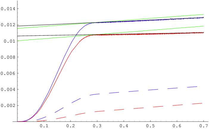
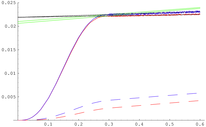
In Fig. 3, we compare the energy loss at for different masses but equal velocity at the time when the external force is set to zero. The curves have essentially constant slope for , meaning that the rate of energy loss is nearly constant in the limited time window that we have access to. The lines in the figure contrast the instantaneous rate of energy loss in this interval, obtained by a numerical fit and denoted henceforward by , against the corresponding stationary result of [7, 8], which we will denote by . For , is close to two times bigger than , and as the value of decreases (corresponding to heavier quarks), the difference between the two rates grows bigger. In particular, for , is at least three times bigger than .


A similar comparison is shown is Fig. 4, but with a fixed mass value and different release velocities. In all cases, we have found again that the rate of energy loss (37), valid in the stationary regime, is above our numerical result. The discrepancy observed is significantly larger than our estimated margin of error. Our results therefore provide clear evidence that, in the mass range of primary phenomenological interest, there exist conditions under which the rate of energy loss for a heavy quark that moves only under the influence of the plasma can be substantially smaller than the rate obtained in [7] for the steady-state or late-time configuration. We will return to this point in Section 5.4.
As one would expect, the numerical rate of energy loss depends on and . As shown in Fig. 5, for fixed mass values, it varies quadratically with the velocity of the quark. As we had mentioned before, for the small velocities that we can attain, we must deal only with the non-relativistic approximation of the dispersion relation (56). This implies that the accumulated energy loss (55) varies quadratically with the quark velocity , and so the constant slope that we are reading off of the portion of the numerical curves in Figs. 3 and 4 should be proportional to , where denotes the small change in velocity in the given time interval. The parabolic behavior seen in Fig. 5, then, tells us that . In other words, in the leading non-relativistic version of (49), the friction coefficient is independent of the quark velocity, as one would expect.
Unfortunately, due to limitations with the numerical integration, we have not been able to characterize the dependence of the dissipation rate on the mass of the quark, beyond the statement that increases roughly linearly with increasing (decreasing ). In particular, above , the numeric rate becomes indistinguishable (within our margin of error) from the stationary result (37).


Let us now consider the initial stage . From the beginning portion of the curves in Figs. 3 and 4, we can see that the situation when the quark is subjected to an external force is opposite to what we described above for unforced motion: the rate at which energy is dissipated can be substantially larger than (37), suggesting that in this segment of the quark trajectory the mechanism of energy loss is qualitatively different. In particular, the energy lost in this region is by no means negligible, which is precisely the obstacle that prevents us from directly inferring the quark’s dispersion relation from our numerical results, as envisioned in [7]. We had anticipated this already in the discussion above, based on our results for the case in Section 2.
When, using the numerical data of the evolution within the plasma, we compare as in Fig. 6 the energy lost by the heavy quark, Eq. (55), against the modified Lienard formula (18), we find that for the two curves are virtually indistinguishable from one another when , , and, to a lesser extent, . In fact, this approximate agreement continues to hold (albeit somewhat reduced) even if in (18) we plug in the data of the quark trajectory at zero temperature. In other words, for quark masses in the phenomenologically interesting range, the quark behaves initially as if there were no plasma, and loses energy through radiation, at a rate equal to the modified Lienard formula given by the first term in (18). This is of course as one would expect from the gauge theory perspective, for a heavy quark should indeed be insensitive to the plasma for very early times.
On the gravity side, the issue is that, for these relatively low values of , the factor of is so close to unity that the modifications induced by the black hole horizon on and only become appreciable when a sufficiently large time has elapsed. We should emphasize that it is not possible to reproduce the numerical results for and in this initial stage using the dispersion relation (46) and dissipation rate (37) derived in [7] (the values of the latter are indicated by the dotted curves in Figs. 3-4).
Beyond the curves in Fig. 6 separate, showing the influence of the hot medium, although somewhat diminished compared to the stationary result (37), as we know from Figs. 3-4. Since it was shown in [7] that (37) will hold at asymptotically late times, we expect the rate of energy loss seen in Figs. 2-6 to increase as the system evolves further. Regrettably, with our very limited integration time we are not able to track the evolution far enough to locate the characteristic transition time to the asymptotic behavior. We will return to this issue from a different perspective in Section 4.4.
3.3 Late-time behavior and worldsheet black hole
It is interesting to visualize the evolution of the system beyond the limited time interval covered by our numerical data, in parallel with our discussion for the zero-temperature case in Section 2.3. The quark, initially static, and accelerated by an external force between (originally ) and , will thereafter decelerate under the influence of the plasma, approaching rest at some location as . In the dual gravity description, this means that the final string embedding, just like the initial () one, must include a static vertical segment extending all the way from the D7-branes at to the black hole horizon at , to represent the quark at rest.
As time progresses, the lower () string endpoint traces out the trajectory of the quark, moving from to . The upper () endpoint, on the other hand, remains at for all finite times, because the wavefront generated on the string by the acceleration of the bottom tip will reach the spacetime horizon only at . Given these boundary conditions, on the - plane the string will clearly evolve from purely vertical to -shaped, with a horizontal segment at , extending from to . All of the energy (and momentum) lost by the quark throughout its evolution ends up in this top portion of the string, which encodes the IR region of the gauge theory. The region of no escape is bounded as in Section 2.3 by a worldsheet horizon that can be identified by standing on the corner of the string and projecting back along the downward-pointing light half-cone , now defined by
| (57) |
The resulting curve descends from before , reaches a minimum value of the radial coordinate, and then moves up again, finally approaching the ‘corner’ as . The upward segment lies fully within the maximally-disturbed region of the worldsheet, located between the upward null curves and obtained by integrating (57) with the upper choice of sign and with initial condition or , respectively. A lower bound on the location of the upward portion of is given by the (upward segment of the) stationary limit curve , defined as the locus where , i.e., . The situation is summarized in Fig. 7.

If, instead of releasing the quark, we pull it with constant velocity for an arbitrarily long period of time (i.e., if ), then we approach the steady-state configuration of [7, 8], and in so doing stabilize the worldsheet horizon (as well as the stationary-limit curve) at , just like in [20, 19] (and [29]).
The behavior of the string long after was determined quantitatively in [7], and is of the form , with the friction coefficient given by the lowest quasi-normal frequency. It was shown there that the imposition of a purely ingoing boundary condition near the spacetime horizon forces the string to deviate from the vertical by a divergent amount ( as ). This is consistent with the development of a ‘corner’, just as we have argued above for the case where the quark is initially static.
Just as we found at , we see here that energy dissipation seems to be irrevocably tied to the appearance of a worldsheet black hole. Since our numerical results show that the initial energy loss is controlled by a friction coefficient , it would appear like in the unforced case the asymptotic rate sets in only when the string is sufficiently close to its final shape. It would be interesting to establish a more detailed connection between the instantaneous rate of energy dissipation from the quark and the rate at which energy crosses the worldsheet horizon, generalizing the results of [20, 19] for the stationary configuration.
4 Quark-Antiquark Evolution
A string with both of its endpoints on the D7-branes describes a quark-antiquark pair. The situation that is closest to modeling the dual process of primary phenomenological relevance, where a heavy quark and antiquark are created within the plasma at time and then separate from one another, is such that the string endpoints start out with coincident positions but different velocities. In a first exploration of this system, it is interesting enough to consider the simple case where the string endpoints are taken to separate back-to-back with the same initial speed , meaning that the pair’s center of mass frame coincides with the plasma rest frame. We will let denote the direction of motion.
4.1 Review of earlier results
A numerical study of this problem was carried out in [7]. It was found that the quark and antiquark trajectories can be more efficiently followed to later times if instead of describing the string embedding in the obvious static gauge , one astutely chooses worldsheet coordinates for which the constant slices manage to reach larger values of near while staying away from the horizon at . This is most easily implemented by working with the Polyakov (rather than Nambu-Goto) action
| (58) |
with the intrinsic metric on the string worldsheet, and making the non-standard gauge choice , , . The ‘stretching factor’ implicitly defines our choice of worldsheet coordinates, and is meant to be adjusted by hand to keep the numerical integration away from the horizon for the longest possible time. For a given trajectory, it is the function that determines the proximity to the horizon, so this goal is achieved by setting (at the level of the equations of motion). Following [7] we will use in the examples below.
In this setting, the evolution of the string is controlled by the equations of motion
| (59) | |||||
(where , ,) supplemented with the constraints
| (60) | |||||
which as always amount to the statement that the intrinsic metric on the worldsheet must be proportional to the induced metric (thereby establishing the classical equivalence with the Nambu-Goto formalism). Given initial data that satisfy (60), the requirement that the constraints continue to hold throughout the evolution gives an important consistency check on the numerical integration. The results we will report throughout this section were obtained with Mathematica 5.2’s NDSolve integration routine, with the constraints typically satisfied at the or level.
In terms of the momentum densities , we see that, as usual, the first two equations in (59) express the conservation of the Noether currents and , respectively associated with invariance under translations in and . To describe a quark-antiquark pair that is not acted upon by any agent other than the plasma, we must choose the standard Neumann/Dirichlet boundary conditions
| (61) |
The total energy
| (62) |
and -momentum
| (63) |
of the string are then conserved.
For the problem at hand, the authors of [7] identified a one-parameter family of initial conditions that correctly satisfy the constraints (60) and are compatible with the boundary conditions (61). Working from now on in units where , these conditions take the form
| (64) | |||||
and describe a string that is pointlike at and grows for as a result of its non-zero initial velocity
| (65) |
The parameter (which has been rescaled here by a factor of with respect to [7]) controls the energy (62) of the configuration,
| (66) |
As expected, the total -momentum vanishes.
Using the initial conditions (64), it was found in [7] that, depending on the value of , the subsequent behavior of the string endpoints can be of two different types. When the energy of the pair is large enough (essentially, ) the quark and antiquark move apart and are able to escape from one another’s influence, so they simply slow down monotonically until they are finally (at ) brought to rest by the plasma. For low , on the other hand, the mutual attraction of the quark and antiquark manages to stop them and make them reverse direction, after which they undergo a number (larger than one quarter) of oscillations before dissipating all of their energy to the plasma. During consecutive half-cycles the body of the string is alternately above and below the line, as a result of which the corresponding motion is asymmetric.66 6 Configurations where the string lies below its endpoints have been considered previously in [29, 30]. In such circumstance, one suspects that the string would prefer to shrink by sliding its endpoints along the D7-branes, moving them closer to the boundary and to each other. To examine this question, however, one must remember: first, that the boundary conditions for the string are purely Neumann or Dirichlet only when the D7-brane embedding is described in the original Cartesian coordinates, and are actually mixed in the spherical coordinates that are naturally employed after taking the AdS/CFT limit; second, that the string coordinates on the describe the internal degrees of freedom of the quark, which one may or may not wish to fix externally.
4.2 Generalized initial conditions
Intuitively, it should be possible to generalize the initial velocity profiles (65) proposed in [7] to more general functions , , which amounts to stipulating that , . Based on the symmetry of our problem, for simplicity we restrict attention to functions that are odd on the interval . Compatibility with the Neumann boundary condition in (61) requires that , the Hamiltonian constraint in (60) determines in terms of , and the Dirichlet boundary condition in (61) demands that . Altogether, then, we find that we are allowed to choose
| (67) | |||||
with and , which constitutes an infinite-parameter generalization of the initial conditions (64).
The energy of all of these configurations is given by the same formula (66). Since the string is initially a point, it might seem peculiar that one can physically distinguish among various possible velocities for its different ‘internal points’— one might suspect that the seemingly different initial profiles (67) are all related to each other by gauge transformations. That this is not the case can be seen most straightforwardly by evolving a few of these initial configurations forward in time: as shown in Fig. 8, the resulting spacetime trajectories are found to be distinct. Notice in particular that in the dashdotted trajectory the quark actually reverses direction before coming to rest, which shows that the boundary between oscillatory and non-oscillatory behavior depends strongly on the way in which the gluonic field (dual to the string) is excited. So the moral of the story is that, while the string is initially a point in spacetime, it is most definitely not a point in phase space, and it is this fact that allows the existence of a truly infinite-dimensional family of initial conditions.


The question of the gauge-dependence of our description does however serve to highlight a useful point: instead of sampling different initial conditions by varying the functional form of in (67) (for a fixed choice of the worldsheet coordinate ), we can keep the form of fixed and change the meaning of . One way to do the latter is to modify our choice of the initial stretching factor . It is easy to see that this indeed leads to different spacetime trajectories, even if the initial energies (66) are appropriately matched. Conversely, when tweaking to find the choice that optimizes the numerical integration for a given physical string configuration, one must keep the initial stretching factor fixed, to ensure that the initial conditions for the evolution do not change. For our calculations we found it convenient to use , with adjustable .
It is natural to wonder what the interpretation of the different initial conditions (67) is in the dual SYM language. The answer is provided to us by the standard recipe for correlation functions [2]: different time-dependent string profiles correspond to different time-dependent configurations of the gluonic fields [56, 41]. Just like the string embedding is not completely characterized by giving the location of its endpoints, the initial state of the gauge theory is not uniquely characterized by specifying the position of the quark and antiquark. This is of course true already in zero-temperature QED, but in that case the linear character of the equations of motion makes it easy to identify, for a given field configuration, the portion that is directly ascribable to the sources of interest.
Notice from (67) that the initial velocity of the quark, , is not a free parameter of the system, but is uniquely fixed by the choice of , or equivalently, by the quark’s Lagrangian mass , according to (28). The reason for this is easy to understand on the string theory side. At , the pointlike string happens to obey not only , in compliance with (61), but also , according to (67), as would befit an endpoint that is free in all spacetime directions. It is well-known that the endpoints of such a string must move at the speed of light (see, e.g., [61]), and, given that the endpoints are located at , we see from (1) that, indeed, a coordinate velocity corresponds precisely to a proper velocity , a fact that was first pointed out in [35].77 7 The same reasoning in fact applies to ‘all points’ on the string: their proper initial velocities clearly satisfy , independently of the choice of . In the gauge theory, this identification confers then a special status to the mass-dependent velocity
| (68) |
whose meaning will be discussed further in the next subsection.
At least from the gauge theory perspective, one would expect to be able to find configurations in which the initial quark velocity is freely adjustable. Given the discussion of the previous paragraph, we see that on the AdS side this can be achieved with initially coincident string endpoints only if we choose . To satisfy the first constraint in (60) we must then set . Picking for the string a velocity profile that is an arbitrary odd function on the interval , the complete second set of allowed initial conditions is then
| (69) | |||||
with an even function on the interval, which satisfies for compatibility with the Dirichlet boundary condition in (61), and
| (70) |
to comply with the Hamiltonian constraint in (60). By construction, the initial quark velocity can now be chosen arbitrarily, as long as in order for the right-hand side of (70) to be real at . The energy (62) of the configuration is now given by
| (71) |
The linear momentum is still zero.
Conditions (69) describe a linelike string that extends purely along the radial AdS coordinate, stretching upward from up to some turning point and then returning back down to . The function will be smooth at the turning point only if , which combined with (70) and the requirement implies that , i.e., the string turns around at the horizon. For this to occur, given an initial velocity profile , the value of must be tuned in order for the numerical solution of (70) to reach precisely at . So for these initial conditions, where is a free parameter, is not. Having determined , one can proceed as before to the numerical integration of the equations of motion (59). A few representative quark trajectories are shown in Fig. 9, with and (chosen to simplify the equation of motion and increase the stability of the numerical integration needed to obtain the initial profile ).

The existence of the two qualitatively distinct sets of initial conditions for the string describing the creation of a quark-antiquark pair has a direct field-theoretic interpretation: the product of a fundamental and an antifundamental can lead to a - pair either in the singlet or the adjoint representation of the gauge group, and each of the above string configurations is dual to one of these. Indeed, the linelike string (69) is precisely the system considered in [45, 37, 62, 18] to model a color source in the adjoint representation. Due to its extended nature, it sets up long-range supergravity fields that translate through the standard recipe of [2] into a long-range gluonic field profile, indicative of a source with net color charge. The completely pointlike string (67), on the other hand, sets up no long-range chromoelectromagnetic field and so describes the singlet. Given this correspondence, it is interesting that the AdS/CFT duality predicts that (at large and large ) the initial quark velocity is freely adjustable in the adjoint, but not the singlet, configuration.
4.3 Limiting velocity
In the previous subsection we have learned that the initial velocity of the quark and antiquark at the moment of the pair’s creation is bounded above by the speed defined in (68). The reason for this is easy to understand on the string theory side of the duality, since, as we have noted above, the coordinate velocity corresponds to a proper velocity equal to that of light at the position of the string endpoints, [35]. The interesting feature is that it is , and not , that corresponds to the gauge theory velocity.
We would naturally expect the restriction to subluminal velocities, , to apply to more general string configurations. In complete analogy with the point particle case, the easiest way to deduce this restriction is to go back to the Nambu-Goto action (2), and observe that the requirement that it be real (i.e., that the string worldsheet be timelike) imposes a bound on physically realizable embeddings. Indeed, working for simplicity in the static gauge , it is easy to see that the Nambu-Goto square root is real only as long as the embedding function satisfies
| (72) |
where . For a string that moves and stretches along a single direction , as we have considered up to now, or and this reduces to
| (73) |
It might seem peculiar that, as long as the string segment under consideration is not vertical (), the bound (73) allows the proper velocity of the segment, , to exceed the speed of light (by an amount that becomes arbitrarily large in the limit ). One should note, however, that this is a gauge-dependent statement, because unless the string segment is vertical, is not entirely transverse to it, and the longitudinal component of the string motion is of course unphysical (in particular, motion along is entirely unphysical in the limit , where the string becomes horizontal). From (72) we can see that, for purely transverse motion, (as in the meson configurations we will consider in Section 5), the proper velocity is indeed required to be less than unity, i.e., the coordinate (or, equivalently, gauge theory) velocity is bounded by .
The argument of the preceding paragraph applies to a generic point in the interior of the string, but the situation is different for the endpoints, where motion along the body of the string is physical. As we know, a string endpoint on the D7-branes is dual to a quark (or antiquark), so the velocity of the latter must necessarily respect the bound (72), or, for collinear motion, (73). Evaluating this last equation at and parametrizing as in Sections 2 and 3 the -dependence in terms of the momentum density given by (3), which controls the external force applied to the quark, we deduce that is bounded by
| (74) |
where and denotes the expression within brackets in (28).
For the case we have considered in the previous two subsections, where the string endpoint is free, corresponding to a quark that evolves only under the influence of the plasma, (74) is precisely the statement that . As expected, we see that this bound (or, more generally, the analogous bound deduced from (72)) applies not only to quark-antiquark configurations, but also to isolated quarks.88 8 This observation has also been made very recently in [30]. Simultaneously, has been shown to emerge as a limiting velocity directly from the microscopic meson dispersion relation [39]. Both of these works appeared while the present paper was in preparation.
For the case where the quark is externally forced, on the other hand, the bound (74) becomes less restrictive: as increases, the quantity on the right grows monotonically, and in fact diverges when the force approaches the critical value mentioned already in Section 3.2 (this is the same as the divergence seen in (72) and (73) when ). From this perspective alone, then, it would seem possible to take the quark to velocities larger than while exerting a force on it (even though, after release, one would again have ).
It is not guaranteed, however, that this possibility is realized in practice. In the forced stationary case considered in [7, 8], for instance, it is found that would necessarily require , and is consequently unattainable [20]. More generally, the question of whether is limiting or not is dynamical in nature, and essentially depends on the form of the thermal dispersion relation for the quark. In the discussion following (52) we noted that, based on our zero-temperature results of Section 2, the quark’s intrinsic energy (and momentum ) should diverge as . Given the connection between the factor in the denominator of (52) and the Lorentz invariance of the metric (1) at , it is natural to expect it to be replaced by at finite temperature, which would imply that (and ) as , meaning that is physically unattainable. The results we will obtain in Section 5.3 appear to support this expectation, but it would certainly be nice to be able to show this directly.99 9 For mesons this was done recently in [39], which appeared while this paper was in preparation.
4.4 Transition to asymptotic regime
For the non-oscillatory string trajectories with the one-parameter family of initial conditions (64), it was found in [7] that the late-time quark motion is independent of the energy of the configuration, and coincides with the behavior expected from a particle with relativistic dispersion relation , subject to a damping force
| (75) |
with a -independent friction coefficient that was tabulated in [7] for various values of , and which is consistent with the drag force (37) obtained in [7, 8, 9] for the stationary configuration.
The agreement between the analytic and late-time numeric results is most cleanly seen if instead of comparing graphs of or for the quark (where one would need to look at ), one examines the plots of ,1010 10 We thank Antonio García for suggesting this. where the analytic behavior for constant takes the simple form
| (76) |
which is linear with slope near the final rest point (whose value is meant to be adjusted to fit the data). These plots are shown in Fig. 10, where it is seen that the late-time behavior is well-described by (76) also for oscillating trajectories and for the more general singlet configuration (67), as well as for the adjoint configuration (69). Notice that the agreement holds in the late-time regime where (76) reduces to a linear expression, but, as in the cases studied by the authors of [7], it extends beyond the range covered by their general quasi-normal mode analysis, because the velocity of the quark is not necessarily small.

In Fig. 10, we see that there is an initial period where the behavior differs from the late-time frictional evolution (76). This difference is clearly more significant for the singlet than the adjoint case. The time that must elapse before the asymptotic behavior sets in becomes arbitrarily large for singlet configurations that are close to being oscillatory. In these cases, essentially all of the energy of the quark is lost not through the constant- frictional force due to the plasma, but as a result of the chromoelectromagnetic force exerted by the antiquark.
On the string theory side of the duality, the issue is that, as the initially pointlike string grows and falls toward the black hole, it takes some time before it is close enough to to be deformed into (two juxtaposed copies of) the asymptotic shape discussed in Section 3.3. This picture seems rather close to the phenomenological discussion given in [50] (in the context of collisional energy loss): when the singlet quark-antiquark pair is formed within the plasma, there is a delay before the interaction between the newly created sources and the plasma can set up the long range gluonic field profile that is responsible for the late-time dissipation.
To examine in more detail the transition to the late-time behavior (76), for a variety of trajectories we have determined the point beyond which the numeric curve agrees with the analytic curve (76) to the accuracy indicated by the fraction . Even though, judging by the effect of halving the grid spacing, our numerical results seem to be accurate to at least 1%, the precision with which we can determine is limited by the uncertainty in the fitting parameter , which we estimate to be of order 5-10%. It does not make much sense therefore to consider a value of smaller than this.
A representative sample of our results for and , in the case of singlet configurations is shown in Fig. 11. The two sets of data have somewhat different functional forms, but are consistent with one another within the rather large margin of error. The general tendency is for to approach zero as .
For adjoint configurations, we find that the numeric curves are within 5-10% of (76) already at the start of the evolution, so, to be consistent with our pre-established criterion, in this case we must identify the transition length as essentially . It is still worth noting, however, that there is an initial period where the functional form of the numeric and analytic plots is different, as can be seen in Fig. 10. This difference is negligible for small initial velocities, and becomes more pronounced (both in magnitude and in duration) as increases. The transition length identifiable at the 3-4% level thus follows a trend opposite to the one for the singlet case. Nonetheless, up to the velocities that we have been able to explore (corresponding to ), it remains smaller than the singlet shown in Fig. 11.

A question worth considering is whether the transition to the regime where the quark experiences a constant drag coefficient occurs right after the quark and antiquark are screened from each other by the plasma, or if there is an intermediate regime where the quark moves independently from the antiquark but nevertheless feels a drag force that differs from the stationary result of [7, 8, 9], as we found when applying an external force in Section 3.2. To answer this question, we will determine the relevant screening length in the next section.
It would also be very interesting to develop an interpretation of energy loss for the evolving quark-antiquark pair in parallel with the picture for an isolated quark proposed by Mikhailov [52] and developed further in Sections 2,3. An effort in this direction was in fact made in the work [63], but regrettably we do not understand its use of trajectories that lie outside of the string worldsheet. We suspect that a treatment based on null curves on the worldsheet should be possible. Of course, progress is again hampered by the lack of an analytic solution describing the back-to-back - evolution considered in this section (or even its counterpart at zero temperature). Another potentially confusing issue is the fact that, in contrast with the isolated quark case, there are now two string endpoints at , and a priori it would be possible for null trajectories to ‘bounce’ repeatedly between them. One should however bear in mind that, at least beyond some finite interval of time, this would be prevented by the formation of a worldsheet horizon analogous to the one discussed in Sections 2.3,3.3.
5 Quark-Antiquark Potential
5.1 Review of earlier results
The potential for an infinitely massive static quark and antiquark in a strongly-coupled SYM plasma was determined in [64],1111 11 For the corresponding weak coupling calculation in QCD, see, e.g., [66] and references therein. using the dual description of the pair in terms a string with both of its endpoints on the AdS boundary . As expected, for small quark-antiquark separation , the effects of the plasma are negligible and the potential matches the zero-temperature result [65]
| (77) |
As the separation grows, however, the effects of the plasma progressively screen the quark and antiquark from one another, and as a consequence raise the system’s energy above the Coulombic behavior. The -shaped string embedding that is employed for the calculation exists only up to a maximal separation , and its energy exceeds that of the disconnected solution beyond the somewhat smaller distance . In the limit where the string-theoretic calculation is easy to carry out, the potential has a kink at , and beyond this point the string path integral is dominated instead by a configuration with high worldsheet curvature which for large describes graviton exchange between two disconnected strings, leading to a tail , with [38].
This computation can easily be extended to the case where the - pair moves with velocity with respect to the plasma, to obtain the energy of the pair [28, 27]. For any , the potential reduces to (77) at small . The main overall effect of increasing the velocity is to move the non-Coulombic portion of the curve down and to the left, leading in particular to the identification of the two screening lengths for .
The function was determined numerically in [32, 28] (and a related length was plotted in [31]).1212 12 The works [32, 27] additionally explored the dependence of on the angle between the direction of motion and the dipole axis (which was fixed at in [28]), finding it to be weak. Over the entire range its behavior may be approximated as [28]
| (78) |
while in the ultra-relativistic limit, it can be shown analytically that [32]
| (79) |
The full curve does not deviate far from this asymptotic form, so a decent approximation to it is obtained by replacing in (80), to reproduce the correct value at (at the expense of introducing a 16% error as ) [32]:
| (80) |
A comparison between the two approximations (78) and (80) is shown in Fig. 12: overall, the exponent is better than in the sense that it implies a smaller squared deviation from the numerical results, even though leads to a smaller percentage error in the range (). An attempt to better parametrize the deviation away from the ultra-relativistic behavior was made in [36]. In any case, one should bear in mind that the region of principal interest at RHIC is not really , but (see, e.g., [67]).

It is interesting to consider how these results generalize to the case where the quark and antiquark have a large but finite Lagrangian mass , which as reviewed in Section 2 corresponds to letting the flavor D7-branes extend up to a position given by (28). As explained in Section 3.2, from the phenomenological perspective we are mostly interested in values of the mass parameter in the range , which corresponds to the charm mass.
5.2 Finite mass at zero temperature
In a static configuration, the equation of motion for the string amounts to the statement that the momentum density given by (3) is independent of . In the pure AdS geometry (i.e., in the metric (1) with ) the resulting embedding is [65]
| (81) |
where denotes the turning point of the -shaped string and the plus or minus sign applies respectively to its right and left half. From this it follows in particular that the distance between the string endpoints at (i.e., the - separation) is
| (82) |
where denotes the incomplete Euler beta function. The energy of the -shaped string, renormalized by subtracting the energy of two purely radial strings, follows from (2) as
| (83) |
The corresponding results for the case of a moving - pair are of course determined in terms of these by Lorentz invariance.
Using (82) and (83), it is easy to see that for (i.e., ) the quark-antiquark potential approaches the same Coulombic form (77) as in the infinitely massive case (). On the other hand, in the short distance limit we have and so the potential is linear,
| (84) |
These results are consistent with the form of the gluonic field around an isolated finite-mass quark [59],
| (85) | |||||
(where denotes the operator dual to the dilaton field [68]), which is Coulombic at long distances and non-singular at the location of the quark.
In both (84) and (85) we are seeing the effect of a color charge distribution that cloaks the fundamental sources, or in other words, of the gluon (and scalar, etc.) cloud that surrounds the would-be bare quark to turn it into a ‘dressed’ or ‘composite’ quark, in line with the inferences we made in Section 2.2. Notice from (85) that the size of this cloud is not the Compton wavelength of the quark, (indicating that it is not made of virtual quarks and antiquarks), but the much larger scale , which is the characteristic size of the deeply bound microscopic mesons of the theory [69, 70, 59]— so perhaps it would be more appropriate to refer to this charge distribution as a ‘meson cloud.’
5.3 Finite mass at finite temperature
We will consider first the case where the quark-antiquark pair is static with respect to the plasma. Repeating the calculation of the previous subsection for , the separation between the quark and antiquark is found to be
| (86) |
with , and the renormalized energy of the pair is given by
| (87) |
From (86) and (87), the short-distance behavior of the potential is now
| (88) |
with related to the quark Lagrangian mass through (28). By comparing with numerical plots (as in Fig. 13 below), this linear expression can be seen to give a good approximation of the actual potential at least up to .
The constant term in (88) is clearly nothing but (minus) the thermal rest mass (38) of the isolated quark and antiquark, which was subtracted in our choice of renormalization. For any , the force deduced from the potential balances the external force
| (89) |
required to hold the string endpoint in place, and the coefficient of the linear term in (88) correctly encodes the () limit of this force. Using (1) and (68), this can in turn be rewritten in the form
| (90) |
which coincides with the drag force (37) computed with a trailing string in [7, 8], evaluated at the velocity . This agreement has a simple interpretation. As explained in [20], the drag force calculation of [7, 8] has a limited range of validity ( for a given , or equivalently, for a given ), arising from the condition that the electric field needed to keep the string endpoint moving at constant speed does not exceed its critical value at , . This critical electric field is thus equivalent to the maximal attainable drag force, . The fact that it agrees with the right-hand side of (90), then, is not surprising, because, by definition, encodes the force needed to pull apart the endpoints of a zero-size string at , i.e., the value of . In gauge theory language, this is the force required to nucleate a quark-antiquark pair.
For , the potential is screened and deviates significantly from the linear form (88). Its behavior is shown in Fig. 13. As can be seen there, the location of the screening lengths and shift to the left with increasing (e.g., for we respectively find and ).

Let us now go on to consider the case where the quark-antiquark pair moves through the plasma. For simplicity, as in [28] we will restrict ourselves to the case where the motion is perpendicular to the dipole axis (other angles have been studied in [32, 36, 27]). Orienting the former along and the latter along , the expression for the - separation can be copied directly from Eq. (37) of [28]. It is given by
| (91) |
where
is a rescaled version of the force needed to hold the quark and antiquark in place, is the function appearing in the metric (1),
| (92) |
and we have taken into account the finiteness of the quark Lagrangian mass by changing the upper limit of the integration range from 1 to . The form of expression (91) reflects the fact that, in spite of its motion with respect to the black hole, the string remains completely vertical, in contrast with the trailing configuration studied in [7, 8]. In the gauge theory, this translates into the interesting property that, unlike isolated quarks, mesons feel no drag [31, 32, 28].
Similarly, the energy of the - pair in its rest frame1313 13 For a discussion of subtleties in the calculation of the pair energy in the rest frame of the plasma, see [28]. can be read from Eq. (38) of [28] as
| (93) |
The second term in this expression represents the energy of two disjoint strings trailing their boundary endpoints as in [7, 8], dual to an unbound quark and antiquark (which do experience a drag force). This contribution is subtracted in order for to correspond to the energy beyond which the system would become unbound.


Carrying out the integrals in (91) and (93) numerically, one obtains plots for the potential such as those shown in Fig. 14. For small separation the behavior is again linear,
| (94) |
The two terms in this expression have the same interpretation as was given for (88) in the paragraph surrounding (89)-(90).
From Fig. 14 one also sees that the value of has an effect on the location of the screening lengths , (and the velocity beyond which ). The behavior at fixed and varying shown in Fig. 14a is qualitatively the same as we saw already for the static configuration in Fig. 13. The dependence at fixed and varying , which is more relevant for the phenomenological situation, is shown in Fig. 14b.


In Figs. 15 and 16, we see that when , and to a lesser extent, when , the screening length is still relatively well approximated in the full range by the natural modification of the fit (78),
| (95) |
This approximation becomes worse as is further increased. (In all cases, the fit analogous to (80),
| (96) |
does a poorer job than (95).)


An important difference with respect to the case where the quarks are infinitely massive is that now the ‘ultra-relativistic’ region would refer to the limit where the pair velocity approaches the limiting velocity given in (68) and discussed further in Section 4.3. From this alone it is clear that the asymptotic formula (80) no longer holds. The behavior in this region can still be determined analytically, and turns out to be
| (97) |
where we see that the exponent in (79) changes to at finite quark mass. As shown in Figs. 15b and 16b, for values of in the neighborhood of the charm mass, the functional form (97) applies only for velocities extremely close to the endpoint. As is further increased, however, there is a tendency for (97) to apply to a larger fraction of the interval.
In [32, 27], the result (80) for the screening length in the infinitely massive case was turned into a tentative prediction for the dissociation temperature of charmonium or bottomonium traversing the quark-gluon plasma, . (As reviewed in Section 4.1, for the exponent implied by the AdS/CFT calculation is really closer to than to .) The argument for this velocity scaling is heuristic, and relies on comparing the screening length against the natural size of the bound state in question (see, e.g., [71] and references therein). Applying the same logic to the fits (95) or (97) for the screening length in the case of masses in the neighborhood of the charm quark ( 0.2-0.4, as in Figs. 15-16), one would infer that , with for general , and in the limit (the latter being the preferred fit only in the restricted range or , depending on the value of ).
While this paper was in preparation, the work [39] appeared, which includes an explicit derivation of the dispersion relation for mesons, described as open string modes on the D7-branes, following [69]. For large meson momentum , their calculation resulted in , with the limiting velocity defined in (68) and discussed further in Section 4.3 of the present paper (as well as in [30], which also appeared while our work was being written up). The authors of [39] emphasized that the - and -dependence of implies a bound on the temperature at which a meson with velocity can exist within the plasma. Interpreting the maximal allowed temperature as a dissociation temperature, they found the scaling , just like the heuristic argument based on the potential for infinitely-massive and ultra-relativistic quarks had suggested [32, 27].
Given the results of [28] and the present subsection, we are not quite sure what to make of this agreement. As explained above, for finite mass the quark-antiquark potential does not scale as even in the ‘ultra-relativistic’ region (which is now ). So the fact that the heuristic argument in [32, 27] based on the potential suggests the same scaling with velocity as the direct calculation in [27] might be a coincidence, or it might indicate that there is a direct physical connection between the dissociation temperature and the potential only when the latter is computed for infinitely-massive quarks. In any case, it should be emphasized that the scaling follows not from the detailed computation of the dispersion relation in [27], but from the temperature-dependence of the limiting velocity (68).
5.4 Screening length vs. transition distance
In Fig. 11 at the end of the previous Section, we determined the location beyond which a quark and antiquark created (with zero total momentum) within the plasma begin to slow down at the asymptotic rate specified by the constant friction coefficient obtained for an isolated quark in [7, 8]. For - separations larger than , then, the two particles are definitely oblivious to one another and evolve independently. It is therefore interesting to compare the transition distance against (half of) the screening length determined in the present section, which gives a measure of the minimal distance at which the quark and antiquark can decouple.
For singlet configurations, the result of this comparison is shown in Fig. 17, where we see that the two separations are of comparable magnitude and scale with velocity in a similar manner.1414 14 A similar agreement was reported very recently in [40], which appeared while this paper was in preparation. Notice that this is in spite of the fact that the two relevant string configurations are quite different, with motion respectively along and perpendicular to the plane in which the string extends. We conclude then that the transition to the constant-drag-coefficient regime takes place immediately after the quark and antiquark lose contact with one another. That is to say, unlike what we found for the forced isolated quark in Section 3.2, here there is no intermediate stage where the quark and antiquark decelerate independently from one another at a rate that differs substantially from the asymptotic result of [7, 8].
The initial stage, where as seen in Fig. 10 the quark and antiquark dissipate energy at a rate larger than (37), corresponds to the period when the string has not fallen close enough to the black hole horizon. In other words, to a first approximation, the quark and antiquark evolve in this region as they would in the absence of the thermal plasma. To the extent that this result, with all its simplifying assumptions, might conceivably be extrapolated to the experimental context, this initial stage would not differ significantly between heavy ion and proton-proton collisions.

For adjoint configurations, the quark-antiquark potential is expected to be suppressed by a factor of relative to the singlet case (see, e.g., [72] and references therein). On the string theory side of the duality, this is visible in the fact that the ‘line’ initial conditions (69) can be regarded as describing two disjoint strings extending all the way from the D7-branes to the horizon. In the classical limit where our calculations are carried out, these two halves do not influence one another, because signals propagating between them would have to pass through the horizon, and their splitting/joining/annihilating is suppressed by powers of the string coupling , which is taken to zero. At this level of approximation, then, the quark and antiquark do not see one another, so the relevant ‘screening length’ is . This is consistent with the result we obtained for the adjoint case in Section 4.4.
The fact that in the adjoint case the quark and antiquark evolve independently from the start makes this case directly comparable to our study of isolated quarks in Section 3.2. Interestingly, the corresponding results seem to point in opposite directions: whereas for an initially static quark that is externally forced we identified a short period after release where the quark loses energy at a rate significantly smaller than the stationary/asymptotic rate (37), for a quark that is created with a certain initial velocity and gluonic field profile and thereafter moves only under the influence of the plasma we found an initial rate of dissipation that is somewhat larger than (37).
It seems, then, that the initial conditions can, to a certain extent, influence the subsequent evolution, which does not seem altogether surprising given the nonlinear nature of the medium. The application of an external force in Section 3.2 clearly has a significant effect on the shape of the string at the time of release, or in other words, on the gluonic field configuration surrounding the quark. In view of our results for quark-antiquark evolution in this and the previous section, the initial period over which this disturbed quark behaves unlike what one would expect based on [7, 8, 9] should most likely be interpreted as reflecting the time it takes the quark to stabilize the gluonic fields around it, or, equivalently, to move far enough away from the disturbed region to be effectively screened from it. In any case, one should of course not lose sight of the fact that the actual experimental situation resembles the setup of Section 4 more closely than that of Section 3.2.
Acknowledgements
It is a pleasure to thank Alejandro Ayala, Elena Cáceres, Jorge Casalderrey-Solana, Antonio García and Guy Paic for valuable discussions. We are also grateful to Antonio García for collaboration in the initial stages of this project. We additionally thank Karen Ramírez for help with Figs. 1 and 7. This work was partially supported by Mexico’s National Council of Science and Technology (CONACyT) grants 50-155I and SEP-2004-C01-47211, as well as by DGAPA-UNAM grants IN116408 and IN104503.
References
- [1] J. M. Maldacena, “The large limit of superconformal field theories and supergravity,” Adv. Theor. Math. Phys. 2, 231 (1998) [Int. J. Theor. Phys. 38, 1113 (1999)] [arXiv:hep-th/9711200].
- [2]
S. S. Gubser, I. R. Klebanov and A. M. Polyakov,
“Gauge theory correlators from non-critical string theory,”
Phys. Lett. B 428, 105 (1998)
[arXiv:hep-th/9802109];
E. Witten, “Anti-de Sitter space and holography,” Adv. Theor. Math. Phys. 2, 253 (1998) [arXiv:hep-th/9802150]. - [3] O. Aharony, S. S. Gubser, J. M. Maldacena, H. Ooguri and Y. Oz, “Large field theories, string theory and gravity,” Phys. Rept. 323, 183 (2000) [arXiv:hep-th/9905111].
- [4]
W. A. Zajc,
“The Fluid Nature of Quark-Gluon Plasma,”
arXiv:0802.3552 [nucl-ex];
B. Muller, “From Quark-Gluon Plasma to the Perfect Liquid,” Acta Phys. Polon. B 38, 3705 (2007) [arXiv:0710.3366 [nucl-th]];
E. Shuryak, “Emerging theory of strongly coupled quark-gluon plasma,” arXiv:hep-ph/0703208;
D. d’Enterria, “Quark-gluon matter,” J. Phys. G 34 (2007) S53 [arXiv:nucl-ex/0611012];
C. A. Salgado, “Heavy ions theory review,” Acta Phys. Polon. B 38 (2007) 975 [arXiv:hep-ph/0609172];
E. V. Shuryak, “Strongly coupled quark-gluon plasma: The status report,” arXiv:hep-ph/0608177;
M. J. Tannenbaum, “Recent results in relativistic heavy ion collisions: From ’a new state of matter’ to ’the perfect fluid’,” Rept. Prog. Phys. 69 (2006) 2005 [arXiv:nucl-ex/0603003];
B. Müller and J. L. Nagle, “Results from the Relativistic Heavy Ion Collider,” arXiv:nucl-th/0602029;
M. Gyulassy and L. McLerran, “New forms of QCD matter discovered at RHIC,” Nucl. Phys. A 750, 30 (2005) [arXiv:nucl-th/0405013]. - [5]
K. Adcox et al. [PHENIX Collaboration],
“Formation of dense partonic matter in relativistic nucleus nucleus
collisions at RHIC: Experimental evaluation by the PHENIX collaboration,”
Nucl. Phys. A 757, 184 (2005)
[arXiv:nucl-ex/0410003];
I. Arsene et al. [BRAHMS Collaboration], “Quark gluon plasma and color glass condensate at RHIC? The perspective from the BRAHMS experiment,” Nucl. Phys. A 757 (2005) 1 [arXiv:nucl-ex/0410020];
B. B. Back et al., “The PHOBOS perspective on discoveries at RHIC,” Nucl. Phys. A 757 (2005) 28 [arXiv:nucl-ex/0410022];
J. Adams et al. [STAR Collaboration], “Experimental and theoretical challenges in the search for the quark gluon plasma: The STAR collaboration’s critical assessment of the evidence from RHIC collisions,” Nucl. Phys. A 757, 102 (2005) [arXiv:nucl-ex/0501009]. - [6]
F. Carminati et al. [ALICE Collaboration],
“ALICE: Physics performance report, volume I,”
J. Phys. G 30 (2004) 1517;
A. Morsch [ALICE Collaboration], “Jet quenching studies with the ALICE detector,” Czech. J. Phys. 55 (2005) B333;
L. I. Sarycheva, “Heavy ion collisions at CMS and quark gluon plasma,” Czech. J. Phys. 52 (2002) C171;
D. d’Enterria et al., “CMS physics technical design report: Addendum on high density QCD with heavy ions,” J. Phys. G 34 (2007) 2307. - [7] C. P. Herzog, A. Karch, P. Kovtun, C. Kozcaz and L. G. Yaffe, “Energy loss of a heavy quark moving through supersymmetric Yang-Mills plasma,” JHEP 0607 (2006) 013 [arXiv:hep-th/0605158].
- [8] S. S. Gubser, “Drag force in AdS/CFT,” Phys. Rev. D 74 (2006) 126005 [arXiv:hep-th/0605182].
- [9] J. Casalderrey-Solana and D. Teaney, “Heavy quark diffusion in strongly coupled Yang Mills,” Phys. Rev. D 74 (2006) 085012 [arXiv:hep-ph/0605199].
- [10] H. Liu, K. Rajagopal and U. A. Wiedemann, “Calculating the jet quenching parameter from AdS/CFT,” Phys. Rev. Lett. 97 (2006) 182301 [arXiv:hep-ph/0605178].
- [11]
G. Policastro, D. T. Son and A. O. Starinets,
“The shear viscosity of strongly coupled N = 4 supersymmetric Yang-Mills
plasma,”
Phys. Rev. Lett. 87 (2001) 081601
[arXiv:hep-th/0104066];
A. Buchel and J. T. Liu, “Universality of the shear viscosity in supergravity,” Phys. Rev. Lett. 93, 090602 (2004) [arXiv:hep-th/0311175];
P. Kovtun, D. T. Son and A. O. Starinets, “Viscosity in strongly interacting quantum field theories from black hole physics,” Phys. Rev. Lett. 94 (2005) 111601 [arXiv:hep-th/0405231];
A. Buchel, J. T. Liu and A. O. Starinets, “Coupling constant dependence of the shear viscosity in supersymmetric Yang-Mills theory,” Nucl. Phys. B 707, 56 (2005) [arXiv:hep-th/0406264]. - [12]
A. O. Starinets,
“Transport coefficients of strongly coupled gauge theories: Insights from
string theory,”
Eur. Phys. J. A 29 (2006) 77
[arXiv:nucl-th/0511073];
D. T. Son and A. O. Starinets, “Viscosity, Black Holes, and Quantum Field Theory,” Ann. Rev. Nucl. Part. Sci. 57 (2007) 95 [arXiv:0704.0240 [hep-th]];
R. B. Peschanski, “Quark-Gluon Plasma/Black Hole duality from Gauge/Gravity Correspondence,” arXiv:0710.0756 [hep-ph]. - [13] A. Majumder, B. Muller and X. N. Wang, “Small Shear Viscosity of a Quark-Gluon Plasma Implies Strong Jet Quenching,” Phys. Rev. Lett. 99 (2007) 192301 [arXiv:hep-ph/0703082].
- [14]
R. Baier, D. Schiff and B. G. Zakharov,
“Energy loss in perturbative QCD,”
Ann. Rev. Nucl. Part. Sci. 50 (2000) 37
[arXiv:hep-ph/0002198];
R. Baier, “Jet quenching,” Nucl. Phys. A 715, 209 (2003) [arXiv:hep-ph/0209038];
A. Kovner and U. A. Wiedemann, “Gluon radiation and parton energy loss,” arXiv:hep-ph/0304151. - [15]
J. Casalderrey-Solana and C. A. Salgado,
“Introductory lectures on jet quenching in heavy ion collisions,”
arXiv:0712.3443 [hep-ph];
D. E. Kharzeev, “Theoretical issues in J/psi suppression,” J. Phys. G 34 (2007) S445 [arXiv:hep-ph/0703259];
R. Rapp and H. van Hees, “Heavy Quark Diffusion as a Probe of the Quark-Gluon Plasma,” arXiv:0803.0901 [hep-ph]. - [16]
C. P. Herzog,
“Energy loss of heavy quarks from asymptotically AdS geometries,”
JHEP 0609 (2006) 032
[arXiv:hep-th/0605191];
E. Cáceres and A. Güijosa, “Drag force in a charged SYM plasma,” JHEP 0611 (2006) 077 [arXiv:hep-th/0605235];
S. J. Sin and I. Zahed, “Ampere’s law and energy loss in AdS/CFT duality,” Phys. Lett. B 648 (2007) 318 [arXiv:hep-ph/0606049];
T. Matsuo, D. Tomino and W. Y. Wen, “Drag force in SYM plasma with field from AdS/CFT,” JHEP 0610 (2006) 055 [arXiv:hep-th/0607178];
P. Talavera, “Drag force in a string model dual to large- QCD,” JHEP 0701 (2007) 086 [arXiv:hep-th/0610179];
E. Antonyan, “Friction coefficient for quarks in supergravity duals,” arXiv:hep-th/0611235;
D. Berenstein and H. J. Chung, “Aspects of open strings in Rindler Space,” arXiv:0705.3110 [hep-th];
A. Karch and A. O’Bannon, “Metallic AdS/CFT,” JHEP 0709 (2007) 024 [arXiv:0705.3870 [hep-th]];
C. P. Herzog and A. Vuorinen, “Spinning Dragging Strings,” JHEP 0710 (2007) 087 [arXiv:0708.0609 [hep-th]];
A. O’Bannon, “Hall Conductivity of Flavor Fields from AdS/CFT,” Phys. Rev. D 76 (2007) 086007 [arXiv:0708.1994 [hep-th]];
K. B. Fadafan, “ curvature-squared corrections on drag force,” arXiv:0803.2777 [hep-th];
J. F. Vázquez-Poritz, “Drag force at finite ’t Hooft coupling from AdS/CFT,” to appear. - [17]
E. Cáceres and A. Güijosa,
“On drag forces and jet quenching in strongly coupled plasmas,”
JHEP 0612 (2006) 068
[arXiv:hep-th/0606134];
E. Nakano, S. Teraguchi and W. Y. Wen, “Drag Force, Jet Quenching, and AdS/QCD,” Phys. Rev. D 75 (2007) 085016 [arXiv:hep-ph/0608274];
G. Bertoldi, F. Bigazzi, A. L. Cotrone and J. D. Edelstein, “Holography and Unquenched Quark-Gluon Plasmas,” Phys. Rev. D 76 (2007) 065007 [arXiv:hep-th/0702225]. - [18] M. Chernicoff and A. Güijosa, “Energy loss of gluons, baryons and -quarks in an SYM plasma,” JHEP 0702 (2007) 084 [arXiv:hep-th/0611155].
- [19] S. S. Gubser, “Momentum fluctuations of heavy quarks in the gauge-string duality,” Nucl. Phys. B 790 (2008) 175 [arXiv:hep-th/0612143].
- [20] J. Casalderrey-Solana and D. Teaney, “Transverse momentum broadening of a fast quark in a N = 4 Yang Mills plasma,” JHEP 0704 (2007) 039 [arXiv:hep-th/0701123].
- [21] V. Mazu and J. Sonnenschein, “Non critical holographic models of the thermal phases of QCD,” arXiv:0711.4273 [hep-th].
- [22] C. Athanasiou, H. Liu and K. Rajagopal, “Velocity Dependence of Baryon Screening in a Hot Strongly Coupled Plasma,” arXiv:0801.1117 [hep-th].
- [23] S. S. Gubser, D. R. Gulotta, S. S. Pufu and F. D. Rocha, “Gluon energy loss in the gauge-string duality,” arXiv:0803.1470 [hep-th].
- [24]
P. M. Chesler and A. Vuorinen,
“Heavy flavor diffusion in weakly coupled super Yang-Mills theory,”
JHEP 0611 (2006) 037
[arXiv:hep-ph/0607148];
S. C. Huot, S. Jeon and G. D. Moore, “Shear viscosity in weakly coupled N = 4 super Yang-Mills theory compared to QCD,” Phys. Rev. Lett. 98 (2007) 172303 [arXiv:hep-ph/0608062];
J. P. Blaizot, E. Iancu, U. Kraemmer and A. Rebhan, “Hard-thermal-loop entropy of supersymmetric Yang-Mills theories,” JHEP 0706 (2007) 035 [arXiv:hep-ph/0611393];
W. A. Horowitz and M. Gyulassy, “Testing AdS/CFT Deviations from pQCD Heavy Quark Energy Loss with Pb+Pb at LHC,” arXiv:0706.2336 [nucl-th];
W. A. Horowitz, “Ratio of charm to bottom as a test of pQCD vs. AdS/CFT energy loss,” arXiv:0710.0595 [hep-ph];
W. A. Horowitz, “pQCD vs. AdS/CFT Tested by Heavy Quark Energy Loss,” arXiv:0710.0703 [nucl-th];
S. Caron-Huot and G. D. Moore, “Heavy quark diffusion in QCD and SYM at next-to-leading order,” JHEP 0802 (2008) 081 [arXiv:0801.2173 [hep-ph]]. - [25]
J. J. Friess, S. S. Gubser and G. Michalogiorgakis,
“Dissipation from a heavy quark moving through super-Yang-Mills
plasma,”
JHEP 0609 (2006) 072
[arXiv:hep-th/0605292];
Y. h. Gao, W. s. Xu and D. f. Zeng, “Wake of color fields in charged SYM plasmas,” arXiv:hep-th/0606266;
J. J. Friess, S. S. Gubser, G. Michalogiorgakis and S. S. Pufu, “The stress tensor of a quark moving through thermal plasma,” Phys. Rev. D 75 (2007) 106003 [arXiv:hep-th/0607022];
A. Yarom, “The high momentum behavior of a quark wake,” Phys. Rev. D 75 (2007) 125010 [arXiv:hep-th/0702164];
S. S. Gubser and S. S. Pufu, “Master field treatment of metric perturbations sourced by the trailing string,” Nucl. Phys. B 790 (2008) 42 [arXiv:hep-th/0703090];
A. Yarom, “On the energy deposited by a quark moving in an N=4 SYM plasma,” Phys. Rev. D 75 (2007) 105023 [arXiv:hep-th/0703095];
S. S. Gubser, S. S. Pufu and A. Yarom, “Energy disturbances due to a moving quark from gauge-string duality,” JHEP 0709 (2007) 108 [arXiv:0706.0213 [hep-th]];
P. M. Chesler and L. G. Yaffe, “The wake of a quark moving through a strongly-coupled supersymmetric Yang-Mills plasma,” Phys. Rev. Lett. 99 (2007) 152001 [arXiv:0706.0368 [hep-th]];
S. S. Gubser, S. S. Pufu and A. Yarom, “Sonic booms and diffusion wakes generated by a heavy quark in thermal AdS/CFT,” Phys. Rev. Lett. 100 (2008) 012301 [arXiv:0706.4307 [hep-th]];
S. S. Gubser and A. Yarom, “Universality of the diffusion wake in the gauge-string duality,” arXiv:0709.1089 [hep-th];
S. S. Gubser, S. S. Pufu and A. Yarom, “Shock waves from heavy-quark mesons in AdS/CFT,” arXiv:0711.1415 [hep-th];
P. M. Chesler and L. G. Yaffe, “The stress-energy tensor of a quark moving through a strongly-coupled N=4 supersymmetric Yang-Mills plasma: comparing hydrodynamics and AdS/CFT,” arXiv:0712.0050 [hep-th];
J. Noronha, G. Torrieri and M. Gyulassy, “Near Zone Navier-Stokes Analysis of Heavy Quark Jet Quenching in an SYM Plasma,” arXiv:0712.1053 [hep-ph];
S. S. Gubser and A. Yarom, “Linearized hydrodynamics from probe-sources in the gauge-string duality,” arXiv:0803.0081 [hep-th]. - [26]
A. Buchel,
“On jet quenching parameters in strongly coupled non-conformal gauge
theories,”
Phys. Rev. D 74 (2006) 046006
[arXiv:hep-th/0605178];
J. F. Vázquez-Poritz, “Enhancing the jet quenching parameter from marginal deformations,” arXiv:hep-th/0605296;
F. L. Lin and T. Matsuo, “Jet quenching parameter in medium with chemical potential from AdS/CFT,” Phys. Lett. B 641 (2006) 45 [arXiv:hep-th/0606136];
S. D. Avramis and K. Sfetsos, “Supergravity and the jet quenching parameter in the presence of R-charge densities,” JHEP 0701 (2007) 065 [arXiv:hep-th/0606190];
N. Armesto, J. D. Edelstein and J. Mas, “Jet quenching at finite ’t Hooft coupling and chemical potential from AdS/CFT,” JHEP 0609 (2006) 039 [arXiv:hep-ph/0606245];
Y. h. Gao, W. s. Xu and D. f. Zeng, “Jet quenching parameters of Sakai-Sugimoto model,” arXiv:hep-th/0611217;
A. L. Cotrone, J. M. Pons and P. Talavera, “Notes on a SQCD-like plasma dual and holographic renormalization,” JHEP 0711 (2007) 034 [arXiv:0706.2766 [hep-th]];
Y. h. Gao, W. s. Xu and D. f. Zeng, “Viscosity and jet quenching from holographic model,” arXiv:0707.0817 [hep-ph]. - [27] H. Liu, K. Rajagopal and U. A. Wiedemann, “Wilson loops in heavy ion collisions and their calculation in AdS/CFT,” JHEP 0703 (2007) 066 [arXiv:hep-ph/0612168].
- [28] M. Chernicoff, J. A. García and A. Güijosa, “The energy of a moving quark-antiquark pair in an SYM plasma,” JHEP 0609 (2006) 068 [arXiv:hep-th/0607089].
- [29] P. C. Argyres, M. Edalati and J. F. Vázquez-Poritz, “Spacelike strings and jet quenching from a Wilson loop,” JHEP 0704 (2007) 049 [arXiv:hep-th/0612157].
- [30] P. C. Argyres, M. Edalati and J. F. Vazquez-Poritz, “Lightlike Wilson loops from AdS/CFT,” arXiv:0801.4594 [hep-th].
- [31] K. Peeters, J. Sonnenschein and M. Zamaklar, “Holographic melting and related properties of mesons in a quark gluon plasma,” Phys. Rev. D 74 (2006) 106008 [arXiv:hep-th/0606195].
- [32] H. Liu, K. Rajagopal and U. A. Wiedemann, “An AdS/CFT calculation of screening in a hot wind,” Phys. Rev. Lett. 98 (2007) 182301 [arXiv:hep-ph/0607062].
- [33]
T. Sakai and S. Sugimoto,
“Low energy hadron physics in holographic QCD,”
Prog. Theor. Phys. 113 (2005) 843
[arXiv:hep-th/0412141];
“More on a holographic dual of QCD,” Prog. Theor. Phys. 114 (2006) 1083 [arXiv:hep-th/0507073]. - [34]
E. Cáceres, M. Natsuume and T. Okamura,
“Screening length in plasma winds,”
JHEP 0610 (2006) 011
[arXiv:hep-th/0607233];
S. D. Avramis, K. Sfetsos and K. Siampos, “Stability of strings dual to flux tubes between static quarks in N=4 SYM,” Nucl. Phys. B 769 (2007) 44 [arXiv:hep-th/0612139];
C. Hoyos-Badajoz, K. Landsteiner and S. Montero, “Holographic Meson Melting,” JHEP 0704 (2007) 031 [arXiv:hep-th/0612169];
O. Antipin, P. Burikham and J. Li, “Effective Quark Antiquark Potential in the Quark Gluon Plasma from Gravity Dual Models,” JHEP 0706 (2007) 046 [arXiv:hep-ph/0703105];
M. Natsuume and T. Okamura, “Screening length and the direction of plasma winds,” JHEP 0709 (2007) 039 [arXiv:0706.0086 [hep-th]];
S. D. Avramis, K. Sfetsos and K. Siampos, “Stability of string configurations dual to quarkonium states in AdS/CFT,” Nucl. Phys. B 793 (2008) 1 [arXiv:0706.2655 [hep-th]];
I. Amado, C. Hoyos-Badajoz, K. Landsteiner and S. Montero, “Absorption Lengths in the Holographic Plasma,” JHEP 0709 (2007) 057 [arXiv:0706.2750 [hep-th]];
H. Dorn and T. H. Ngo, “On the internal space dependence of the static quark-antiquark potential in SYM plasma wind,” Phys. Lett. B 654 (2007) 41 [arXiv:0707.2754 [hep-th]];
T. Song, Y. Park, S. H. Lee and C. Y. Wong, “The thermal width of heavy quarkonia moving in quark gluon plasma,” Phys. Lett. B 659 (2008) 621 [arXiv:0709.0794 [hep-ph]];
D. Hou and H. C. Ren, “Heavy Quarkonium States with the Holographic Potential,” JHEP 0801 (2008) 029 [arXiv:0710.2639 [hep-ph]];
K. Peeters and M. Zamaklar, “Dissociation by acceleration,” JHEP 0801 (2008) 038 [arXiv:0711.3446 [hep-th]];
E. Caceres, R. Flauger, M. Ihl and T. Wrase, “New Supergravity Backgrounds Dual to N=1 SQCD-like Theories with ,” arXiv:0711.4878 [hep-th];
K. D. Jensen, A. Karch and J. Price, “Strongly bound mesons at finite temperature and in magnetic fields from AdS/CFT,” arXiv:0801.2401 [hep-th]. - [35] P. C. Argyres, M. Edalati and J. F. Vázquez-Poritz, “No-drag string configurations for steadily moving quark-antiquark pairs in a thermal bath,” JHEP 0701 (2007) 105 [arXiv:hep-th/0608118].
- [36] S. D. Avramis, K. Sfetsos and D. Zoakos, “On the velocity and chemical-potential dependence of the heavy-quark interaction in N = 4 SYM plasmas,” Phys. Rev. D 75 (2007) 025009 [arXiv:hep-th/0609079].
- [37] J. J. Friess, S. S. Gubser, G. Michalogiorgakis and S. S. Pufu, “Stability of strings binding heavy-quark mesons,” JHEP 0704 (2007) 079 [arXiv:hep-th/0609137].
- [38] D. Bak, A. Karch and L. G. Yaffe, “Debye screening in strongly coupled N=4 supersymmetric Yang-Mills plasma,” JHEP 0708 (2007) 049 [arXiv:0705.0994 [hep-th]].
- [39] Q. J. Ejaz, T. Faulkner, H. Liu, K. Rajagopal and U. A. Wiedemann, “A limiting velocity for quarkonium propagation in a strongly coupled plasma via AdS/CFT,” arXiv:0712.0590 [hep-th].
- [40] Y. Hatta, E. Iancu and A. H. Mueller, “Jet evolution in the N=4 SYM plasma at strong coupling,” arXiv:0803.2481 [hep-th].
- [41] C. G. Callan and A. Güijosa, “Undulating strings and gauge theory waves,” Nucl. Phys. B 565, 157 (2000) [arXiv:hep-th/9906153].
- [42] S. Lin and E. Shuryak, “Stress Tensor of Static Dipoles in strongly coupled =4 Gauge Theory,” Phys. Rev. D 76 (2007) 085014 [arXiv:0707.3135 [hep-th]].
- [43]
S. Caron-Huot, P. Kovtun, G. D. Moore, A. Starinets and L. G. Yaffe,
“Photon and dilepton production in supersymmetric Yang-Mills plasma,”
JHEP 0612 (2006) 015
[arXiv:hep-th/0607237];
A. Parnachev and D. A. Sahakyan, “Photoemission with chemical potential from QCD gravity dual,” Nucl. Phys. B 768 (2007) 177 [arXiv:hep-th/0610247];
D. Mateos and L. Patiño, “Bright branes for strongly coupled plasmas,” JHEP 0711 (2007) 025 [arXiv:0709.2168 [hep-th]];
A. Nata Atmaja and K. Schalm, “Photon and Dilepton Production in Soft Wall AdS/QCD,” arXiv:0802.1460 [hep-th]. - [44] Y. Hatta, E. Iancu and A. H. Mueller, “Deep inelastic scattering off a SYM plasma at strong coupling,” JHEP 0801 (2008) 063 [arXiv:0710.5297 [hep-th]].
- [45]
S. S. Gubser,
“Relativistic heavy ion collisions and string theory,”
lectures at Prospects in Theoretical Physics, 2006, available at
http://www.admin.ias.edu/pitp/2006files/Lecture%20notes/
Gubser%20Lecture%20notes%20REVISED.pdf - [46]
S. S. Gubser,
“Heavy ion collisions and black hole dynamics,”
Gen. Rel. Grav. 39 (2007) 1533;
M. Natsuume, “String theory and quark-gluon plasma,” arXiv:hep-ph/0701201;
H. Liu, “Heavy ion collisions and AdS/CFT,” J. Phys. G 34 (2007) S361 [arXiv:hep-ph/0702210];
K. Peeters and M. Zamaklar, “The string/gauge theory correspondence in QCD,” arXiv:0708.1502 [hep-ph];
D. Mateos, “String Theory and Quantum Chromodynamics,” Class. Quant. Grav. 24 (2007) S713 [arXiv:0709.1523 [hep-th]];
J. Erdmenger, N. Evans, I. Kirsch and E. Threlfall, “Mesons in Gauge/Gravity Duals - A Review,” arXiv:0711.4467 [hep-th];
M. Natsuume, “String theory for heavy-ion physicists,” Prog. Theor. Phys. Suppl. 168 (2007) 372. - [47]
D. Mateos, R. C. Myers and R. M. Thomson,
“Thermodynamics of the brane,”
JHEP 0705 (2007) 067
[arXiv:hep-th/0701132];
A. Buchel, S. Deakin, P. Kerner and J. T. Liu, “Thermodynamics of the N = 2* strongly coupled plasma,” Nucl. Phys. B 784 (2007) 72 [arXiv:hep-th/0701142];
O. Aharony, A. Buchel and P. Kerner, “The black hole in the throat - thermodynamics of strongly coupled cascading gauge theories,” Phys. Rev. D 76 (2007) 086005 [arXiv:0706.1768 [hep-th]];
M. Mahato, L. A. P. Zayas and C. A. Terrero-Escalante, “Black Holes in Cascading Theories: Confinement/Deconfinement Transition and other Thermal Properties,” JHEP 0709 (2007) 083 [arXiv:0707.2737 [hep-th]];
J. Schmude, “The quark-gluon plasma and D6-branes on the conifold,” arXiv:0711.3763 [hep-th]. - [48] S. S. Gubser, “Comparing the drag force on heavy quarks in super-Yang-Mills theory and QCD,” Phys. Rev. D 76 (2007) 126003 [arXiv:hep-th/0611272].
- [49]
H. Nastase,
“The RHIC fireball as a dual black hole,”
arXiv:hep-th/0501068;
E. Shuryak, S. J. Sin and I. Zahed, “A gravity dual of RHIC collisions,” J. Korean Phys. Soc. 50, 384 (2007) [arXiv:hep-th/0511199];
R. A. Janik and R. B. Peschanski, “Asymptotic perfect fluid dynamics as a consequence of AdS/CFT,” Phys. Rev. D 73, 045013 (2006) [arXiv:hep-th/0512162];
H. Nastase, “More on the RHIC fireball and dual black holes,” arXiv:hep-th/0603176;
R. A. Janik and R. B. Peschanski, “Gauge / gravity duality and thermalization of a boost-invariant perfect fluid,” Phys. Rev. D 74, 046007 (2006) [arXiv:hep-th/0606149];
S. Nakamura and S. J. Sin, “A holographic dual of hydrodynamics,” JHEP 0609, 020 (2006) [arXiv:hep-th/0607123];
S. J. Sin, S. Nakamura and S. P. Kim, “Elliptic flow, Kasner universe and holographic dual of RHIC fireball,” JHEP 0612, 075 (2006) [arXiv:hep-th/0610113];
R. A. Janik, “Viscous plasma evolution from gravity using AdS/CFT,” Phys. Rev. Lett. 98, 022302 (2007) [arXiv:hep-th/0610144];
S. Lin and E. Shuryak, “Toward the AdS/CFT gravity dual for High Energy Collisions: I.Falling into the AdS,” arXiv:hep-ph/0610168;
J. J. Friess, S. S. Gubser, G. Michalogiorgakis and S. S. Pufu, “Expanding plasmas and quasinormal modes of anti-de Sitter black holes,” JHEP 0704 (2007) 080 [arXiv:hep-th/0611005];
D. Bak and R. A. Janik, “From static to evolving geometries: R-charged hydrodynamics from supergravity,” Phys. Lett. B 645 (2007) 303 [arXiv:hep-th/0611304];
K. Kajantie and T. Tahkokallio, “Spherically expanding matter in AdS/CFT,” Phys. Rev. D 75 (2007) 066003 [arXiv:hep-th/0612226];
M. P. Heller and R. A. Janik, “Viscous hydrodynamics relaxation time from AdS/CFT,” Phys. Rev. D 76 (2007) 025027 [arXiv:hep-th/0703243];
K. Y. Kim, S. J. Sin and I. Zahed, “Diffusion in an Expanding Plasma using AdS/CFT,” arXiv:0707.0601 [hep-th];
D. Bak, M. Gutperle and A. Karch, “Time dependent black holes and thermal equilibration,” JHEP 0712 (2007) 034 [arXiv:0708.3691 [hep-th]];
J. Grosse, R. A. Janik and P. Surowka, “Flavors in an expanding plasma,” arXiv:0709.3910 [hep-th];
S. Lin and E. Shuryak, “Toward the AdS/CFT Gravity Dual for High Energy Collisions: II. The Stress Tensor on the Boundary,” arXiv:0711.0736 [hep-th];
P. Benincasa, A. Buchel, M. P. Heller and R. A. Janik, “On the supergravity description of boost invariant conformal plasma at strong coupling,” Phys. Rev. D 77 (2008) 046006 [arXiv:0712.2025 [hep-th]];
J. Alsup and G. Siopsis, “Bjorken flow from an AdS Schwarzschild black hole,” arXiv:0712.2164 [hep-th];
A. J. Amsel, D. Marolf and A. Virmani, “Collisions with Black Holes and Deconfined Plasmas,” arXiv:0712.2221 [hep-th];
S. Bhattacharyya, V. E. Hubeny, S. Minwalla and M. Rangamani, “Nonlinear Fluid Dynamics from Gravity,” JHEP 0802 (2008) 045 [arXiv:0712.2456 [hep-th]];
M. Natsuume and T. Okamura, “Comment on “Viscous hydrodynamics relaxation time from AdS/CFT correspondence’,” arXiv:0712.2917 [hep-th]. - [50] S. Peigne, P. B. Gossiaux and T. Gousset, “Retardation effect for collisional energy loss of hard partons produced in a QGP,” JHEP 0604 (2006) 011 [arXiv:hep-ph/0509185].
- [51]
M. Djordjevic,
“Collisional energy loss in a finite size QCD matter,”
Phys. Rev. C 74 (2006) 064907
[arXiv:nucl-th/0603066];
P. B. Gossiaux, S. Peigne, C. Brandt and J. Aichelin, “Energy Loss of a Heavy Quark Produced in a Finite Size Medium,” JHEP 0704 (2007) 012 [arXiv:hep-ph/0608061];
P. B. Gossiaux, J. Aichelin, C. Brandt, T. Gousset and S. Peigne, “Energy loss of a heavy quark produced in a finite-size quark-gluon plasma,” J. Phys. G 34 (2007) S817 [arXiv:hep-ph/0703095]. - [52] A. Mikhailov, “Nonlinear waves in AdS/CFT correspondence,” arXiv:hep-th/0305196.
- [53] A. Karch and E. Katz, “Adding flavor to AdS/CFT,” JHEP 0206 (2002) 043 [arXiv:hep-th/0205236].
- [54]
H. Arodz,
“Solutions Of Yang-Mills Equations With External Sources,”
Phys. Lett. B 78 (1978) 129;
A. Trautman, “Radiation Of Energy And Change In Color Of A Point Source Of The Yang-Mills Field,” Phys. Rev. Lett. 46 (1981) 875;
W. Drechsler, “Does A Moving Nonabelian Charge Radiate?,” Phys. Lett. B 90, 258 (1980);
W. Drechsler and A. Rosenblum, “Equations Of Motion And Iteration Of Lienard-Wiechert Type Solutions In Classical Yang-Mills Theory,” Phys. Lett. B 106 (1981) 81;
S. Schlieder, “Some Remarks On Charges And Their Conservation In A Classical SU(2) Yang-Mills Theory,” Nuovo Cim. A 63, 137 (1981);
J. Tafel and A. Trautman, “Can Poles Change Color?,” J. Math. Phys. 24, 1087 (1983);
C. H. Lai and C. H. Oh, “Color Screening In Classical Yang-Mills Theories With Sources,” Phys. Rev. D 29, 1805 (1984);
C. H. Oh, C. H. Lai and R. Teh, “Color Radiation In The Classical Yang-Mills Theory,” Phys. Rev. D 33 (1986) 1133;
O. Sarioglu, “Lienard-Wiechert potentials of a non-Abelian Yang-Mills charge,” Phys. Rev. D 66 (2002) 085005 [arXiv:hep-th/0207227];
L. D. McLerran and R. Venugopalan, “Computing quark and gluon distribution functions for very large nuclei,” Phys. Rev. D 49 (1994) 2233 [arXiv:hep-ph/9309289]. - [55]
J. F. Gunion and G. Bertsch,
“Hadronization By Color Bremsstrahlung,”
Phys. Rev. D 25 (1982) 746;
R. D. Field, G. C. Fox and R. L. Kelly, “Gluon Bremsstrahlung Effects In Hadron - Hadron Collisions,” Phys. Lett. B 119 (1982) 439;
M. Gyulassy and L. D. McLerran, “Yang-Mills radiation in ultrarelativistic nuclear collisions,” Phys. Rev. C 56 (1997) 2219 [arXiv:nucl-th/9704034]. - [56] U. H. Danielsson, E. Keski-Vakkuri and M. Kruczenski, “Vacua, propagators, and holographic probes in AdS/CFT,” JHEP 9901, 002 (1999) [arXiv:hep-th/9812007].
- [57] K. Maeda and T. Okamura, “Radiation from an accelerated quark in AdS/CFT,” arXiv:0712.4120 [hep-th].
- [58]
L. Susskind and E. Witten,
“The Holographic Bound In Anti-De Sitter Space,”
arXiv:hep-th/9805114;
A. W. Peet and J. Polchinski, “UV/IR relations in AdS dynamics,” Phys. Rev. D 59 (1999) 065011 [arXiv:hep-th/9809022]. - [59] J. L. Hovdebo, M. Kruczenski, D. Mateos, R. C. Myers and D. J. Winters, “Holographic mesons: Adding flavor to the AdS/CFT duality,” Int. J. Mod. Phys. A 20 (2005) 3428.
- [60] S. Kobayashi, D. Mateos, S. Matsuura, R. C. Myers and R. M. Thomson, “Holographic phase transitions at finite baryon density,” JHEP 0702 (2007) 016 [arXiv:hep-th/0611099].
- [61] L. Brink and M. Henneaux, “Principles of String Theory,” New York, USA: Plenum (1988) 297p
- [62] J. Gomis and F. Passerini, “Holographic Wilson loops,” JHEP 0608, 074 (2006) [arXiv:hep-th/0604007].
- [63] S. J. Sin and I. Zahed, “Holography of radiation and jet quenching,” Phys. Lett. B 608 (2005) 265 [arXiv:hep-th/0407215].
- [64]
S. J. Rey, S. Theisen and J. T. Yee,
“Wilson-Polyakov loop at finite temperature in large N gauge theory and
anti-de Sitter supergravity,”
Nucl. Phys. B 527 (1998) 171
[arXiv:hep-th/9803135];
A. Brandhuber, N. Itzhaki, J. Sonnenschein and S. Yankielowicz, “Wilson loops in the large N limit at finite temperature,” Phys. Lett. B 434, 36 (1998) [arXiv:hep-th/9803137]. - [65]
J. M. Maldacena,
“Wilson loops in large N field theories,”
Phys. Rev. Lett. 80 (1998) 4859
[arXiv:hep-th/9803002];
S. J. Rey and J. T. Yee, “Macroscopic strings as heavy quarks in large N gauge theory and anti-de Sitter supergravity,” Eur. Phys. J. C 22 (2001) 379 [arXiv:hep-th/9803001]. - [66] M. Laine, O. Philipsen, P. Romatschke and M. Tassler, “Real-time static potential in hot QCD,” JHEP 0703 (2007) 054 [arXiv:hep-ph/0611300].
- [67] G. D. Moore and D. Teaney, “How much do heavy quarks thermalize in a heavy ion collision?,” Phys. Rev. C 71 (2005) 064904 [arXiv:hep-ph/0412346].
- [68] I. R. Klebanov, W. Taylor and M. Van Raamsdonk, “Absorption of dilaton partial waves by D3-branes,” Nucl. Phys. B 560 (1999) 207 [arXiv:hep-th/9905174].
- [69] M. Kruczenski, D. Mateos, R. C. Myers and D. J. Winters, “Meson spectroscopy in AdS/CFT with flavour,” JHEP 0307 (2003) 049 [arXiv:hep-th/0304032].
- [70] S. Hong, S. Yoon and M. J. Strassler, “Quarkonium from the fifth dimension,” JHEP 0404 (2004) 046 [arXiv:hep-th/0312071].
- [71] H. Satz, “Quarkonium binding and dissociation: The spectral analysis of the QGP,” Nucl. Phys. A 783 (2007) 249 [arXiv:hep-ph/0609197].
- [72]
O. Philipsen,
“Non-perturbative formulation of the static color octet potential,”
Phys. Lett. B 535, 138 (2002)
[arXiv:hep-lat/0203018];
O. Kaczmarek, F. Karsch, P. Petreczky and F. Zantow, “Heavy quark anti-quark free energy and the renormalized Polyakov loop,” Phys. Lett. B 543, 41 (2002) [arXiv:hep-lat/0207002].