Extremal vacuum black holes in
higher dimensions

Pau Figueras Note: pau.figueras@durham.ac.uk Affiliation: Centre for Particle Theory, Department of Mathematical SciencesUniversity of Durham, South Road, Durham, DH1 3LE, UK Hari K. Kunduri Note: h.k.kunduri@damtp.cam.ac.uk Affiliation: DAMTP, University of CambridgeCentre for Mathematical Sciences, Wilbeforce Road, Cambridge, CB3 0WA, UK James Lucietti Note: james.lucietti@durham.ac.uk Affiliation: Centre for Particle Theory, Department of Mathematical SciencesUniversity of Durham, South Road, Durham, DH1 3LE, UK Mukund Rangamani Note: mukund.rangamani@durham.ac.uk Affiliation: Centre for Particle Theory, Department of Mathematical SciencesUniversity of Durham, South Road, Durham, DH1 3LE, UK

We consider extremal black hole solutions to the vacuum Einstein equations in dimensions greater than five. We prove that the near-horizon geometry of any such black hole must possess an $SO(2,1)$ symmetry in a special case where one has an enhanced rotational symmetry group. We construct examples of vacuum near-horizon geometries using the extremal Myers-Perry black holes and boosted Myers-Perry strings. The latter lead to near-horizon geometries of black ring topology, which in odd spacetime dimensions have the correct number rotational symmetries to describe an asymptotically flat black object. We argue that a subset of these correspond to the near-horizon limit of asymptotically flat extremal black rings. Using this identification we provide a conjecture for the exact “phase diagram” of extremal vacuum black rings with a connected horizon in odd spacetime dimensions greater than five.

1 Introduction

Exact black hole solutions to Einstein’s equations are notoriously difficult to find. In recent years remarkable progress has been made in five dimensions, starting with the important work of [1] on Weyl solutions. This classification inspired the discovery of the black ring [2], an exact solution describing a black hole with horizon topology ${\bf S}^{1}\times{\bf S}^{2}$ (cf. [3] for a review). Subsequently, for vacuum gravity, the existence of more systematic techniques has led to the construction of a number of new solutions. In particular, the Belinsky-Zhakarov method [4, 5], which employs ideas from integrable systems such as inverse-scattering, has been exploited to find many novel black hole configurations. These methods have been used to construct a generalization of the black ring that carries two independent angular momenta [6, 7, 8, 9], the ‘black Saturn’ [10] (a multi-black hole solution consisting of a rotating black ring with a spinning black hole at its centre) and other solutions with multiple horizons such as the di-ring [11, 12], the bi-ring [13, 14], etc.. The recent reviews [15, 16] summarize our current understanding of higher dimensional black holes.¹¹ 1 See also [17] for generalizations of the Weyl technique to non-static solutions.

Unfortunately such techniques do not extend beyond five spacetime dimensions, if one is interested in stationary asymptotically flat spacetimes. This is due to the fact that these techniques rely on the integrability of Einstein’s equations when restricted to $D$ -dimensional stationary spacetimes with a spatial $U(1)^{D-3}$ symmetry group. For $D=4,5$ this coincides with the dimension of the maximal abelian rotational group (which must be a subgroup of $SO(D-1)$ ). However, for $D>5$ this is too much (abelian) symmetry to describe a localized object. As a result, very little is known about higher dimensional asymptotically flat black hole solutions. In particular, the only exact black hole solutions known in the vacuum are the Myers-Perry (MP) black holes [18] which have a spherical horizon topology. Therefore black hole non-uniqueness still remains to be proved for $D>5$ ; however, see [19] for compelling arguments for non-uniqueness. Moreover, one expects other possible horizon topologies to exist; in particular, higher dimensional versions of black rings, i.e., black holes with horizon topology ${\bf S}^{1}\times{\bf S}^{D-3}$ . In fact, in the analysis of balanced black rings of [20, 21] it is argued that such solutions exist. Further, the recent perturbative analysis of [19] constructs approximate solutions and infers properties of the ‘phase diagram’ to argue for non-uniqueness in dimensions $D\geq 6$ with one non-zero angular momentum.

It is of course well known that a useful tool to aid construction of exact solutions to Einstein’s equations is supersymmetry. Indeed, the exploration of supersymmetric black holes/branes has a rich history and in recent years the systematic classification programme has led to the discovery of many interesting new solutions [22, 23, 24, 25, 26, 27, 28, 29, 30, 31, 32, 33, 34, 35, 36, 37, 38, 39]. A supersymmetric black hole is necessarily extremal. It has emerged that in fact it is this latter property which is responsible for the black hole attractor mechanism (cf., [40] for a review of recent developments in this area). This is essentially due to the fact that the near-horizon limit of an extremal black hole in $D=4,5$ always has an $SO(2,1)$ symmetry group [41, 42].²² 2 Intuitively, extremal black holes have a long throat-like region, with the horizon located at an infinite proper distance from the any point outside the black hole. This suffices to erase the memory of the asymptotic boundary conditions as one approaches the near-horizon. Hence one expects the attractor mechanism to also hold in $D\geq 6$ . While vacuum black holes can never be supersymmetric, they can be extremal (e.g., extremal Kerr in four dimensions). Therefore, a natural simplifying assumption to study higher dimensional vacuum black holes is to focus on extremal solutions. This will be the strategy employed in this paper.

One might be concerned that the assumption of extremality is too strong to reveal any interesting aspects of black hole solutions in higher dimensions. In five dimensions, where we have exact solutions, this is not the case – one still has both topologically spherical black holes and black rings. In particular, the known extremal vacuum black holes consist of the extremal MP solution (which must have two non-zero angular momenta) as well an extremal black ring (which also must have two non-zero angular momenta). Curiously, black hole uniqueness is not actually violated for these extremal solutions, in contrast to the non-extremal case [14]. In any case the restriction to extremal black holes is not overly constraining. Another motivation for studying extremal, non-supersymmetric black holes, comes from the fact that recently there has been progress in providing exact microscopic counting of their entropy [43, 44, 45, 46, 47, 48].³³ 3 The underlying reason responsible for this seems to be the attractor mechanism, which has been argued to guarantee that the entropy of the black hole should not vary as we move in the moduli space (for instance by tuning the string coupling) [49] (see also [50]). Indeed, the assumption of $SO(2,1)$ symmetry in the near-horizon limit (subsequently proved in [42]) has been used to establish an attractor mechanism for rotating extremal black holes in $D=4,5$ [51] (see also [52]).

In five dimensions, it turns out that the near-horizon geometry of the vacuum extremal black ring is isometric to a special case of the near-horizon geometry of the boosted Kerr-string [42] (the boost is such that the string is tensionless). It should be emphasized that this is a statement regarding exact solutions to the vacuum Einstein equations. The usual relation between boosted black strings and black rings occurs only in the limit of large thin rings. This is due to the obvious qualitative expectation that a large thin ring locally “looks like” a black string. However, the statement about near-horizon geometries of the extremal solutions is actually valid at the full non-linear level. It is this intriguing connection which we will exploit to make progress in higher dimensions.

One of our results will be to give the explicit near-horizon geometries of the general extremal MP black holes in $D>5$ and the boosted MP black string in $D=2n+3$ . These solutions possess the typical $SO(2,1)$ symmetry which occurs for $D=4,5$ black holes [41, 42]. Spatial sections of the horizon of the MP string near-horizon geometry are of ${\bf S}^{1}\times{\bf S}^{2n}$ topology, thus providing a candidate black ring near-horizon geometry in higher dimensions. Indeed, we argue that the near-horizon geometry of the MP black string is isometric to that of an asymptotically flat extremal black ring in $D=2n+3$ spacetime dimensions, provided one takes a particular value for the boost parameter. This value must be such that the MP string is tensionless. Our construction only works in odd dimensions, since a $d=2n+2$ dimensional MP solution times a line has the correct number of abelian symmetries to describe an asymptotically flat black object with a compactly generated horizon in $D=d+1$ dimensions (this is not the case for an odd dimensional MP black holes).

To support this proposal we will also prove a technical result regarding the symmetries of near-horizon geometries of $D>5$ dimensional black holes. We expect that the $SO(2,1)$ symmetry which occurs for $D=4,5$ black holes generalizes to higher dimensional black holes. However, this general statement seems difficult to prove. As a step towards this we establish that, in the special case where the rotational symmetry group is enhanced to $U(1)\times SU(n)$ (in $2n+2$ dimensions) or $U(1)^{2}\times SU(n)$ (in $2n+3$ dimensions), one must have an $SO(2,1)$ symmetry. The proof directly generalizes the one used in $D=4,5$ [42], and uses dynamical information (i.e., certain components of the Ricci tensor must vanish). The result is valid for vacuum solutions (even with a cosmological constant) and we expect it can be generalized to include matter as was done in $D=4,5$ . Such an enhancement of rotational symmetry typically occurs when one is dealing with black holes with equal angular momenta in even dimensions, or all but one angular momenta equal in odd dimensions.

The identification of the near-horizon of the black ring in odd $D>5$ will be incomplete unless we can use it to provide a detailed analysis of the physical parameters of the solution. The general picture of the attractor mechanism would suggest that we should be able to recover all the conserved charges from the near-horizon geometry [53, 54].⁴⁴ 4 In these analyses, the authors considered supersymmetric black holes, in which case one also has the BPS relation fixing the mass. For black holes with spherical topology, this will suffice to compute the charges. Our interest, however, lies in generic extremal situations where the near-horizon geometry is the only available data. As we discuss this expectation is not true in general; one needs more information than the near-horizon geometry to identify the conserved quantities of a black hole solution. We will clarify exactly what data one should expect to be able to compute from a near-horizon geometry. For example, obtaining the mass requires knowledge of the asymptotic stationary Killing field, which is not contained in the near-horizon geometry. Likewise knowledge of the asymptotic stationary frame is required to identify the angular velocities of the black hole/ring.

While this presents an obstacle to identifying the physical parameters of the putative extremal black rings in $D>5$ , we argue that it is nevertheless possible to deduce the necessary quantities by employing extra information at hand. For instance, to determine the mass we use knowledge of the mass of the corresponding MP string. We are able to recover certain components of the conserved angular momenta from the near-horizon geometry, i.e., the components orthogonal (at asymptotic infinity) to the ${\bf S}^{1}$ of the ring. However, the angular momentum along the ${\bf S}^{1}$ is not as straightforward. There is an important difference between a black ring and a black string – the former carries angular momentum, while the latter carries linear momentum. Heuristically, one must “fold” the latter (in the thin ring limit) to convert it to a black ring. Here we encounter a crucial issue; the direction along the string is not necessarily the ${\bf S}^{1}$ direction of the ring. To complete the specification of the physical parameters, we need to infer some aspects regarding the asymptotic geometry, in particular, the plane in which the ring rotates. Using the fact that thin black rings look like black strings, we argue that in $D>5$ certain regularity conditions force the direction along the string to be the same as the direction along the ring. This allows us to complete the determination of all the physical parameters of the extremal black rings. Based on this identification we present results for the phase diagram of these solutions in various dimensions.

The organization of this paper is as follows: we begin in § 2 with a general analysis of near-horizon geometries for extremal solutions. Apart from proving (under certain restrictions) that the near-horizon geometry has an enhanced symmetry, we present examples of vacuum near-horizon geometries in $D>5$ and we also discuss in detail the parameters we can extract from the knowledge of the near-horizon geometry alone. In § 3 we discuss properties of extremal MP black holes in various dimensions focusing on the “moduli space” of extremal solutions. We extend this analysis to extremal MP black strings in § 4. In § 5 we discuss the known extremal doubly spinning black ring. In § 6 we argue that we have the exact near-horizon geometries of the yet to be found asymptotically flat extremal black rings in $D=2n+3$ and analyze their physical properties. Finally, we conclude in § 7 with a discussion. In Appendix A we collect some technical details that are useful in extracting the near-horizon geometries of known extremal solutions.

2 Near-horizon geometries

We begin in § 2.1 by introducing a useful coordinate chart valid in the neighbourhood of the event horizon of a stationary black hole solution: the Gaussian null coordinates [55, 23].⁵⁵ 5 These are the analog of Gaussian normal coordinates used in the neighbourhood of a spacelike hypersurface. We will then prove in § 2.2 a general result regarding the symmetries of near-horizon geometries in higher than five dimensions. Following this technical result, we will present the near-horizon metrics for MP black holes and black-strings in § 2.3.1 and § 2.3.2 as examples of near-horizon geometries with spherical and ring-like topology. Finally, in § 2.4 we discuss what physical quantities can be expected to be extracted from the knowledge of a near-horizon geometry alone. A short word on notation: We will use $D$ to denote the total spacetime dimension for black rings and black strings and $d$ to denote the dimension of the black holes used to construct the strings, so that $D=d+1$ . For convenience, we will also use a variable $n$ , related to the spacetime dimension by $D=2n+3$ .

2.1 Gaussian null coordinates and the near-horizon limit

In the neighbourhood of the event horizon of a stationary black hole one can introduce coordinates $x^{\mu}=(v,r,x^{a})$ such that the metric takes the form [23]:

ds^{2}=r\,f(r,x)\,dv^{2}+2\,dv\,dr+2\,r\,h_{a}(r,x)\,dv\,dx^{a}+\gamma_{ab}(r,x)\,dx^{a}dx^{b}.

(2.1)

The horizon is located at $r=0$ , and $\frac{\partial}{\partial v}$ is a Killing field normal to the horizon. The exterior of the black hole is the region $r>0$ . Spatial sections of the horizon consist of a compact manifold ${\cal H}$ , with coordinates $x^{a}$ , equipped with a Riemannian metric $\gamma_{ab}(0,x)$ . The surface gravity of the horizon is given by

\kappa=-\frac{1}{2}\,f\big|_{r=0}\;.

(2.2)

By definition, an extremal black hole is one with vanishing surface gravity. Therefore, assuming analyticity, it follows that $f(r,x)=r\,F(r,x)$ ; this implies $g_{vv}={\cal O}\left(r^{2}\right)$ . From this it follows that the horizon is an infinite proper distance from any point outside the black hole. This allows us to zoom into the vicinity of the horizon in a particular way and define a consistent near-horizon limit; the limiting geometry explicitly solves Einstein’s equations [23].

For an extremal black hole one may define the near-horizon limit⁶⁶ 6 Note this is analogous to the concept of a double scaling limit. by: $r\to\epsilon\,r$ , $v\to v/\epsilon$ where we take $\epsilon\to 0$ . The resulting geometry (in the rescaled coordinates) is:

ds^{2}=r^{2}\,F(x)\,dv^{2}+2\,dv\,dr+2\,r\,h_{a}(x)\,dv\,dx^{a}+\gamma_{ab}(x)\,dx^{a}\,dx^{b}

(2.3)

where $F(x)=F(0,x)$ etc., and will be referred to as the near-horizon geometry of the black hole. It is guaranteed to solve the same equations of motion as the full black hole solution (since it is just a well-defined limit of the original metric). We should emphasize that the near-horizon limit only exists because $g_{vv}={\cal O}\left(r^{2}\right)$ (i.e., from the extremality condition).

Similar scalings do not exist for the non-extremal solutions, although we note that if $\kappa\neq 0$ then to leading order “near” the horizon (i.e., for small $r$ ) one has

ds^{2}\sim-2\,\kappa\,r\,dv^{2}+2\,dv\,dr+2\,r\,h_{a}(x)\,dv\,dx^{a}+\gamma_{ab}(x)\,dx^{a}\,dx^{b}.

(2.4)

The first two terms are Rindler space written in $(v,r)$ coordinates, which is familiar from studies of black hole thermodynamics. However, observe that the metric (2.4) is not a solution of the field equations as it is not obtained via a limit of a sequence of metrics, but rather just truncating the Taylor expansion in $r$ of the metric coefficients.

2.2 Symmetry enhancement in the near-horizon limit: $SO(2,1)$

The near-horizon geometry (2.3) has an enhanced symmetry, relative to the black hole, generated by $v\to\lambda\,v$ and $r\to r/\lambda$ , which when combined with translations in $v$ forms a 2d non-abelian group $\mathcal{G}_{2}$ .⁷⁷ 7 The generators of $\mathcal{G}_{2}$ are of course $v\left(\frac{\partial}{\partial v}\right)-r\left(\frac{\partial}{\partial r}\right)$ and $\left(\frac{\partial}{\partial v}\right)$ , respectively. In $D=4,5$ if one assumes the presence of $U(1)^{D-3}$ rotational symmetries one can prove that the Einstein’s equations (in a fairly general class of theories) imply that the symmetry is further enhanced to $SO(2,1)\times U(1)^{D-3}$ [42]. The existence of the $U(1)^{D-3}$ symmetry allows us to introduce coordinates on the horizon $x^{a}=(\rho,x^{i})$ , where $i=1,\cdots,D-3$ , such that the $\frac{\partial}{\partial x^{i}}$ are Killing fields. The near-horizon geometry can then be written in a particularly simple form:

ds^{2}=\Gamma(\rho)\,\left(A_{0}\,r^{2}\,dv^{2}+2\,dvdr\right)+d\rho^{2}+\gamma_{ij}(\rho)\,\left(dx^{i}+k^{i}\,r\,dv\right)\,\left(dx^{j}+k^{j}\,r\,dv\right)

(2.5)

where $\Gamma(\rho)$ is a positive function of the coordinate $\rho$ introduced on the horizon, while $A_{0}$ and $k^{i}$ are constants. Note that the generators of the rotational symmetries will in general be linear combinations of the $\frac{\partial}{\partial x^{i}}$ and thus these need not have closed orbits.

An open question is whether the same occurs for $D>5$ when one assumes⁸⁸ 8 We use $[x]$ to denote the integer part of $x$ . $[\frac{D-1}{2}]$ rotational abelian symmetries;⁹⁹ 9 In fact there is the possibility of having black holes with less symmetry than this since the rigidity theorem [56] only guarantees the existence on one rotational isometry for generic stationary solutions. this is the maximal abelian subgroup of $SO(D-1)$ . We will not be able to address this general question here. However, we are able to prove the existence of the $SO(2,1)$ symmetry in a special case where the rotational symmetry group enhances to $U(1)\times SU(n)$ in $2n+2$ dimensions and $U(1)^{2}\times SU(n)$ in $2n+3$ dimensions. Such a symmetry typically¹⁰¹⁰ 10 Note that there is no general proof of this statement, it is merely based on the observation it occurs for all known solutions. occurs when all the angular momenta are set equal in $2n+2$ dimensions, or all but one are equal in $2n+3$ dimensions. The rest of this section will be dedicated to the proof of this assertion. Readers interested in the physical aspects of the extremal solutions can jump directly to the examples discussed in § 2.3.

For the sake of generality, consider horizons ${\cal H}$ equipped with a metric $\gamma_{ab}$ with an isometry group $U(1)^{m}\times G$ whose orbits are generically cohomogeneity-1 $T^{m}$ (torus) fibrations over a homogeneous space $M=G/H$ . We will also assume that the rest of the near-horizon data $F,h_{a}$ is also invariant under this symmetry. Then the full near-horizon geometry has an isometry group $\mathcal{G}_{2}\times U(1)^{m}\times G$ with $D-1$ dimensional orbits, and hence is also cohomogeneity-1. We restrict our attention to homogeneous spaces $M$ that admit a unique (up to homothety) $G$ -invariant metric,¹¹¹¹ 11 This is true for $CP^{N}=SU(N+1)/SU(N)$ and ${\bf S}^{N}=SO(N+1)/SO(N)$ for example. which we denote by $\bar{g}$ . It follows that $M$ cannot admit any $G$ -invariant one forms, for if such a one-form $\alpha$ existed, then $\bar{g}+\lambda\,\alpha^{2}$ would yield a one-parameter ( $\lambda$ ) family of $G$ -invariant metrics contradicting our original assumption. However, $G$ -invariant closed two-forms $J$ may exist. Suppose $K$ such two forms $J^{I}$ (where $I\in\{0,1,\cdots,K\}$ ) exist and denote their respective potentials by $A^{I}$ , so $J^{I}=dA^{I}$ . Note that the $A^{I}$ are invariant under $G$ up to a gauge transformation. Now, one can introduce coordinates on the horizon $x^{a}=(\rho,x^{i},y^{p})$ , where $x^{i}$ are adapted to $U(1)^{m}$ Killing fields and $y^{p}$ are coordinates on $M$ . Then, the most general $U(1)^{m}\times G$ invariant metric on the horizon can be written as:

\gamma_{ab}\,dx^{a}\,dx^{b}=d\rho^{2}+\gamma_{ij}(\rho)\,\sigma^{i}\,\sigma^{j}+R(\rho)\,\bar{g}_{pq}(y)\,dy^{p}\,dy^{q}

(2.6)

where $\sigma^{i}=dx^{i}+A^{i}(y)$ and $A^{i}$ are some linear combination of the $A^{I}$ i.e., $A^{i}=\sum_{I}\,\alpha^{i}_{I}\,A^{I}$ . Note the action of $G$ on the $A^{i}$ shifts them by a total derivative which can be compensated by a shift in the $x^{i}$ to ensure $G$ -invariance. Observe that the $\sigma^{i}$ are the only $G$ -invariant one forms on ${\cal H}$ . Hence the most general $U(1)^{m}\times G$ invariant one-form on the horizon can be written as

h=-\frac{\Gamma^{\prime}}{\Gamma}\,d\rho+\Gamma^{-1}\,k_{i}(\rho)\,\sigma^{i}

(2.7)

where $\Gamma=\Gamma(\rho)>0$ .

Performing the coordinate transformation $r\to\Gamma(\rho)\,r$ in the near-horizon metric (2.3) allows us to write it as

	$\displaystyle ds^{2}$	$\displaystyle=$	$\displaystyle A(\rho)\,r^{2}\,dv^{2}+2\,\Gamma(\rho)\,dv\,dr+d\rho^{2}+R(\rho)\,\bar{g}_{pq}(y)\,dy^{p}dy^{q}$		(2.8)
			$\displaystyle+\;\gamma_{ij}(\rho)\,\left(\sigma^{i}+k^{i}(\rho)\,r\,dv\right)\,\left(\sigma^{j}+k^{j}(\rho)\,r\,dv\right)$		(2.8)

where $A=\Gamma^{2}\,F-k^{i}\,k_{i}$ and $k^{i}=\gamma^{ij}\,k_{j}$ . We are now ready to present our result:

Theorem:

Consider a cohomogeneity-1 near-horizon geometry with an isometry group $\mathcal{G}_{2}\times U(1)^{m}\times G$ , whose orbits on the horizon are generically cohomogeneity-1 $T^{m}$ fibrations over a homogeneous space $M=G/H$ . Suppose $M$ admits a unique (up to homothety) $G$ -invariant metric. Introduce coordinates $(v,r,\rho,x^{i},y^{p})$ as described above in (2.8). If $R_{\rho i}=0$ and $R_{\rho v}=0$ , then $k^{i}$ are constants and $A=A_{0}\,\Gamma$ for some constant $A_{0}$ . If $A_{0}\neq 0$ the near-horizon geometry then possesses $O(2,1)\times U(1)^{m}\times G$ symmetry, where the $O(2,1)$ has 3-dimensional orbits if $k^{i}\neq 0$ and 2-dimensional orbits otherwise. If $A_{0}=0$ then $O(2,1)$ is replaced by the 2d Poincare group.

Proof:

Direct calculation gives

R_{\rho i}=\frac{1}{2\,\Gamma}\,\gamma_{ij}\,(k^{j})^{\prime},\qquad R_{\rho v}=\frac{r}{\Gamma}\,\left(A^{\prime}-\frac{\Gamma^{\prime}\,A}{\Gamma}+k_{i}\,(k^{i})^{\prime}\right)

(2.9)

and thus the vanishing of these components implies $k^{i}$ are constants and $A=A_{0}\,\Gamma$ for some constant $A_{0}$ . The near-horizon metric (2.8) then simplifies to

	$\displaystyle ds^{2}$	$\displaystyle=$	$\displaystyle\Gamma(\rho)\,\left[A_{0}\,r^{2}\,dv^{2}+2\,dv\,dr\right]+d\rho^{2}+R(\rho)\,\bar{g}_{pq}(y)\,dy^{p}\,dy^{q}$		(2.10)
			$\displaystyle\;+\gamma_{ij}(\rho)\;\left(\sigma^{i}+k^{i}\,r\,dv\right)\,\left(\sigma^{j}+k^{j}\,r\,dv\right)$		(2.10)

The 2d maximally symmetric space in the square brackets is: (i) AdS₂ when $A_{0}<0$ or (ii) dS₂ when $A_{0}>0$ , both of which have $O(2,1)$ isometry groups, or (iii) $R^{1,1}$ if $A_{0}=0$ which has 2d Poincare symmetry. The volume form of this 2d space is $dv\wedge dr$ and thus under all its isometries $r\,dv\to\pm(r\,dv+d\phi)$ where $\phi(r,v)$ is some function (the choice of sign depends on whether the isometry is orientation preserving or not). Thus if under the isometries of the 2d space we also shift $x^{i}\to\pm(x^{i}-k^{i}\,\phi)$ , then the full near-horizon metric is invariant under $O(2,1)$ if $A_{0}\neq 0$ or the 2d Poincare group if $A_{0}=0$ . Further, if $k^{i}\neq 0$ the isometry of the 2d space has 3d orbits due to the shifts in $x^{i}$ .

Remarks:

•

Clearly the conditions of the above theorem are fulfilled for vacuum solutions with or without a cosmological constant. Further it is easy to show it is also valid when one couples scalar fields with a potential. Presumably it can also be established in the presence of Maxwell fields but we shall not pursue this here.
•

We can prove that $A_{0}\leq 0$ (which rules out the dS₂ case) and argue that only the AdS₂ ( $A_{0}<0$ ) case is relevant to black holes as follows [42]. The $vr$ component of the Ricci tensor of the near-horizon metric (2.10) is $R_{vr}=A_{0}+\frac{k^{i}k_{i}}{2\Gamma}-\frac{1}{2}\hat{\nabla}^{2}\Gamma$ where $\hat{\nabla}$ is the metric connection on $\mathcal{H}$ . Integrate this over ${\cal H}$ to conclude that, for a vacuum solution, $A_{0}\leq 0$ with equality iff $k^{i}\equiv 0$ (in which case $\Gamma$ is harmonic on a compact space $\mathcal{H}$ and thus a constant). Therefore the case $A_{0}=0$ is a direct product of ${\bf R}^{1,1}$ and a Ricci flat metric on ${\cal H}$ which is a static near-horizon geometry. In fact, the general analysis of static vacuum near-horizon geometries in [57] shows that they are always (i.e. without the assumption of rotational symmetry) a direct product of ${\bf R}^{1,1}$ and a Ricci flat metric on ${\cal H}$ . In $D=4,5$ it follows ${\cal H}$ is a torus with a flat metric which one discounts in view of the horizon topology theorems. In $D>5$ a new feature arises as one can have non-trivial $D-2$ dimensional Ricci flat compact manifolds. Generically Ricci flat metrics on compact spaces do not have continuous isometries, except for flat torii factors. However, such a situation is incompatible with our cohomogeneity-1 assumption, as the only way to have the correct number of abelian rotational symmetries (i.e., $[(D-1)/2]$ ) would be to have higher cohomogeneity metrics.¹²¹² 12 If one relaxes the cohomogeneity-1 assumption these static cases can be made compatible with the correct number of rotational symmetries (for high enough $D$ ). However, none of these symmetries would have fixed points. While we are not aware of a theorem stating such horizons are incompatible with asymptotic flatness, we expect such horizons not to occur for asymptotically flat black holes.. Note that with a negative cosmological constant one must have $A_{0}<0$ .
•

The case relevant to vacuum black holes in $2n+2$ and $2n+3$ dimensions is when $m=1$ and $m=2$ respectively (corresponding to ${\bf S}^{1}$ or $T^{2}$ fibrations) and $M=CP^{n-1}$ so $G=SU(n)$ . From cohomology we know there is a unique $G$ -invariant closed 2-form, the Kähler form $J$ , and hence $J^{i}=C^{i}\,J$ for some constants $C^{i}$ . All known black hole solutions with these symmetries have equal angular momenta in even dimensions ( $m=1$ ) or all but one equal in odd dimensions ( $m=2$ ).
•

The case $m=1,2$ with $M={\bf S}^{2n-2}$ is relevant to black holes spinning in a single plane in $2n+2$ and $2n+3$ dimensions respectively. While in the vacuum there are no known extremal solutions of this type, in the presence of charge one can have near-horizon geometries of this type. It is easy to see from cohomology that there are no closed two-forms when $n>2$ ; in this case $J^{I}=0$ .
•

The staticity conditions of the near-horizon metric (2.10) imply either: (i) $k^{i}=0$ , or (ii) $A_{0}\,\Gamma=-k^{i}\,k_{i}$ , and $k_{i}=\Gamma\,\bar{k}_{i}$ with $\bar{k}_{i}$ constant and $J^{i}\bar{k}_{i}=0$ . Case (i) leads to near-horizon geometries which are warped products of AdS₂ with ${\cal H}$ . Case (ii) is more interesting as one can show that in this case the near-horizon geometry is a warped product of AdS₃ with a compact space. This will be of relevance if one is considering non-vacuum black ring near-horizon geometries since these can be static [23, 29].

2.3 Examples of near-horizon metrics

In this section we will write down examples of vacuum near-horizon geometries and separate them according to horizon topology. We will in fact present some solutions with ring-like topology.

2.3.1 Spherical topology horizons

The only known vacuum solutions in this class are the MP black holes. Thus, consider the extremal MP solution in $2\,n+1$ and $2\,n+2$ dimensions. ¹³¹³ 13 In the initial part of the section alone will we discuss black holes in $2n+1$ odd dimensions, for notational convenience. Later on we will exclusively focus on $D=2n+3$ dimensions. These solutions are stationary and have $n$ rotational isometries, so the isometry group is ${\bf R}_{t}\times U(1)^{n}$ . The solution, in both cases, is specified by $n$ independent rotation parameters $a_{i}$ , with $i\in\{1,\cdots,n\}$ and a mass parameter $\mu$ . For convenience, we write down the explicit metrics in Appendix A in Boyer-Lindquist type coordinates $(t,r,\mu_{i},\phi_{i})$ , where the $\mu_{i}$ are the direction cosines and the $\phi_{i}$ ’s are angles in each two plane with Cartesian coordinates $\{x^{i},y^{i}\}$ . In even spacetime dimensions one has an extra direction cosine $\alpha$ since there are an odd number of spatial dimensions. The direction cosines $\mu_{i}$ and $\alpha$ (which take values in the range $0\leq\mu_{i}\leq 1$ with $-1\leq\alpha\leq 1$ ) satisfy

\sum_{i=1}^{n}\mu_{i}^{2}=1\ ,\qquad\sum_{i=1}^{n}\mu_{i}^{2}+\alpha^{2}=1\ .

(2.11)

in odd and even dimensions respectively. The location of the horizon is determined by the largest positive number $r_{+}$ such that¹⁴¹⁴ 14 The mass parameter $\mu$ , which we will later have occasion to refer to as $\mu_{D}$ and $\mu_{d}$ should not be confused with the direction cosines.

\Pi(r_{+})-\mu\,r_{+}^{2}=0\qquad\Pi(r_{+})-\mu\,r_{+}=0,

(2.12)

in odd and even dimensions respectively, where

\Pi(r)=\prod_{i=1}^{n}\,(r^{2}+a_{i}^{2})\,.\qquad

(2.13)

The extremal limit of these black holes is given by

\Pi^{\prime}(r_{+})=2\,\mu\,r_{+},\qquad\Pi^{\prime}(r_{+})=\mu

(2.14)

in odd and even dimensions respectively. The conditions (2.12) and (2.14) can simultaneously hold only when the black hole is spinning in all the two planes available i.e., we need $a_{i}\neq 0\;\forall\;i=1,\cdots,n$ . Without loss of generality we will henceforth assume $a_{i}>0\;\forall\;i=1,\cdots,n$ and use (2.14) to eliminate $\mu$ , the mass parameter.

The near-horizon geometry is obtained by taking the near-horizon limit as described earlier such that $r\to r_{+}$ (i.e., the horizon in these coordinates is at $r=r_{+}$ ). The procedure requires one to first introduce coordinates valid on the horizon and is greatly facilitated if one works with co-rotating coordinates as discussed in [42]. We present some of the details relevant to these higher dimensional examples in Appendix A. The upshot of these calculations is that the near-horizon geometry of the $2n+1$ and $2n+2$ dimensional extremal MP black holes can both be written as:

	$\displaystyle ds^{2}$	$\displaystyle=$	$\displaystyle F_{+}\,\left(-\frac{\Pi^{\prime\prime}(r_{+})}{2\,\Pi(r_{+})}\,r^{2}\,dv^{2}+2\,dvdr\right)+\gamma_{\mu_{i}\mu_{j}}\,d\mu^{i}d\mu^{j}$		(2.15)
			$\displaystyle+\,\gamma_{ij}\,\left(d\phi^{i}+\frac{2\,r_{+}\,a_{i}}{(r_{+}^{2}+a_{i}^{2})^{2}}\,r\,dv\right)\,\left(d\phi^{j}+\frac{2\,r_{+}\,a_{j}}{(r_{+}^{2}+a_{j}^{2})^{2}}\,r\,dv\right),$		(2.15)

where

F_{+}=1-\sum_{i=1}^{n}\frac{a_{i}^{2}\,\mu_{i}^{2}}{r_{+}^{2}+a_{i}^{2}},

(2.16)

\gamma_{ij}=(r^{2}_{+}+a_{i}^{2})\,\mu_{i}^{2}\,\delta_{ij}+\frac{1}{F_{+}}\,a_{i}\,\mu_{i}^{2}\,a_{j}\,\mu_{j}^{2}\ .

(2.17)

and

\gamma_{\mu_{i}\mu_{j}}\,d\mu^{i}\,d\mu^{j}=\sum_{i=1}^{n}\;(r_{+}^{2}+a_{i}^{2})\,d\mu_{i}^{2},\qquad\gamma_{\mu_{i}\mu_{j}}\,d\mu^{i}\,d\mu^{j}=r_{+}^{2}\,d\alpha^{2}+\sum_{i=1}^{n}\;(r_{+}^{2}+a_{i}^{2})\,d\mu_{i}^{2}

(2.18)

in odd and even dimensions respectively.

The coordinates on the horizon are $(\mu_{i},\phi_{i})$ , where $\phi_{i}$ are $2\pi$ -periodic and the direction cosines are subject to the appropriate constraint (2.11). Note that the coordinates $r,\phi_{i}$ , here are not the same as those in the original MP solution (see Appendix A). The horizon in the above coordinates is at $r=0$ and spatial sections are of topology ${\bf S}^{2n-1}$ in $2n+1$ dimensions and ${\bf S}^{2n}$ in $2n+2$ dimensions. The metric on the horizon has $U(1)^{n}$ symmetry in both cases and describes a cohomogeneity- $(n-1)$ metric on ${\bf S}^{2n-1}$ and a cohomogeneity- $n$ metric on ${\bf S}^{2n}$ , respectively. The full near-horizon geometry has $SO(2,1)\times U(1)^{n}$ symmetry and is also cohomogeneity- $(n-1)$ in $2n+1$ dimensions and cohomogeneity- $n$ in $2n+2$ dimensions. Thus, for generic values of the parameters $a_{i}$ , the metric (2.15) provides explicit examples of near-horizon symmetry enhancement, which are outside the assumptions of our theorem proved in § 2.2. These geometries generalize the discussion of the extremal Kerr black hole near-horizon geometry and the five dimensional extremal MP black hole near-horizon geometry discussed in [41, 42].

While the near-horizon geometries given above are complicated for generic values of the angular momenta parameters $a_{i}$ , there are special cases in which the solutions can simplify drastically. These cases arise when some subset of the $a_{i}$ are taken to be equal. As will be explained in subsequent sections, for even dimensions, we will be interested in the case when all the $a_{i}$ are taken equal, whereas in odd dimensions we will want explicit expressions for the case in which all but one of the $a_{i}$ are taken equal. In either situation, the full MP black hole solutions are cohomogeneity-2, and the corresponding near-horizon geometries are cohomogeneity-1.

From (2.15) we find that the near-horizon geometry of the extremal MP black hole in $2n+2$ dimensions with $a_{i}=a$ is

	$\displaystyle ds^{2}$	$\displaystyle=$	$\displaystyle\frac{f_{n}(\theta)}{2n}\left(-\frac{(2n-1)^{2}}{2a^{2}n}\,r^{2}\,dv^{2}+2\,dvdr\right)+\frac{a^{2}\,f_{n}(\theta)}{2n-1}\,d\theta^{2}+\frac{2\,n\,a^{2}\sin^{2}\theta}{2n-1}\,d\Sigma_{n-1}^{2}$		(2.19)
			$\displaystyle\qquad+\frac{4\,n^{2}\,a^{2}\,\sin^{2}\theta}{(2n-1)\,f_{n}(\theta)}\,\left(d\phi+A+\frac{(2n-1)^{3/2}}{2\,n^{2}\,a^{2}}\,r\,dv\right)^{2}$		(2.19)

where

f_{n}(\theta)=1+(2n-1)\,\cos^{2}\theta,

(2.20)

and $d\Sigma_{n-1}^{2}$ is the Fubini-Study metric on $CP^{n-1}$ with Kähler form $J=\frac{1}{2}dA$ , and $\phi$ is $2\pi$ periodic with $0\leq\theta\leq\pi$ .¹⁵¹⁵ 15 We have written the squashed ${\bf S}^{2n}$ in terms of a polar angle $\theta$ and a round ${\bf S}^{2n-1}$ . A round odd dimensional sphere with coordinates $(\nu_{i},\phi_{i})$ can be written as $\sum_{i=1}^{n}\,d\nu_{i}^{2}+\nu_{i}^{2}\,d\phi_{i}^{2}=(d\phi+A)^{2}+d\Sigma^{2}_{n-1}$ and $\sum_{i=1}^{n}\,\nu_{i}^{2}\,d\phi_{i}=d\phi+A$ , where $\nu_{i}$ are directions cosine. The near-horizon geometry has $SO(2,1)\times U(1)\times SU(n)$ symmetry and the horizon is described by a cohomogeneity-1 metric on ${\bf S}^{2n}$ . The $U(1)\times SU(n)$ has ${\bf S}^{2n-1}$ orbits. Note that the $n=1$ case corresponds to the near-horizon geometry of extremal Kerr discussed in [41, 42].

Finally, we consider an extremal MP black hole in $D=2n+3$ dimensions, as this will prove useful for comparison to the black strings studied in the next section. Such a black hole has $U(1)^{n+1}$ rotational symmetries in general, and its near-horizon geometry for arbitrary angular momenta parameters $a_{i}$ can be easily read off from (2.15) (one must shift $n\to n+1$ ). In the special case with $a_{i}=a_{2}$ for $i=2,\cdots,n+1$ , the black hole solution becomes cohomogeneity-2 with a cohomogeneity-1 near-horizon geometry given by

$\displaystyle ds^{2}$	$\displaystyle=$	$\displaystyle F_{+}(\theta)\,\,\left(-\frac{\Pi^{\prime\prime}(r_{+})}{2\,\Pi(r_{+})}\,r^{2}\,dv^{2}+2\,dvdr\right)$	(2.21)
	$\displaystyle+$	$\displaystyle\rho_{+}(\theta)^{2}d\theta^{2}+(r_{+}^{2}+a_{1}^{2})\,\cos^{2}\theta\,d\psi^{2}+(r_{+}^{2}+a_{2}^{2})\,\sin^{2}\theta\,d\Sigma_{n-1}^{2}$
	$\displaystyle+$	$\displaystyle\frac{1}{F_{+}(\theta)}\left[a_{2}\sin^{2}\theta\left(d\phi+A+\frac{2\,r_{+}\,a_{2}}{(r_{+}^{2}+a_{2}^{2})^{2}}\,r\,dv\right)+a_{1}\cos^{2}\theta\left(d\psi+\frac{2\,r_{+}\,a_{1}}{(r_{+}^{2}+a_{1}^{2})^{2}}\,r\,dv\right)\right]^{2}$

with

\rho_{+}(\theta)^{2}=r_{+}^{2}+a_{2}^{2}\,\cos^{2}\theta+a_{1}^{2}\,\sin^{2}\theta,\qquad F_{+}(\theta)=\frac{r_{+}^{2}\,\rho_{+}(\theta)^{2}}{(r_{+}^{2}+a_{1}^{2})(r_{+}^{2}+a_{2}^{2})}

(2.22)

where $\phi$ is $2\pi$ -periodic, $0\leq\theta\leq\pi/2$ and we have defined $\psi\equiv\phi_{1}$ .¹⁶¹⁶ 16 Here we have written the squashed ${\bf S}^{2n+1}$ in terms of an angle $\psi$ and a polar angle $\theta$ leaving a round ${\bf S}^{2n-1}$ which we have then written in terms of $CP^{n-1}$ quantities as in the previous footnote. The near-horizon geometry has $SO(2,1)\times U(1)^{2}\times SU(n)$ symmetry and spatial cross sections of the horizon are equipped with a cohomogeneity-1 metric on ${\bf S}^{2n+1}$ . One can of course, further specialize to $a_{1}=a_{2}$ to obtain a homogeneous metric, which we will refrain from writing down explicitly. The $n=1$ case corresponds to the cohomogeneity-1 near-horizon geometry of the $D=5$ MP black hole discussed in [41, 42].

2.3.2 Black ring topology horizons

The only known exact vacuum solution with ${\bf S}^{1}\times{\bf S}^{D-3}$ horizon topology is the boosted MP string which is not asymptotically flat (there are of course the perturbative singly spinning black ring solutions of [19]). We will consider only odd dimensions in this section, as we will see only in this case can the string near-horizon geometry correspond to that of an asymptotically flat black ring. To construct the string we use the $d=2n+2$ MP solution, so the string lives in $D=d+1$ dimensions. The string then will have horizon topology ${\bf S}^{1}\times{\bf S}^{2n}$ with symmetry $U(1)^{n+1}$ (which is the correct number of rotational symmetries in this dimension) and thus provide us with a candidate black ring near-horizon geometry.

To proceed, we simply take the extremal MP black hole in $d=2n+2$ dimensions and add a flat direction $dz^{2}$ and boost $(t,z)\to(\cosh\beta t-\sinh\beta z,-\sinh\beta t+\cosh\beta z)$ . The explicit string metric is given in the appendix (A.4). We then take the near-horizon limit in the manner described in Appendix A. After some calculation one finds (denoting $\cosh\beta=c_{\beta}$ and $\sinh\beta=s_{\beta}$ )

	$\displaystyle ds^{2}$	$\displaystyle=$	$\displaystyle\frac{F_{+}}{c_{\beta}}\,\left(-\frac{\Pi^{\prime\prime}(r_{+})}{2\,c_{\beta}\,\Pi(r_{+})}\,r^{2}\,dv^{2}+2\,dv\,dr\right)+\gamma_{\mu_{i}\mu_{j}}\,d\mu^{i}\,d\mu^{j}$		(2.23)
			$\displaystyle\qquad+\gamma_{ij}\,\left(d\phi^{i}+\omega^{i}_{\beta}\,dz+\frac{2\,r_{+}\,a_{i}}{(r_{+}^{2}+a_{i}^{2})^{2}}\,r\,dv\right)\left(d\phi^{j}+\omega^{j}_{\beta}\,dz+\frac{2\,r_{+}\,a_{j}}{(r_{+}^{2}+a_{j}^{2})^{2}}\,r\,dv\right)+c_{\beta}^{2}\,dz^{2}$		(2.23)

where

\omega^{i}_{\beta}=\frac{s_{\beta}\,a_{i}}{r_{+}^{2}+a_{i}^{2}}\ ,

(2.24)

and $F_{+}$ is defined in (2.16). In this case, the metric on the horizon is

$\displaystyle\gamma_{ab}dx^{a}dx^{b}$	$\displaystyle=$	$\displaystyle\gamma_{\mu_{i}\mu_{j}}\,d\mu^{i}d\mu^{j}+\gamma_{ij}\,\left(d\phi^{i}+\omega^{i}_{\beta}\,dz\right)\left(d\phi^{j}+\omega^{j}_{\beta}\,dz\right)+c_{\beta}^{2}\,dz^{2}$	(2.25)
	$\displaystyle=$	$\displaystyle r_{+}^{2}\,d\alpha^{2}+\sum_{i=1}^{n}\,(r_{+}^{2}+a_{i}^{2})\,\left[d\mu_{i}^{2}+\mu_{i}^{2}\,\left(d\phi^{i}+\omega^{i}_{\beta}\,dz\right)^{2}\right]$
		$\displaystyle\qquad+\frac{1}{F_{+}}\,\sum_{i,j=1}^{n}\,a_{i}\,\mu_{i}^{2}\,a_{j}\,\mu_{j}^{2}\,\left(d\phi^{i}+\omega^{i}_{\beta}\,dz\right)\left(d\phi^{j}+\omega^{j}_{\beta}\,dz\right)+c_{\beta}^{2}\,dz^{2}\ .$

The coordinate ranges for the $\mu_{i}$ and $\phi^{i}$ are the same as that for the MP black hole i.e., $\phi_{i}$ are $2\pi$ -periodic, $0\leq\mu_{i}\leq 1$ , and $-1\leq\alpha\leq 1$ . We denote the period of $z$ by $2\pi\,\ell$ . The full near-horizon geometry (2.23) is cohomogeniety- $n$ and has $SO(2,1)\times U(1)^{n+1}$ isometry. Spatial sections of the horizon have topology ${\bf S}^{1}\times{\bf S}^{2n}$ and the metric on the horizon (2.25) describes a cohomogenity- $n$ metric on ${\bf S}^{1}\times{\bf S}^{2n}$ .

As in the black hole case discussed previously, the near-horizon of the extremal MP black string simplifies considerably in the case where all angular momenta parameters $a_{i}$ are taken to be equal. The full black string solution then becomes cohomogeneity-2 and the corresponding near-horizon geometry is cohomogeneity-1. The near-horizon geometry of the extremal MP string in $D=2n+3$ dimensions with $a_{i}=a\,\forall\;i$ is

	$\displaystyle ds^{2}$	$\displaystyle=$	$\displaystyle\frac{f_{n}(\theta)}{2\,n\,c_{\beta}}\left(-\frac{(2n-1)^{2}}{2\,a^{2}\,n\,c_{\beta}}\,r^{2}\,dv^{2}+2\,dvdr\right)+\frac{a^{2}\,f_{n}(\theta)}{2n-1}\,d\theta^{2}+\frac{2n\,a^{2}\,\sin^{2}\theta}{2n-1}\,d\Sigma_{n-1}^{2}$		(2.26)
		$\displaystyle+$	$\displaystyle\frac{4n^{2}\,a^{2}\,\sin^{2}\theta}{(2n-1)\,f_{n}(\theta)}\left(d\phi+A+\frac{s_{\beta}(2n-1)\,dz}{2n\,a}+\frac{(2n-1)^{3/2}}{2n^{2}\,a^{2}\,c_{\beta}}\,r\,dv\right)^{2}+c_{\beta}^{2}\,dz^{2}\ ,$		(2.26)

where we follow the notation used in (2.19). The near-horizon geometry in this special case has $SO(2,1)\times U(1)^{2}\times SU(n)$ symmetry and spatial cross sections of the horizon have topology ${\bf S}^{1}\times{\bf S}^{2n}$ and are equipped with a cohomogeneity-1 metric on ${\bf S}^{1}\times{\bf S}^{2n}$ . The $n=1$ case corresponds to the Kerr string discussed in [42].

2.4 What physical data can be extracted from a near-horizon geometry?

In this section we will clarify which quantities can be expected to be calculable from the near-horizon geometry alone, without any knowledge of the full black hole solution. Apart from being of intrinsic interest our analysis should also clarify aspects related to the entropy function formalism [58] and the attractor mechanism – see [40] for a review and [53, 54] for earlier discussions on obtaining conserved charges from the near-horizon.

One quantity which can be obviously computed from the near-horizon geometry alone is the area of spatial sections of the horizon ${\cal A}_{H}=\int_{{\cal H}}\sqrt{\gamma}$ . However, this is only meaningful if it is expressed as a function of the physical charges of the black hole.

We will restrict our discussion to vacuum asymptotically flat black holes in $D$ spacetime dimensions, possessing $U(1)^{n+1}$ spatial isometry with generators $\frac{\partial}{\partial\phi_{i}}$ (so $i=1,\cdots,n+1$ ) where the angles $\phi_{i}$ are chosen to have period $2\pi$ . These generators are orthogonal at asymptotic infinity.

While it is easy to calculate the near-horizon geometry of a known solution, as was done for the MP black holes and black strings in § 2.3.1 and § 2.3.2 respectively, our goal is to try to use near-horizon geometries to learn about new solutions which are yet to be constructed. In particular, we would like to know whether (2.23) is isometric to the near-horizon geometry of an asymptotically flat black ring in $D=2n+3$ dimensions. We will find that the Komar integrals evaluated on the horizon capture some of the basic physical parameters, but not all. Specifically, determining the mass needs some additional data not present in the near-horizon geometry. The basic issue is that the near-horizon limit loses the information regarding the asymptotic stationary Killing field and this prevents one from directly calculating the mass.

Angular momenta:

Let us first investigate how the angular momenta can be calculated from the near-horizon geometry. The angular momentum of the black hole can be calculated from the Komar integrals

J_{i}=\frac{1}{16\,\pi\,G^{(D)}_{N}}\,\int_{{\cal H}_{r}}\,\star dm_{i}\,.

(2.27)

where $m_{i}$ denotes the metric dual one form to $\frac{\partial}{\partial\phi_{i}}$ . The integral is taken over ${\cal H}_{r}$ which is the compact co-dimension two manifold defined in a neighbourhood of the horizon by the Gaussian null coordinates $v=$ constant and $r=$ constant with $r\geq 0$ (so ${\cal H}_{0}={\cal H}$ ). Usually the Komar integral is taken over the sphere at infinity ${\bf S}_{\infty}^{D-2}$ ; the difference is an integral over a manifold whose boundary is the union of the two compact manifolds which vanishes if $R_{\mu\nu}=0$ (i.e., for vacuum solutions).

Now let us work in Gaussian null coordinates, (2.1), prior to taking the near-horizon limit (thus all quantities depend on $r$ ). It is useful to work in a non-coordinate basis, with the vielbeins $(e^{+},e^{-},e^{A})$ such that $g_{\mu\nu}\,dx^{\mu}dx^{\nu}=2\,e^{+}e^{-}+e^{A}e^{A}$ , defined by

e^{+}=dv,\qquad e^{-}=\frac{1}{2}\,r\,f(r,x)\,dv+dr+r\,h_{a}(r,x)\,dx^{a},\qquad e^{A}=\hat{e}^{A}\ .

(2.28)

Here $\hat{e}^{A}$ are a set of vielbeins for the metric on ${\cal H}_{r}$ so $\gamma_{ab}(r,x)\,dx^{a}\,dx^{b}=\delta_{AB}\,\hat{e}^{A}\,\hat{e}^{B}$ . In this basis

m_{i}=r\,h_{i}(r,x)\,e^{+}+\,(m_{i})_{B}\,e^{B}

(2.29)

where $h_{i}=h_{a}(\partial_{\phi_{i}})^{a}$ . Therefore,

\star dm_{i}\,|_{v,r=\,{\rm const}\,}=\left[h_{i}(x)+{\cal O}\left(r\right)\right]\,e^{1}\wedge e^{2}\cdots\wedge e^{D-2}

(2.30)

where as before $h_{i}(x)=h_{i}(0,x)$ . Thus for small $r>0$

J_{i}=\frac{1}{16\pi\,G^{(D)}_{N}}\int_{{\cal H}_{r}}\,\sqrt{\gamma}\;\left(h_{i}(x)+{\cal O}\left(r\right)\right)=\frac{1}{16\pi\,G^{(D)}_{N}}\,\int_{{\cal H}}\,\sqrt{\gamma}\big|_{r=0}\;h_{i}(x)+{\cal O}\left(r\right)\ ,

(2.31)

and hence we must have

J_{i}=\frac{1}{16\pi\,G^{(D)}_{N}}\,\int_{{\cal H}}\,\sqrt{\gamma}\;h_{i}(x),

(2.32)

where $\gamma_{mn}$ and $h_{i}$ are the metric $\gamma_{mn}(r,x)$ and the vector $h_{i}(r,x)$ evaluated at $r=0$ , which coincide with the corresponding quantities appearing in the near-horizon limit metric (2.3).

Thus one can indeed calculate the angular momenta $J_{i}$ from the near-horizon metric (2.3) alone. Note that this is not a priori guaranteed – one could have had contributions from terms like $(\partial_{r}h_{i})\big|_{r=0}$ , which are inaccessible from the near-horizon data alone. We find it convenient to recast this formula into the coordinates introduced in (2.5):

J_{i}=\frac{1}{16\pi\,G^{(D)}_{N}}\,\int_{{\cal H}}\,\sqrt{\gamma}\;\Gamma^{-1}\,k_{i}\ .

(2.33)

There is however an important caveat in the determination of the angular momenta. In general, from the near-horizon geometry alone, it is not possible to know which Killing fields on the horizon correspond to the generators $\frac{\partial}{\partial\phi_{i}}$ chosen to be orthogonal at asymptotic infinity. One can evade this problem for spherical topology black holes since the Killing fields will have the same number of fixed points on the horizon as at infinity and thus a natural identification exists. However, for ring-like topology there is not a unique way of identifying the generator of the ${\bf S}^{1}$ .

Mass:

Let us now consider the Komar integral associated to the Killing vector $\frac{\partial}{\partial v}$ . It turns out to be more illuminating to do this for a general black hole (2.1) (not necessarily extremal). Let $V$ be the one form whose metric dual is $\frac{\partial}{\partial v}$ so

V=r\,f(r,x)\,e^{+}+dr+r\,h_{A}(r,x)\,e^{A}

(2.34)

and thus

\left(\star dV\right)\big|_{v,r=\textrm{const}}=\left(f(0,x)+{\cal O}\left(r\right)\right)\,e^{1}\wedge e^{2}\cdots\wedge e^{D-2}\ .

(2.35)

Hence employing the argument outlined above for computing the angular momenta, we obtain:

Q_{v}\equiv-\left(\frac{D-2}{D-3}\right)\frac{1}{16\pi\,G^{(D)}_{N}}\,\int_{{\cal H}_{r}}\,\star dV=-\left(\frac{D-2}{D-3}\right)\frac{1}{16\pi\,G^{(D)}_{N}}\,\int_{{\cal H}}\,\sqrt{\gamma}\;f(0,x).

(2.36)

For an extremal black hole we immediately learn that $Q_{v}=0$ , as the extremality condition ( $\kappa=0$ , see (2.2)) forces $f(0,x)=0$ . The Killing vector $\frac{\partial}{\partial v}$ is co-rotating and can be written as

\frac{\partial}{\partial v}=\frac{\partial}{\partial t}+\Omega_{i}\,\frac{\partial}{\partial\phi_{i}}

(2.37)

where $\frac{\partial}{\partial t}$ is the stationary Killing field (asymptotically timelike). Therefore

M=\left(\frac{D-2}{D-3}\right)\,\Omega_{i}\,J_{i}

(2.38)

where we define the mass $M$ through the usual Komar integral associated with the stationary Killing field $\frac{\partial}{\partial t}$ . The near-horizon geometry has no knowledge of the Killing field $\frac{\partial}{\partial t}$ and hence there is no way of inferring the mass from the near-horizon data alone. Put differently, one can evaluate $J_{i}$ as argued above from near-horizon data. However, to complete the determination of the mass we need to know the angular velocities $\Omega_{i}$ , which are measured relative to a stationary observer at infinity. This is the data one is missing from the near-horizon geometry.

As an aside, for a non-extremal black hole note the above provides an efficient proof of the Smarr relation [59] (see also [60]), illustrating the advantage of using Gaussian null coordinates. The integral for $Q_{v}$ can be evaluated simply in terms of the surface gravity (2.2). Since this is constant over the horizon we have

Q_{v}=\left(\frac{D-2}{D-3}\right)\frac{\kappa\,{\cal A}_{\textrm{H}}}{8\,\pi\,G^{(D)}_{N}}

(2.39)

where ${\cal A}_{\textrm{H}}=\int_{{\cal H}}\,\sqrt{\gamma}$ is the area of the horizon. Using this we can write

M=\left(\frac{D-2}{D-3}\right)\left(\frac{\kappa\,{\cal A}_{\textrm{H}}}{8\pi G^{(D)}_{N}}+\Omega_{i}J_{i}\right),

(2.40)

for any vacuum asymptotically flat spacetime with a regular event horizon, as is well known.

Finally, we remark that the existence of a near-horizon geometry does not necessarily imply that there exists an extremal black hole solution with such a near-horizon geometry and prescribed asymptotics (e.g., asymptotically flat or AdS). For example, one would not expect the near-horizon geometry of an extremal boosted Kerr string to correspond to the near-horizon geometry of an asymptotically flat black ring for generic boost values. This is because we know from [42] that the known vacuum extremal black ring in 5d [9] has a near-horizon geometry isometric to the boosted Kerr-string with a particular value of boost parameter. Further, one might expect that this known vacuum extremal black ring solution is the most general solution with two rotational isometries in five dimensions cf.., [61]. It would be interesting to understand more generally what obstructions can occur when one tries to integrate out from the horizon and match to a solution with prescribed asymptotics.¹⁷¹⁷ 17 This is important to understand the constraints on the entropy function formalism [58, 40], where one works exclusively with the near-horizon geometry.

3 Extremal MP black holes

In this section we will consider the physical quantities of extremal MP black holes in various dimensions. We discuss the extremal locus for these solutions in terms of dimensionless parameters and the phase diagram for these solutions. A curious fact we observe is that in dimensions $D\geq 6$ it is possible to stay on the extremal locus while sending the angular momenta in certain planes to infinity. We show that it is therefore possible to obtain highly distorted extremal black hole horizons with spherical topology. Some of the results we obtain for the MP black holes will be useful for comparison with the conjectured black ring solution we propose in § 6. Some of these results have been previously discussed in [62, 15].

3.1 Parameterization of MP black holes

The physical quantities of interest viz., the mass, the angular momenta and velocities and the area can be expressed in terms of the parameters $a_{i}$ appearing in the MP solution (A.1) and (A.2). However, it is convenient to write the formulae in terms of $r_{+}$ (which is determined in terms of $a_{i}$ for extremal solutions) to keep the expressions compact. We have

$\displaystyle{\displaystyle\underline{\rm Odd\;dimensional\;MP}}\;(D=2n+3)\qquad$	$\displaystyle{\displaystyle\underline{\rm Even\;dimensional\;MP}}\;(d=2n+2)$	(3.1)
$\displaystyle M=\frac{A_{2n+1}}{16\pi\,G^{(D)}_{N}}\,(2n+1)\,\mu_{D}$	$\displaystyle M=\frac{A_{2n}}{16\pi\,G^{(d)}_{N}}\,(2n)\,\mu_{d}$
$\displaystyle\Omega_{i}=\frac{a_{i}}{r_{+}^{2}+a_{i}^{2}}$	$\displaystyle\Omega_{i}=\frac{a_{i}}{r_{+}^{2}+a_{i}^{2}}$
$\displaystyle J_{i}=\frac{A_{2n+1}}{8\pi\,G^{(D)}_{N}}\,a_{i}\,\mu_{D}$	$\displaystyle J_{i}=\frac{A_{2n}}{8\pi\,G^{(d)}_{N}}\,a_{i}\,\mu_{d}$
$\displaystyle\cal{\displaystyle A}_{\textrm{H}}=A_{2n+1}\,\mu_{D}\,r_{+}$	$\displaystyle\cal{\displaystyle A}_{\textrm{H}}=A_{2n}\,\mu_{d}\,r_{+}\,,$
$\displaystyle\mu_{D}=\frac{\Pi(r_{+})}{r_{+}^{2}}$	$\displaystyle\mu_{d}=\frac{\Pi(r_{+})}{r_{+}}$

Note that the function $\Pi(r)$ is given in (2.13) (with the replacement $n\to n+1$ in the first column). Here $A_{p}$ denotes the area of an unit ${\bf S}^{p}$ , i.e. $A_{p}=2\pi^{\frac{p+1}{2}}/\Gamma(\frac{p}{2})$ . In writing (3.1) we have separated the quantities that need information about the asymptotic geometry ( $M$ and $\Omega_{i}$ ) from those that can be determined from the near-horizon alone ( $J_{i}$ and ${\cal A}_{\textrm{H}}$ ).

To discuss the physical behaviour of the solutions as a function of the parameters, it is useful to define dimensionless variables. We find it convenient to define reduced area and angular momenta by fixing the mass of the solution as in [19]. These are defined by the following expressions in $D$ spacetime dimensions:

\begin{split}a_{\textrm{H}}&=\left[A_{D-2}\left(\frac{D-2}{16\pi\,G^{(D)}_{N}}\right)^{D-2}\right]^{\frac{1}{D-3}}\,\frac{{\cal A}_{\textrm{H}}}{\left(M\right)^{\frac{D-2}{D-3}}}\\ j_{i}&=\frac{1}{2}\,\left[A_{D-2}\frac{(D-2)^{D-2}}{16\pi\,G^{(D)}_{N}}\right]^{\frac{1}{D-3}}\,\frac{J_{i}}{\left(M\right)^{\frac{D-2}{D-3}}}\ .\end{split}

(3.2)

The normalizations have been chosen such that the $D$ -dimensional Schwarzschild black hole has unit reduced area $a_{\textrm{H}}$ . For the reduced angular momenta we have chosen conventions that are natural generalizations of the definitions used in five dimensions.¹⁸¹⁸ 18 While it is physical to measure the area with respect to a Schwarzschild black hole of the same mass, the normalization for the angular momenta are not uniquely characterized. Our choice differs from the normalization chosen in [19], where the authors found it convenient to keep the formulae for black rings simple; we have simple expressions for MP black holes (3.3). Using the explicit expressions for the physical parameters it is easy to check that

$\displaystyle{\displaystyle\underline{\rm Odd\;dimensional\;MP}}\;(D=2n+3)\qquad$	$\displaystyle{\displaystyle\underline{\rm Even\;dimensional\;MP}}\;(d=2n+2)$	(3.3)
$\displaystyle j_{i}=\frac{a_{i}}{\left(\mu_{D}\right)^{\frac{1}{2n}}}$	$\displaystyle j_{i}=\frac{a_{i}}{\left(\mu_{d}\right)^{\frac{1}{2n-1}}}$
$\displaystyle a_{\textrm{H}}=\frac{r_{+}}{\left(\mu_{D}\right)^{\frac{1}{2n}}}$	$\displaystyle a_{\textrm{H}}=\frac{r_{+}}{\left(\mu_{d}\right)^{\frac{1}{2n-1}}}$

3.2 The extremal locus

We now turn to the implications of extremality for MP black holes in various dimensions. To begin with, recall that in four dimensions the extremal Kerr black hole is given by a single point in the reduced parameter space $j=1$ (recall that we fix the total mass). The situation in five dimensions is already more interesting as we have a “moduli space” of solutions; the extremality condition can be written as

a_{1}+a_{2}=\sqrt{\mu_{5}}\;\;\Longrightarrow\;\;j_{1}+j_{2}=1\ .

(3.4)

We therefore see that there is a one parameter family of solutions (labeled by say $j_{1}$ ) which takes values in a finite domain, $j_{1}\in(0,1)$ .

In $D>5$ there is also a non-trivial moduli space of solutions, albeit with one interesting feature – these moduli spaces are non-compact. This arises because it is possible to attain extremality whilst sending some of the angular momenta to infinity. To understand this behaviour it is useful to characterize the extremal locus explicitly.

To understand the general picture in odd dimensions, realize that the equations (2.12) and (2.14) are symmetric in the $a_{i}$ with both $r_{+}$ and $a_{i}$ having length dimension one. $\mu_{D}$ is therefore of scaling dimension $2n$ . The simplest way to get the extremal locus is to eliminate $r_{+}$ between the two equations (2.12) and (2.14); this will give

\mu_{D}={\cal E}_{D}(a_{1},\cdots,a_{n+1})\ ,\qquad{\rm with}\qquad{\cal E}_{D}(\lambda\,a_{1},\cdots,\lambda\,a_{n+1})=\lambda^{2n}\,{\cal E}_{D}(a_{1},\cdots,a_{n+1})

(3.5)

Likewise one can carry out the exercise for even spacetime dimensions where we get

\mu_{d}={\cal E}_{d}(a_{1},\cdots,a_{n})\ ,\qquad{\rm with}\qquad{\cal E}_{d}(\lambda\,a_{1},\cdots,\lambda\,a_{n})=\lambda^{2n-1}\,{\cal E}_{d}(a_{1},\cdots,a_{n})

(3.6)

Using the above homogeneity property together with the definitions of the reduced parameters it is easy to see that the extremal locus can be expressed as a function of the reduced angular momenta alone

{\cal E}_{p}(j_{1},\cdots j_{n})=1\ ,\qquad p\in\{d,D\}\,.

(3.7)

The precise expression is not that easy to determine in general, but it easy to get explicit formulae for low lying dimensions. We already know from (3.4) that

{\cal E}_{5}(j_{1},j_{2})=(j_{1}+j_{2})^{2}\,.

(3.8)

Similarly, one can check that in six dimensions

{\cal E}_{6}(j_{1},j_{2})=\frac{1}{3}\,\sqrt{\frac{2}{3}}\,\,\sqrt{-j_{1}^{2}-j_{2}^{2}+\sqrt{j_{1}^{4}+j_{2}^{4}+14\,j_{1}^{2}\,j_{2}^{2}}}\,\left(2\,j_{1}^{2}+2\,j_{2}^{2}+\sqrt{j_{1}^{4}+j_{2}^{4}+14\,j_{1}^{2}\,j_{2}^{2}}\right)

(3.9)

while the seven dimensional MP black holes give

{\cal E}_{7}(j_{1},j_{2},j_{3})=\frac{\prod_{i=1}^{3}\left(\tilde{r}_{+}^{2}+j_{i}^{2}\right)}{\tilde{r}_{+}^{2}}\ ,\qquad\tilde{r}_{+}^{2}\equiv\frac{1}{3}\,\left(-\sum_{i=1}^{3}\,j_{i}^{2}+\sqrt{\sum_{i=1}^{3}\,j_{i}^{4}-\sum_{i<j=2}^{3}\,j_{i}^{2}\,j_{j}^{2}+3}\right)\ .

(3.10)

To check the assertion that the moduli spaces of extremal MP are non-compact in higher dimensions it suffices to examine the behaviour of ${\cal E}_{p}$ as the $j_{i}$ get large. In six dimensions it is easy to check that $j_{2}\gg 1$ implies ${\cal E}_{6}(j_{1},j_{2})\sim 2\,j_{1}\,j_{2}^{2}$ which gives non-trivial solutions to (3.7). The extremal loci are illustrated in the Fig. 1, Fig. 2, and Fig. 3, for six, seven and eight dimensional MP black holes respectively. The plots of the extremal MP phase space as a function of the $j_{i}$ s have been described before in the literature: Fig. 1 (Left) has previously appeared in [62, 15] while Fig. 2 and Fig. 3 (Left) were first presented in [15]. In all cases the non-compactness of the moduli space is clearly visible.

Refer to caption — Fig. 1: The phase space of extremal six dimensional MP black holes. Left: The extremal locus in the $(j_{1},j_{2})$ plane. Right: The area as a function of $j_{1}$ ; note that the maximum area configuration is the symmetric one, $j_{1}=j_{2}$ .

A special case of interest for comparison to extremal black rings in § 6 is the odd dimensional MP black holes with all but one angular momenta equal. In this case it is easy to show that (as before we take $a_{i}=a_{2}$ for $i=2,\cdots,n+1$ )

r_{+}^{2}=-\frac{n-1}{2\,n}\,a_{1}^{2}+\frac{1}{2\,n}\,a_{1}\,\sqrt{(n-1)^{2}\,a_{1}^{2}+4\,n\,a_{2}^{2}}

(3.11)

which leads to

	$\displaystyle{\cal E}_{D}(j_{1},j_{2})$	$\displaystyle=$	$\displaystyle\left(\frac{2\,n\,j_{2}^{2}-(n-1)\,j_{1}^{2}\,+j_{1}\,\sqrt{(n-1)^{2}\,j_{1}^{2}+4\,n\,j_{2}^{2}}}{2\,n}\right)^{n-1}$		(3.12)
			$\displaystyle\qquad\times\left(\frac{2\,n\,j_{2}^{2}+(n^{2}+1)\,j_{1}^{2}\,+(n+1)\,j_{1}\,\sqrt{(n-1)^{2}\,j_{1}^{2}+4\,n\,j_{2}^{2}}}{2\,n}\right)$		(3.12)

Even in this case the moduli space is non-compact; as $j_{2}\to 0$ one has

j_{1}\sim\sqrt{\frac{(n-1)^{n-1}}{n^{n}}}\,\frac{1}{j_{2}^{n-1}}\,.

(3.13)

Finally, there is another special case of interest; as is clear from the plots Fig. 1, Fig. 2, and Fig. 3, the area for the MP black holes has a distinct maximum – this occurs when all the angular momenta are equal. Physically this is because the MP black hole is fattest at this point, by virtue of being uniformly distorted in all planes. Setting all the $a_{i}=a$ we have from (2.14) and (3.1)

$\displaystyle{\displaystyle\underline{\rm Odd\;dimensional\;MP}}\;(D=2n+3)\qquad$	$\displaystyle{\displaystyle\underline{\rm Even\;dimensional\;MP}}\;(d=2n+2)$	(3.14)
$\displaystyle r_{+}=\frac{a}{\sqrt{n}}$	$\displaystyle r_{+}=\frac{a}{\sqrt{2n-1}}$
$\displaystyle\mu_{D}=\frac{(n+1)^{n+1}}{n^{n}}\,a^{2n}$	$\displaystyle\mu_{d}=\frac{(2n)^{n}}{(2n-1)^{n-\frac{1}{2}}}\,a^{2n-1}$
$\displaystyle j_{\textrm{sym}}=\frac{\!\!\sqrt{n}}{(n+1)^{\frac{n+1}{2n}}}$	$\displaystyle j_{\textrm{sym}}=\frac{\sqrt{2n-1}}{(2n)^{\frac{n}{2n-1}}}$

where we have named the reduced angular momentum at this symmetric point $j_{\textrm{sym}}$ .

3.3 Membrane limits of MP black holes

The fact that the extremal MP black holes in $D>5$ have a non-compact parameter space, allows us to consider interesting limiting behaviour of the solutions. In particular, following the discussion of [63], we can take some of the angular momentum variables to infinity and obtain an extremally spinning black brane. It is actually easy to see that this can be done at the level of the near–horizon geometry (2.15). Consider the following limit for the $2n+1$ and $2n+2$ dimensional extremal MP

a_{j}\to\infty\ ,\qquad j=1,\cdots,p

(3.15)

with $a_{k}$ (for $k=p+1,\cdots,n$ ), $r_{+}$ , and define

\hat{\mu}=\frac{\mu}{\prod_{j=1}^{p}a_{j}^{2}}\ ,\qquad\sigma_{j}=a_{j}\,\mu_{j}\ ,\qquad j=1,\cdots,p

(3.16)

which are all kept fixed. In this limit one can show:

\frac{\Pi^{\prime}(r_{+})}{\Pi(r_{+})}\to\frac{\hat{\Pi}^{\prime}(r_{+})}{\hat{\Pi}(r_{+})},\qquad\frac{\Pi^{\prime\prime}(r_{+})}{\Pi(r_{+})}\to\frac{\hat{\Pi}^{\prime\prime}(r_{+})}{\hat{\Pi}(r_{+})},\qquad{\rm with}\;\;\hat{\Pi}(r)=\prod_{k=p+1}^{n}(r^{2}+a_{k}^{2}),

(3.17)

and $r_{+}$ now satisfies (2.12) and (2.14) with $\Pi(r)\to\hat{\Pi}(r)$ .

After taking this limit the near-horizon geometry of the MP metric becomes

	$\displaystyle ds^{2}$	$\displaystyle=$	$\displaystyle\hat{F}_{+}\left(-\frac{\hat{\Pi}^{\prime\prime}(r_{+})}{2\hat{\Pi}(r_{+})}\,r^{2}\,dv^{2}+2\,dvdr\right)+\sum_{k,l=p+1}^{n}\,\gamma_{\mu_{k}\mu_{l}}\,d\mu_{k}\,d\mu_{l}$		(3.18)
		$\displaystyle+$	$\displaystyle\sum_{k,l=p+1}^{n}\,\gamma_{kl}\,\left(d\phi^{k}+\frac{2\,r_{+}\,a_{k}}{(r_{+}^{2}+a_{k}^{2})^{2}}\,r\,dv\right)\left(d\phi^{l}+\frac{2\,r_{+}\,a_{l}}{(r_{+}^{2}+a_{l}^{2})^{2}}\,r\,dv\right)+\sum_{j=1}^{p}\,d\sigma_{j}^{2}+\sigma_{j}^{2}\,d\phi_{j}^{2}$		(3.18)

where

\gamma_{kl}=(r_{+}^{2}+a_{k}^{2})\,\mu_{k}^{2}\,\delta_{kl}+\frac{1}{\hat{F}_{+}}\,a_{k}\mu_{k}^{2}\,a_{l}\,\mu_{l}^{2}

(3.19)

and

\hat{F}=1-\sum_{k=p+1}^{n}\frac{a_{k}^{2}\mu_{k}^{2}}{r_{+}^{2}+a_{k}^{2}}

(3.20)

and

\begin{split}\sum_{k,l=p+1}^{n}\,\gamma_{\mu_{k}\mu_{l}}\,d\mu_{k}\,d\mu_{l}&=\sum_{k=p+1}^{n}\,(r_{+}^{2}+a_{k}^{2})\,d\mu_{k}^{2},\\ \sum_{k,l=p+1}^{n}\,\gamma_{\mu_{k}\mu_{l}}\,d\mu_{k}\,d\mu_{l}&=r_{+}^{2}\,d\alpha^{2}+\sum_{k=p+1}^{n}\,(r_{+}^{2}+a_{k}^{2})\,d\mu_{k}^{2}\end{split}

(3.21)

in odd and even dimensions respectively. Note that $\sum_{k=p+1}^{n}\mu_{k}^{2}=1$ and $\alpha^{2}+\sum_{k=p+1}^{n}\mu_{k}^{2}=1$ in odd and even dimensions respectively. Therefore, in the odd dimensional case we are left with exactly the near-horizon geometry of a $2n+1-2p$ dimensional extremal MP times ${\bf R}^{2p}$ , and in the even dimensional case we are left with the near-horizon geometry of $2n+2-2p$ dimensional MP times ${\bf R}^{2p}$ .

Therefore, we can reduce the even dimensional solution to a four dimensional extreme Kerr membrane ( $p=n-1$ ) and the odd dimensional case to a five dimensional MP membrane ( $p=n-2$ ). This implies that in even dimensions one can take all but one of the angular momenta to infinity, while in odd dimensions we need to keep two of the angular momenta finite as we take the rest to infinity. This feature is clearly visible in Fig. 4 where we show the projection of the extremal locus of MP black holes in 7d and 8d to the $(j_{1},j_{2})$ plane at different values of $j_{3}$ ; the extremal locus degenerates in the limit to that of 5d and 6d MP black holes, respectively.

4 Extremal MP black strings

One of the main motivations behind our exploration of higher dimensional vacuum extremal black holes is to learn about putative black ring solutions. Before discussing the ring configurations we analyze some properties of boosted MP black strings in $D=2n+3$ dimensions. This will be of use later, since one expects multiply spinning thin black rings to look like MP black strings.

The MP black string metrics in $D=2n+3$ dimensions are constructed by taking a $d=2n+2$ dimensional MP black hole (A.2), adding a line with coordinate $z$ and boosting $(t,z)\to(\cosh\beta t-\sinh\beta z,-\sinh\beta t+\cosh\beta z)$ . As before we will denote $s_{\beta}\equiv\sinh\beta$ and $c_{\beta}\equiv\cosh\beta$ . In the MP string metric we take $z$ to be a compact coordinate on an ${\bf S}^{1}$ with radius $\ell$ so $z\sim z+2\pi\,\ell$ , and therefore the spacetime is asymptotically ${\bf R}^{d-1,1}\times{\bf S}^{1}$ . The resulting MP black string metric is parameterised by $(\mu_{d},a_{i},\beta,\ell)$ where $i=1,\cdots n$ and $(\mu_{d},a_{i})$ are the MP black hole parameters in $d=2n+2$ dimensions. Note that extremality is achieved by taking $\mu_{d}=\mathcal{E}_{d}(a_{1},\cdots,a_{n})$ as in (3.6). The explicit metric is given in the Appendix in Boyer-Lindquist coordinates, see (A.4). These MP black strings have a regular horizon at $r=r_{+}$ (inherited from that of the $d$ dimensional MP black hole) whose spatial sections have topology ${\bf S}^{1}\times{\bf S}^{2n}$ .

Recall that one can extend the ADM construction of the stress-energy tensor in asymptotically flat spacetimes containing point-like sources, to spacetimes with $p$ -branes. Now, consider $p$ -dimensional extended sources in linearized gravity assuming that the brane directions are translationally invariant. The stress-tensor for the $p$ -brane world-volume is then [64]

T_{ab}=\frac{1}{16\pi\,G^{(D)}_{N}}\int_{{\bf S}^{D-p-2}}\,d\Omega_{D-p-2}\;r^{D-p-2}\,\xi^{i}\,\left[\eta_{ab}\,\big(\partial_{i}h^{c}_{\phantom{c}c}+\partial_{i}h^{j}_{\phantom{j}j}-\partial_{j}h^{j}_{\phantom{j}i}\big)-\partial_{i}h_{ab}\right]\,,

(4.1)

where $a,b=0,\ldots,p$ denote the worldvolume directions, $i,j=1,\ldots,D-p-1$ denote the transverse directions to the brane, and $\xi^{i}$ is the unit normal to the transverse $(D-p-2)$ -sphere. One should note that $h_{\mu\nu}=g_{\mu\nu}-\eta_{\mu\nu}$ is not gauge invariant, and in the expression above we have to use Cartesian coordinates. For the boosted MP black strings in $D=2n+3$ , the components of the ADM stress-tensor are given by


$\displaystyle T_{tt}$	$\displaystyle=\frac{A_{2n}}{16\pi\,G^{(D)}_{N}}\,\mu_{d}\,\big[(2n-1)c_{\beta}^{2}+1\big]\,,$	(4.2a)
$\displaystyle T_{tz}$	$\displaystyle=\frac{A_{2n}}{16\pi\,G^{(D)}_{N}}\,\mu_{d}\,(2n-1)c_{\beta}s_{\beta}\,,$	(4.2b)
$\displaystyle T_{zz}$	$\displaystyle=\frac{A_{2n}}{16\pi\,G^{(D)}_{N}}\,\mu_{d}\,\big[(2n-1)s_{\beta}^{2}-1\big]\,.$	(4.2c)

The mass and the momentum along the string can be computed by integrating the energy and momentum densities¹⁹¹⁹ 19 We will label all string quantities by “primed” and reserve the un-primed symbols for the corresponding black ring quantities.


$\displaystyle M^{\prime}=$	$\displaystyle\int_{0}^{2\pi\ell}\,dz\,T_{tt}=2\pi\,\ell\,T_{tt}\,,$	(4.3a)
$\displaystyle P^{\prime}=$	$\displaystyle\int_{0}^{2\pi\ell}\,dz\,T_{tz}=2\pi\,\ell\,T_{tz}\,.$	(4.3b)

Defining an angular coordinate $\psi^{\prime}$ as $\psi^{\prime}=\frac{z}{\ell}$ , so that $\psi^{\prime}\sim\psi^{\prime}+2\pi$ , the “angular momentum” carried by the string along the $\psi^{\prime}$ direction is simply given by

J_{\psi}^{\prime}=\ell\,P^{\prime}\ .

(4.4)

Of course, in addition to this “angular momentum” the string also carries angular momenta in each ${\bf R}^{2}\subset{\bf R}^{d-1,1}$ which are parameterized by the $a_{i}$ . These can be calculated using the standard Komar integrals near the horizon (i.e., using (2.27)) and can be shown to agree with the values for the $d$ -dimensional MP black hole.

Given this data we can write down the physical parameters, in terms of those of the MP black hole in $d=2n+2$ dimensions ( $a_{i}$ and $\mu_{d}$ ) and the period of the compact circle $\ell$ :²⁰²⁰ 20 Note that we present the momentum and boost along the string in terms of quantities adapted to rotational isometries rather than translational isometries for future use.

\begin{split}M^{\prime}&=\frac{A_{2n}}{8\,G^{(D)}_{N}}\,\left[(2n-1)\,c_{\beta}^{2}+1\right]\,\ell\,\mu_{d}\,,\qquad\Omega_{i}^{\prime}=~\frac{a_{i}}{c_{\beta}\,(r_{+}^{2}+a_{i}^{2})}\,\qquad\Omega^{\prime}_{\psi}=\frac{s_{\beta}}{c_{\beta}\,\ell}\,,\\ J_{i}^{\prime}&=\frac{A_{2n}}{4\,G^{(D)}_{N}}\,c_{\beta}~\ell a_{i}~\mu_{d}\,,\qquad J_{\psi}^{\prime}=\frac{A_{2n}}{8\,G^{(D)}_{N}}~(2n-1)\,s_{\beta}\,c_{\beta}~\ell^{2}~\mu_{d}\,,\\ {\cal A}_{\textrm{H}}^{\prime}&=2\pi\,c_{\beta}\,A_{2n}\,\ell\,r_{+}~\mu_{d}\,.\end{split}

(4.5)

Note that these charges satisfy a Smarr-like relation (cf., [65, 66, 67] for discussions of first law and Smarr relation for black branes) :

\frac{D-3}{D-2}\,M^{\prime}=\Omega_{i}^{\prime}\,J_{i}^{\prime}+\Omega_{\psi}^{\prime}\,J^{\prime}_{\psi}-\frac{T_{zz}}{D-2}\;2\pi\,\ell

(4.6)

and first law

dM^{\prime}=\Omega_{i}^{\prime}\,dJ_{i}^{\prime}+\Omega_{\psi}^{\prime}\,dJ^{\prime}_{\psi}-T_{zz}\,d(2\pi\,\ell)\;.

(4.7)

Notice that both the first law and the Smarr relation incorporate explicit contributions coming from $T_{zz}$ which is the effective pressure or tension of the string. Also note that when $T_{zz}=0$ the Smarr relation and first law look like those for asymptotically flat black holes, provided one identifies the mass, etc..

5 Extremal black rings in five dimensions

To set the stage for our analysis of extremal black rings we begin by recalling the situation in five dimensions where exact solutions are known.²¹²¹ 21 See also the recent discussion of five dimensional extremal rings in [14, 47]. The original 2-parameter singly spinning black ring solution [2] does not admit an extremal limit. However, its multiply spinning 3-parameter generalization [9] does (both solutions are balanced configurations) . Thus, in five dimensional vacuum gravity an exact solution representing an asymptotically flat extremal black ring is known. It is uniquely parameterized by its two angular momenta which must lie in the range $J_{1}>3\,J_{2}>0$ where $J_{1}$ is the angular momentum along which the ${\bf S}^{1}$ of the ring is aligned and $J_{2}$ is the angular momentum along the transverse ${\bf S}^{2}$ .

Since this solution is extremal it admits a near-horizon limit. In [42] it was shown that the resulting near-horizon geometry of the extremal black ring solution simplifies dramatically and it is given by a special case of the near-horizon geometry of the boosted Kerr-string. The near-horizon geometry of the extremal boosted Kerr-string is

	$\displaystyle ds^{2}$	$\displaystyle=$	$\displaystyle\frac{1+\cos^{2}\theta}{2\cosh\beta}\left(-\frac{1}{2a^{2}\cosh\beta}\,r^{2}\,dv^{2}+2\,dvdr\right)+a^{2}\,(1+\cos^{2}\theta)\,d\theta^{2}$		(5.1)
		$\displaystyle+$	$\displaystyle\frac{4a^{2}\,\sin^{2}\theta}{1+\cos^{2}\theta}\,\left(d\phi^{\prime}+\frac{\ell\sinh\beta}{2a}d\psi^{\prime}+\frac{r\,dv}{2a^{2}\,\cosh\beta}\right)^{2}+\ell^{2}\,\cosh^{2}\beta\,d\psi^{\prime 2},$		(5.1)

where $\beta$ is the boost parameter, $a$ is the Kerr parameter, $\ell$ is the string radius and $\psi^{\prime}$ and $\phi^{\prime}$ are $2\pi$ periodic ( $\phi^{\prime}$ is the azimuthal angle of Kerr). This geometry is regular for any $a>0$ and $\ell>0$ . From the results of [42] it can be seen that the extremal black ring near-horizon geometry is given by (5.1) with the following constraints on the parameters:

\sinh^{2}\beta=1,\qquad\frac{\ell}{a}>4.

(5.2)

The bounds on the parameter $\frac{\ell}{a}$ can be better understood as follows. Noting that $\frac{(2+\lambda)^{2}}{2\lambda}$ is a monotonically decreasing function for $0<\lambda<2$ which ranges over the interval $(\infty,4)$ , we can uniquely parameterize $\ell/a$ by

\frac{\ell}{a}=\frac{(2+\lambda)^{2}}{2\,\lambda}\ ,\qquad{\rm for}\;\;0<\lambda<2.

(5.3)

This choice of parameterization is such that $\lambda$ defined in (5.3) is the same $\lambda$ with which the black ring solution is written in [9]. Further, $(\phi^{\prime},\psi^{\prime})$ are related to $(\phi,\psi)$ of the extremal ring (defined as being orthogonal at infinity, with $\psi$ aligned along the ${\bf S}^{1}$ of the ring²²²² 22 We use conventional ring coordinates where $\psi$ refers to the angle in the plane of the ring in contrast to the choice made by [9].) by:

	$\displaystyle\phi^{\prime}$	$\displaystyle=$	$\displaystyle\phi+\psi,\qquad\psi^{\prime}=\psi,$		(5.4)
	$\displaystyle\partial_{\phi}$	$\displaystyle=$	$\displaystyle\partial_{\phi^{\prime}},\qquad\partial_{\psi}=\partial_{\psi^{\prime}}+\partial_{\phi^{\prime}}\,.$		(5.5)

Given the near-horizon geometry of the boosted Kerr-string (5.1), the interpretation of the constraints on the parameters (5.2) is not apparent, as regularity of the geometry does not require them. However, they can be simply explained as follows. The value of the boost parameter actually corresponds to exactly the value which makes the Kerr-string tensionless. As a consequence, from the generalized Smarr relation (4.6) and first law for strings (4.7), such solutions obey the standard Smarr relation and first law for asymptotically flat black holes (upon identifying the mass etc..). Thus the tensionless condition for a string seems to be a necessary condition for its near-horizon geometry to correspond to that of an asymptotically flat black hole. The second constraint on the parameters $\ell/a>4$ can be written in terms of the radius of the ${\bf S}^{1}$ and ${\bf S}^{2}$ as follows [47]: $R_{1}=\ell\sqrt{2}$ and $R_{2}=a\sqrt{2}$ and therefore $R_{1}/R_{2}>4$ . This tells us that for a ring, in contrast to a string, one cannot take arbitrary values for the radii of the ${\bf S}^{1}$ and ${\bf S}^{2}$ . There is yet another way of viewing this constraint on the parameters. The angular momenta for the extremal ring can be written in terms of the Kerr-string parameters:

J_{\psi}=\frac{\pi\sqrt{2}a\ell}{G^{(5)}_{N}}(\ell+2a),\qquad J_{\phi}=\frac{2\sqrt{2}\pi}{G^{(5)}_{N}}a^{2}\ell

(5.6)

leading to

\frac{J_{\psi}}{J_{\phi}}=1+\frac{\ell}{2a}>3.

(5.7)

Therefore the constraint on the parameters $(\ell,a)$ is exactly equivalent to the lower bound of $J_{\psi}$ of the ring. This provides a simple interpretation for the bounds on these parameters, as a black ring in asymptotically flat space needs a non-zero angular momentum along the ring to support it from collapsing. This is in contrast to a black string which may have arbitrarily small momentum along the string direction.

Thus, we have shown how the restriction on the parameters (5.2) of the near-horizon geometry both originate from properties of asymptotically flat black holes. However, we do not have a good understanding of the origin of the coordinate change (5.4) (although see § 6.3). Note that this necessarily must contain information regarding how one can match the near-horizon geometry to flat space at asymptopia.

Although certain physical properties can be computed from the near-horizon geometry alone, as argued earlier, quantities like the mass cannot in general. However, here we note that all the physical quantities of the extremal black ring are identical to those of the corresponding Kerr-string once (5.4) is taken into account (i.e., they do not receive $\ell^{-1}$ corrections to all orders). Explicitly, the mass and angular velocities of the extremal black ring written in terms of the string parameters are:

M=\frac{3\pi}{G^{(5)}_{N}}\,a\,\ell\,,\qquad\Omega_{\psi}=\frac{1}{\sqrt{2}\,\ell}\,,\qquad\Omega_{\phi}=\frac{1}{2\,\sqrt{2}\,a}-\frac{1}{\sqrt{2}\,\ell}\,.

(5.8)

In fact the mass $M$ , $J_{\phi}$ , $\Omega_{\psi}$ do not actually depend on the coordinate change (5.4). The fact that the angular momenta match is not a surprise, since as we argued earlier these can be computed from the near-horizon data once one knows how to identify the angles. However, from this point of view, it is not clear why the mass and angular velocities should also coincide (of course it suffices to explain why the angular velocities match as then the mass follows from the Smarr relation).

The physical parameters of this solution are best expressed in terms of reduced quantities

a_{\textrm{H}}=\sqrt{\frac{27}{256\,\pi}}\,\frac{\mathcal{A}_{\textrm{H}}}{(G^{(5)}_{N}\,M)^{3/2}}\ ,\qquad j_{\psi,\phi}=\sqrt{\frac{27\,\pi}{32\,G^{(5)}_{N}}}\,\frac{J_{\psi,\phi}}{M^{3/2}}

(5.9)

which are used to plot the extremal locus of the solutions in Fig. 5. These plots have been described previously in [14] (Right figure for the area) and [15] (Left figure for the moduli space of solutions in five dimensions). We have a simple analytic expression for the extremal locus using (5.6), (5.8) and (5.9):

{\cal E}^{BR}_{5}(j_{\psi},j_{\phi})=8\,j_{\phi}\left(j_{\psi}-j_{\phi}\right)=1\ .

(5.10)

Another interesting aspect of the five dimensional extremal solutions is uniqueness [14]. As is well known the neutral singly spinning black ring solutions lead to a discrete non-uniqueness; in a small window of the angular momentum $J_{\psi}$ (more precisely, $\sqrt{\frac{27}{32}}\leq j_{\psi}<1$ ) there are three solutions (two black rings and a MP black hole) with the same conserved charges. When we examine stationary extremal black holes in five dimensions with two rotational Killing fields, we find that uniqueness is restored. The situation is described in Fig. 5; on the Left plot the black ring curve comes arbitrarily close to the MP curve but does not intersect. The strict inequality $J_{\psi}>3\,J_{\phi}$ for doubly spinning extremal black rings excludes this intersection point. A-priori there is no reason why this should happen²³²³ 23 We note that a similar phenomenon occurs for supersymmetric black rings which must have $J_{\psi}>J_{\phi}$ and the topologically spherical BMPV which has $J_{\psi}=J_{\phi}$ ., however, this observation will prove useful in our attempt to uncover properties of higher dimensional extremal black ring geometries.

Therefore, to summarize, it appears that the extremal black ring solution is related to the extremal boosted Kerr-string solution in two logically distinct ways: the first coming from the equivalence of the near-horizon geometries as explained above, and the second coming from the fact that they have the same asymptotic charges (in the sense that the ring quantities receive no corrections in $\ell^{-1}$ relative to the string’s to all orders).

6 Extremal Black rings in higher dimensions

Having explored the space of known vacuum extremal solutions in diverse dimensions, we now turn to (yet to be found) black ring geometries in spacetime dimensions greater than five. Since exact vacuum solutions representing such objects are not known, our entire discussion will be based on the assumption that such solutions actually exist. Nonetheless, based upon the results presented previously, we will argue that one can still determine some important physical properties of such solutions.

6.1 Extremal black rings as black strings

To begin with it is useful to develop an intuitive picture for black rings in higher dimensions. As demonstrated in [19] very thin black rings can be modeled as a bent black strings; this analysis was for black rings spinning only in the plane of the ring carrying no intrinsic angular momentum in the transverse directions. We expect that this class of solutions does not incorporate extremal black rings; this is because there are no known regular extremal vacuum solutions with vanishing angular momenta in any single plane. So we will concentrate exclusively on rings which spin in every available two plane. This is different from the analysis of [19]; nevertheless, very thin extremal rings can be thought of as multiply spinning black strings.

Moreover, for extremal solutions we have access to another well defined limit in which we expect black rings to look like black strings: the near-horizon limit.²⁴²⁴ 24 This limit can be taken in a regime in which the gravitational self-interaction of the ring is strong i.e., not just for very thin rings. After taking the near-horizon limit, we expect that the curvature of the ring disappears and is that of a straight string²⁵²⁵ 25 This is because to move to co-rotating coordinates one needs to shift $\psi\to\psi-\Omega_{\psi}v$ and to take the near-horizon limit $v$ gets rescaled by a factor which is sent to $\infty$ . Therefore this is like scaling the original $\psi$ by a factor which tends to $\infty$ .. This suggests that the near-horizon geometry of an extremal black ring is that of an extremal black string. Indeed this is exactly the case in five dimensions: the near-horizon geometry of the extremal black ring is isometric to that of a boosted Kerr black string [42]. However, we will see this picture is only useful for odd dimensional black rings in $D=2n+3$ for $n\geq 1$ .

As we move away from the near-horizon geometry, we do need to bend the ${\bf S}^{1}$ of the string to ensure that we have an asymptotically flat solution. This will not be possible for a generic boosted string. The reason is the tension carried by the string, determined by the $T_{zz}$ component of the effective stress tensor (4.2c) . If we attempt to bend a tensile string we need to add energy-momentum into the system, taking us away from vacuum solutions. To ensure that we are able to wind the string into a ring, we demand that the string be tensionless. Using (4.2c) this leads to the condition

T_{zz}=0\;\;\Longrightarrow\;\;\sinh\beta=\frac{1}{\sqrt{2n-1}}.

(6.1)

Note that this the same as the condition derived in [19] for the balance of singly spinning rings. The difference between our analysis and theirs is that they consider boosted Schwarzschild strings while we are interested in boosted extremal MP strings. While the two solutions are physically different, the leading contribution to the tension only arises from the mass of the solution and not the angular momentum, so the balance condition is unchanged.

We now describe some general expectations for extremal black ring solutions, and will then go on to describe the two limits mentioned above more precisely.

Symmetries:

In $D>5$ we expect asymptotically flat black ring solutions to occur with conserved charges $M,J_{i}$ with $i=1,\cdots n+1$ where $n=[(D-1)/2]-1$ , and symmetry ${\bf R}\times U(1)^{n+1}$ . Such solutions are presumably not always uniquely specified by their conserved charges. Consider the subset of this family of solutions with zero surface gravity. We expect such solutions to possess all $J_{i}$ non-zero (which is true for all known vacuum extremal black holes) and further to be uniquely parameterized by these conserved charges, as is the case in five dimensions [14]. Let $J_{i}$ , for $i=2,\cdots,n+1$ , be the angular momenta in the direction of the transverse sphere ${\bf S}^{D-3}$ of the ring and $J_{\psi}\equiv J_{1}$ be the angular momentum along the ${\bf S}^{1}$ of the ring (orthogonal to ${\bf S}^{D-3}$ at infinity). The full solution will be generically cohomogeneity $D-(n+2)$ . However, if $J_{i}=J$ for $i=2,\cdots,n+1$ we expect the solution to be cohomogeneity-2 in odd dimensions with rotational symmetry $SU(n)\times U(1)^{2}$ (such a symmetry enhancement occurs for all known solutions when one sets all but one angular momenta equal).

As mentioned above there are two distinct limits in which we expect these geometries to simplify, namely the infinite radius limit and the near-horizon limit which we will now turn to. The first applies to both non-extremal and extremal black rings in any dimensions, while the second holds only for extremal black rings in odd dimensions.

Infinite radius limit:

Let $R_{1}$ be the radius of the ${\bf S}^{1}$ of the ring²⁶²⁶ 26 Since in general this can vary over the transverse sphere we will measure this at the poles of this sphere. and $R_{2}$ be the effective radius of the ${\bf S}^{D-3}$ defined by its area. In the limit $\frac{R_{1}}{R_{2}}\to\infty$ , we expect the geometry of the black ring to be given by that of a tensionless boosted MP black string, as is true for all known examples.²⁷²⁷ 27 This was first observed for charged black rings [68] and more recently [19] has a detailed discussion of this issue. Hence in the thin ring limit ( $R_{1}\gg R_{2}$ ), the geometry of the black ring is well approximated by that of a straight MP black string with ${\cal{O}}(R_{2}/R_{1})$ corrections. This fact was recently exploited in [19], where approximate solutions describing thin, singly spinning black rings for $D>5$ were obtained, by considering perturbations of Schwarzschild black strings. An important result obtained from this analysis was that approximate solutions could only be found provided that the strings were tensionless, i.e., $T_{zz}=0$ , (6.1), which agrees with the physical picture developed above. Note that the tensionless condition does not receive correction to order $R_{2}/R_{1}$ and therefore is valid not only in the strict infinite radius limit, but also for large but finite $R_{1}/R_{2}$ .

Near-horizon limit:

Now consider the near-horizon limit of such extremal black rings. This will lead to near-horizon geometries specified by $n+1$ parameters and with spatial sections of the horizon of topology ${\bf S}^{1}\times{\bf S}^{D-3}$ . When $J_{i}=J$ (for $i=2,\cdots n+1$ ), in odd dimensions, we expect the near-horizon geometry to be cohomogeneity-1 with rotational symmetry enhanced to $SU(n)\times U(1)^{2}$ . From the theorem we proved in § 2.2 this implies that the near-horizon geometry should have $SO(2,1)$ symmetry. We expect such a symmetry enhancement in the generic higher cohomogeneity case. Therefore the extremal black ring near-horizon geometries should have $SO(2,1)\times U(1)^{n+1}$ symmetry.

Examples of near-horizon geometries satisfying such conditions are easily constructed in odd $D$ as we now explain. Consider the boosted MP-string in $D$ dimensions (i.e., one obtained by lifting $D-1$ dimensional MP). Such a solution is specified by $\mu,\,\ell,\,a_{i},\,\beta$ where $\ell$ is the string radius, $\beta$ is the boost parameter and $\mu,a_{i}$ are the mass and angular momenta parameters (in the transverse directions to the string) respectively, so $i=1,\cdots m=[(D-2)/2]$ ). The geometry clearly has symmetry ${\bf R}\times U(1)^{m+1}$ . Now take the extremal limit which leads to a solution uniquely specified by $\ell,\,a_{i},\,\beta$ which are $m+2$ parameters. As we showed earlier, the near-horizon geometry of this solution has $SO(2,1)\times U(1)^{m+1}$ symmetry, is specified by $m+2$ parameters and spatial sections of its horizon have ${\bf S}^{1}\times{\bf S}^{D-3}$ topology. A necessary condition required for these solutions to correspond to the near-horizon limits of black rings is that the symmetry of the solution matches, i.e., $m=n$ . This occurs if and only if $D$ is odd and thus $D=2n+3$ . In this case the boosted extremal MP-string has $n+2$ parameters. Thus, for each boost value one has an $n+1$ dimensional family of near-horizon geometries with the same symmetry, topology and number of parameters as one would expect for an extremal black ring. We derived the explicit form of these near-horizon geometries in § 2.3.2, see equation (2.23).

Therefore we expect the near-horizon geometry of odd dimensional extremal rings to be given by that of the appropriate MP-string for some particular value of the boost. In fact the boost must be such that the MP string is tensionless, i.e., given by (6.1). The reasoning for this is as follows: we have argued that (6.1) must hold in the infinite radius limit. Further, this condition (6.1) does not receive corrections at leading order in $R_{2}/R_{1}$ (at least in the singly spinning limit), and so we expect it to hold for all values of $R_{1}/R_{2}$ . Therefore

Conjecture: The near-horizon geometry of an asymptotically flat extremal vacuum black ring in $D=2n+3>5$ spacetime dimensions is globally isometric to the near-horizon geometry of a boosted extremal MP black string carrying non-vanishing angular momentum in all two planes ${\bf R}^{2}\subset{\bf R}^{2n}$ at a specific value of boost given by (6.1).

Note that from the explicit near-horizon geometry we constructed earlier (2.23), this implies that:

R_{1}=\ell\sqrt{\frac{2n}{2n-1}},\qquad R_{2}=\Pi(r_{+})^{\frac{1}{2n}}.

(6.2)

In particular if $a_{i}=a$ (so $J_{i}=J$ ), then $R_{2}$ simplifies and we have $R_{1}/R_{2}=\ell/a$ . Also observe that this conjecture implies that the area of the horizon of the black ring ${\cal A}_{H}$ is given by ${\cal A}_{H}={\cal A}_{H}^{\prime}$ where ${\cal A}_{H}^{\prime}$ is that of the MP black string (4.5).

6.2 Conserved charges of extremal black rings

We now turn to a discussion of the conserved charges of the ring, making use of the observations in § 2.4 regarding which parameters can be read off from the near-horizon.

First observe that the angular momenta of an asymptotically flat vacuum black hole can be calculated from the near-horizon geometry provided one knows how to identify the generators of the rotational symmetries on the horizon with those at infinity (which are defined as lying in orthogonal 2-planes). For a spherical topology black hole with $U(1)^{n+1}$ symmetry the generators of rotational symmetries are easily identified as the topology of the horizon is the same as at infinity. However, for a black ring, such an easy identification does not occur. This is because the generator of the ${\bf S}^{1}$ is not uniquely defined as it has no fixed points. The rotational symmetries of the ${\bf S}^{2n}$ do have fixed points and these can be identified with the $n$ rotational Killing fields at infinity. Thus $J_{i}$ for $i=2,\cdots,n+1$ can be calculated from the near-horizon geometry, but not $J_{\psi}\equiv J_{1}$ . However, it must be the case that

\partial_{\psi}=\partial_{\psi^{\prime}}+\sum_{i=2}^{n+1}\,c_{i}\partial_{\phi_{i}^{\prime}}\;,\qquad\partial_{\phi_{i}}=\partial_{\phi_{i}^{\prime}}\,

(6.3)

where $\partial_{\psi^{\prime}}$ is the generator of the ${\bf S}^{1}$ of the string in the near-horizon limit. As a coordinate change this reads: $\psi^{\prime}=\psi$ and $\phi_{i}^{\prime}=\phi_{i}+c_{i}\psi$ , where $(\psi^{\prime},\phi_{i}^{\prime})$ are the ${\bf S}^{1}$ and ${\bf S}^{2n}$ coordinates of the string respectively. Further, $c_{i}$ must be integers to ensure the generators of the ${\bf S}^{1}$ have closed orbits of period $2\pi$ . It follows that

J_{\psi}=J_{\psi}^{\prime}+\sum_{i=2}^{n+1}\,c_{i}\,J_{i}^{\prime}\;,\qquad J_{i}=J_{i}^{\prime}

(6.4)

where $J_{\psi}^{\prime},J_{i}^{\prime}$ can be evaluated from the near-horizon geometry and are given by (4.5). Therefore one can determine all angular momenta, up to the set of integers $c_{i}$ . From the explicit expressions for the angular momenta of the MP-string, (4.5) we find

J_{\psi}=J_{\psi}^{\prime}\left(1+\sum_{i=2}^{n+1}c_{i}\frac{a_{i}}{\ell}\frac{2}{\sqrt{2n-1}}\right)\ .

(6.5)

These observations imply the following, using (6.2): for the extremal black rings the $J_{i}$ (for $i=2,\cdots,n+1$ ) do not receive corrections in $R_{2}/R_{1}$ to any order, whereas $J_{\psi}$ can only receive a correction of order $R_{2}/R_{1}$ (iff any of the $c_{i}\neq 0$ ).

We will now turn to quantities which cannot be deduced from knowledge of the near-horizon limit alone. The most important such quantity is the ADM mass $M$ of the extremal black ring solution. We will make the following assumption: the mass $M$ does not receive any corrections in $R_{2}/R_{1}$ as compared to the mass of the string, i.e. $M=M^{\prime}$ where $M^{\prime}$ is given in (4.5). This fact is true in five dimensions as discussed earlier in § 5.

Before closing this section we note the following: Consider the co-rotating Killing vector of the extremal ring which is null on the horizon $\partial_{v}=\partial_{t}+\Omega_{\psi}\,\partial_{\psi}+\Omega_{i}\,\partial_{i}$ where $\partial_{t}$ is the asymptotic stationary Killing vector. From this it follows that $\Omega_{\psi}=\Omega_{\psi}^{\prime}$ and $\Omega^{\prime}_{i}=\Omega_{i}+c_{i}\,\Omega_{\psi}$ . Therefore, from the Smarr relation for the tensionless MP string ((4.6) with $T_{zz}=0$ ), we obtain

\frac{D-2}{D-3}\,M^{\prime}=\Omega_{\psi}^{\prime}\,J_{\psi}^{\prime}+\Omega^{\prime}_{i}\,J^{\prime}_{i}=\Omega_{\psi}\,J_{\psi}+\Omega_{i}\,J_{i}=\frac{D-2}{D-3}\,M\;.

(6.6)

The second equality follows from changing from $(\psi^{\prime},\phi_{i}^{\prime})$ (string) to $(\psi,\phi_{i})$ (black ring) coordinates, whereas the third equality follows from the Smarr relation for asymptotically flat extremal black holes (which we know must hold in general). This shows that the Smarr relation is actually insensitive to the knowledge of the integers $c_{i}$ and can therefore be used to determine $M$ given $\Omega_{i}^{\prime}$ and $\Omega_{\psi}^{\prime}$ . However, these angular velocities, like the mass, are not encoded in the near-horizon limit. Thus, instead of assuming the mass $M$ does not receive any $R_{2}/R_{1}$ corrections, one could assume the $\Omega_{i}^{\prime},\Omega_{\psi}^{\prime}$ do not receive any such corrections which then, via the Smarr relation, allows one to deduce this fact for the mass as well. Note that this argument relies crucially on the fact that the MP string being tensionless – otherwise one would have an extra term in the Smarr relation coming from that of the string (4.6). Therefore, assuming the angular velocities receive no corrections relative to the string is a stronger condition than assuming this for the mass. We will not actually need to make this stronger assumption to deduce the phase diagrams.

Summary:

We have argued that all conserved charges of the ring are the same as those of the string, except for possibly $J_{\psi}$ . Further, the only way $J_{\psi}$ can differ from that of the string is via a term of order $R_{2}/R_{1}$ , (6.5), if and only if any of the $c_{i}\neq 0$ .

6.3 Determining angular momentum in the plane of the ring

In this section we will now present an argument which will allow us to deduce the set of integers $c_{i}$ discussed in the previous section and therefore $J_{\psi}$ for the conjectured extremal black rings. The upshot of our discussion will be that all the $c_{i}$ vanish for $D>5$ . Recall, from section § 5 we know that $c_{i}=1$ in $D=5$ .

Following [19] consider thin extremal black rings, which corresponds to $R_{1}\gg R_{2}$ . The authors of [19] constructed perturbative solutions describing higher dimensional singly spinning black rings by computing the leading $R_{2}/R_{1}={\cal O}(\ell^{-1})$ correction to the boosted Schwarzschild black string and matching this onto a black ring solution valid in the weak field approximation. To repeat the analysis for extremal black rings, one would need to construct similar solutions by perturbing away from MP black strings. This requires knowledge of the appropriate sources for a multiply spinning black ring in the weak field approximation.²⁸²⁸ 28 In order to construct the geometry of a black hole in a weak field approximation, we take $g_{\mu\nu}=\eta_{\mu\nu}+h_{\mu\nu}$ and consider appropriate effective sources for the stress tensor. $h_{\mu\nu}$ in transverse-traceless gauge $\nabla_{\mu}h^{\mu\nu}=0$ and $h^{\mu}_{\mu}$ =0 satisfies $\Box h_{\mu\nu}=-16\,\pi\,G^{(D)}_{N}\,T_{\mu\nu}$ . The source encoding the angular momentum of a ring in the $\psi$ direction can be simply modeled as a current density along the ring. Intuitively, this is easy to understand once one thinks of the ring as a bent black string; in the string picture one has just momentum density which produces a current. For singly spinning rings, the rest of the source should then reduce to that of Schwarzschild at each point on the ring. Now, in the weak field approximation, a Schwarzschild black hole is flat space perturbed by a point mass for source; because these black holes possess only one length scale the weak field approximation is equivalent to the far-field behaviour.

If we wish to generalize this and write down appropriate sources for the MP string, at each point on the ring one needs a source corresponding to that of an MP black hole. However, such rotating black holes possess other intrinsic length scales (associated to the angular momenta) and therefore the weak field source is not given simply by the far field solution. Indeed, the source for a Kerr black hole is a complicated distribution of negative mass density²⁹²⁹ 29 A superluminally spinning disk of matter located on the plane of rotation and bounded by the ring-singularity of Kerr black hole [69]. and one expects that MP black holes to have similarly complicated sources. It is possible however that one may need to only focus on slowly spinning black holes $a\ll r_{+}$ . In this case one can utilize a point source of a spinning particle, see [15], because we have established a hierarchy of scales and are ignoring physics at sub-horizon scale.³⁰³⁰ 30 We thank Roberto Emparan for emphasizing this point to us. In any case, we will present an argument that sidesteps the precise knowledge of the sources of multiply spinning black rings. To do so we will appeal to some results of the analysis of the singly spinning case [19], which we now recall.

For thin singly spinning black rings, the leading $1/\ell$ correction to the geometry display interesting distinctions between $D=5$ and $D>5$ . In particular, the physical parameters of the ring receive $1/\ell$ corrections in five dimensions, but remain uncorrected at this order in higher dimensions. The reason for this can be traced to regularity of the solutions. To see this in more detail consider the linearized solutions constructed in [19] which are valid in the overlap region $r_{0}\ll r\ll\ell$ where $r_{0}$ is the characteristic scale of the transverse ${\bf S}^{D-3}$ (so $r_{0}\sim R_{2}$ ) and $r$ is a radial coordinate. The relevant component of the metric looks like

g_{t\psi^{\prime}}=C\,\ell\,\left(\frac{r_{0}}{r}\right)^{D-4}\,\left(1+\frac{r}{\ell}\,\cos\theta+{\cal O}\left(\ell^{-2}\right)\right)

(6.7)

where $(\theta,r)$ are a set of ring adapted coordinates introduced in [19] and recall $z=\ell\psi^{\prime}$ . This perturbation is regular in $D>5$ but is not regular in $D=5$ . This can only be seen by comparing to the regular linearized solution for a ring in asymptotically flat space which is valid for $r_{0}\ll r$ ; in the overlap region this solution possesses a constant term in $g_{t\psi}$ at ${\cal O}\left(\ell^{-1}\right)$ which ensures that $\partial_{\psi}$ has a fixed point in the correct place at infinity ( $\psi$ here refers to true ${\bf S}^{1}$ direction at infinity). To cure this pathology in (6.7) one needs to shift $t\to t-\alpha\,r_{0}\,\psi^{\prime}$ . This results in a shift of the physical parameters measured at infinity at order ${\cal O}\left(\ell^{-1}\right)$ . In higher dimensions the constant term in the expansion of the weak field solution ( $r_{0}\ll r$ ) occurs at a higher order ${\cal O}\left(\ell^{4-D}\right)$ and thus the physical parameters are not affected at ${\cal O}\left(\ell^{-1}\right)$ .

Now, consider constructing a multiply spinning ring solution in asymptotically flat space in the weak field approximation. The weak field source for such a solution must depend on $R_{1}$ (the ring radius), $R_{2}$ the radius of the transverse sphere, and the angular momenta $J_{i}$ in the transverse sphere. Such a solution is valid for $R_{2}\ll r$ . Second, we take a linearized ring solution about the MP-string; this will depend on $\ell$ , $r_{+}$ and the MP rotation parameters $a_{i}$ ; note that for extremal solutions $r_{+}=r_{+}(a_{i})\sim a_{i}$ . The regime of validity for such a solution is $r_{+}\ll\ell$ . Now, we would like to match these two solutions in an analogous manner to the analysis in [19] which led to (6.7) for singly spinning rings. From our near-horizon analysis $R_{1}\sim\ell$ and $R_{2}\sim r_{+}$ . Since there are two scales in the problem $\ell,r_{+}$ the trick is to work in a region where both of the approximate solutions above are valid. This occurs when $r_{+}\ll r\ll\ell$ . By continuity with the singly spinning case, we expect the linearized solution in this overlap region to look like

	$\displaystyle g_{t\psi^{\prime}}$	$\displaystyle=$	$\displaystyle C\,\ell\left(\frac{r_{+}}{r}\right)^{D-4}\left[1+\sum_{p=1}^{\infty}F_{p}\left(\frac{a_{i}}{\ell},\mu_{i}\right)\left(\frac{r}{\ell}\right)^{p}\right],$
	$\displaystyle{\rm with}$		$\displaystyle F_{p}\left(\frac{a_{i}}{\ell},\mu_{i}\right)=F_{p}(0,\mu_{i})+\mathcal{O}\left(\frac{a_{i}}{\ell}\right)$		(6.8)

where $F_{p}(0,\mu_{i})$ is a function of the direction cosines $\mu_{i}$ , and is equal to $F_{p}(\theta)$ in the solution (6.7) and $C$ is a constant independent of $\ell$ .

The important thing to note is that the constant term in $g_{t\psi^{\prime}}$ in (6.8) is contained in $F_{D-4}={\cal O}(1)$ as $\ell\to\infty$ . This constant term is affected by gauge transformations: under $t\to t+\delta\,\ell\,\psi^{\prime}$ we find that $F_{D-4}\to F_{D-4}+\ell^{D-4}\,\delta$ and thus $\delta={\cal O}(\ell^{4-D})$ for a finite limit. Such transformations do not change $\partial_{t}$ but do shift $\partial_{\psi^{\prime}}\to\partial_{\psi^{\prime}}-\delta\,\ell\,\partial_{t}$ . We want to find the value of $\delta$ which shifts $\partial_{\psi^{\prime}}$ to the vector which matches onto $\partial_{\psi}$ . However, even without its knowledge we see that such a matching predicts that $J_{\psi}=J_{\psi}^{\prime}+\left(\frac{D-3}{D-2}\right)\delta\,\ell\,M$ . Therefore, using $M=\mathcal{O}(\ell)$ and $J_{\psi}^{\prime}=\mathcal{O}(\ell^{2})$ (which follow from (4.5)) we learn that $J_{\psi}=J_{\psi}^{\prime}\,\left[1+{\cal O}(\ell^{4-D})\right]$ .³¹³¹ 31 Note that such a matching also predicts that $M$ receives no correction to this order, which is consistent with our assumption that it receives no corrections to all orders made in § 6.2.

However, in the previous section we argued that $J_{\psi}=J_{\psi}^{\prime}[1+O(\ell^{-1})]$ (see (6.5)), if and only if any of the $c_{i}\neq 0$ , or $J_{\psi}=J_{\psi^{\prime}}$ if all $c_{i}=0$ . Therefore we see that for $D>5$ one must have all $c_{i}=0$ which implies

J_{\psi}=J^{\prime}_{\psi}

(6.9)

and so in fact $\partial_{\psi}=\partial_{\psi^{\prime}}$ . Observe this argument is only valid for $D>5$ . Indeed, in $D=5$ one does in fact get a correction to $J_{\psi}$ as can be seen explicitly from (5.6).

The main point is that despite the lack of knowledge of the precise sources, the leading fall-off at large distances is given by the mass term – for a string in $D$ dimensions, this is $r^{4-D}$ . This then implies that any corrections to the physical parameters occur at ${\cal O}\left(\ell^{4-D}\right)$ , which is ruled out by the near-horizon analysis discussed in § 6.2. We may summarise the results of this section by the following

Claim: For $D=2n+3\geq 7$ , the Killing field that generates translations along the string direction in the near-horizon limit is proportional to the Killing field that generates rotations along the ${\bf S}^{1}$ of the ring defined to be in a plane orthogonal to the transverse ${\bf S}^{2n}$ at asymptotic infinity.

6.4 Bounds on black ring parameters and uniqueness

We have determined the physical parameters of extremal black rings as explained above. To fully specify the solution, we must provide bounds on these parameters. In general, for a black ring in asymptotically flat space one expects the angular momentum along the ${\bf S}^{1}$ of the ring to be bounded from below since it provides the centrifugal force to compensate the ring’s tension and gravitational self-attraction. This is of course in contrast to a black string whose linear momentum can be arbitrarily small.

In § 5 we have seen that uniqueness is not violated for five dimensional extremal black objects with a single connected horizon. Rather, the bounds on the ring parameters admit extremal ring solutions whose conserved charges are arbitrarily close to the conserved charges of the MP black hole, but never equal. If we assume that this phenomenon extends to higher dimensions we can determine a lower bound for $J_{\psi}$ ; this would be defined to be the value where the extremal ring locus intersects the extremal $D$ -dimensional MP locus. It turns out that the MP locus always intersects with our conjectured extremal black ring locus³²³² 32 This is not the case when $c_{i}\neq 0$ . In these cases the conserved charges of the spherical black hole solutions cannot become arbitrarily close to black ring ones. We have checked this explicitly for the equal angular momenta case, but believe it to be generic. as we will show in the next section. The upshot of this proposal to constrain the parameters is that uniqueness would not be violated.

Rather than working directly with the conserved charges and the area we will revert to reduced variables. Based upon our arguments, the reduced quantities (3.2) for the conjectured extremal black rings are³³³³ 33 Having argued that the angular direction in the plane of the ring $\psi$ is the same as direction of the string $\psi^{\prime}=\frac{z}{\ell}$ we will henceforth drop the distinction between the two and use $j_{\psi}$ to indicate the reduced angular momentum along the ring. (recall $D=2n+3$ ):

$\displaystyle j_{i}$	$\displaystyle={\cal N}_{n}\,\sqrt{\frac{2n}{2n-1}}\,\frac{a_{i}}{(\mu_{d}\,\ell)^{1/2n}}={\cal N}_{n}\,\sqrt{\frac{2n}{2n-1}}\,\frac{q_{i}}{{\cal E}_{d}(q_{i})^{\frac{1}{2n}}}$	(6.10)
$\displaystyle j_{\psi}$	$\displaystyle={\cal N}_{n}\,\frac{\sqrt{2n}}{2}\,\frac{\ell}{(\mu_{d}\,\ell)^{1/2n}}=\frac{1}{2}\,{\cal N}_{n}\,\sqrt{2n}\,\frac{1}{{\cal E}_{d}(q_{i})^{\frac{1}{2n}}}$
$\displaystyle a_{H}$	$\displaystyle={\cal N}_{n}\,\sqrt{\frac{2n}{2n-1}}\,\frac{r_{+}}{(\mu_{d}\,\ell)^{1/2n}}$

where

{\cal N}_{n}=\left(\frac{1}{2\sqrt{\pi}}\,\frac{\Gamma\left(n+\frac{1}{2}\right)}{\Gamma(n+1)}\right)^{\frac{1}{2n}}\ .

(6.11)

The second equality follows from using the extremal locus of the $d$ -dimensional MP black hole (3.6) together with its homogeneity properties and $q_{i}=a_{i}/\ell$ . The dimension dependent normalization is the same as what we used earlier for the MP black hole in (3.2) which was chosen to keep reduced quantities for MP black holes simple. This convention differs from those used in [19], which are chosen to simplify expressions for black rings. Explicitly, the reduced quantities $\char 17\relax_{a}$ of [19] are related to ours by $\char 17\relax_{a}=\frac{1}{\sqrt{2n}\;{\cal N}_{n}}\,\left(\frac{1}{2}\right)^{\frac{1}{2n}}\,j_{a}\ .$ Note that due to the arbitrariness in the choice of the normalization of the reduced quantities it is only meaningful to compare ratios of reduced quantities in a given dimension.

The task now is to compare the reduced quantities for the rings to that of the MP black holes and plot the resulting phase diagrams.

6.5 Phase diagrams of extremal black rings

We are now ready to draw the phase diagram for the higher (odd-)dimensional extremal black objects following our proposal. First of all we need to find the extremal locus for black rings generalizing (5.10), analogous to the expression obtained in (3.7) for MP black holes. Essentially, we are after the relation between $j_{\psi}$ , the angular momentum in the $\psi$ direction and the $j_{i}$ , the transverse angular momenta. The data necessary to carry out this exercise is the reduced angular momenta for the ring, given explicitly in (6.10) and the extremal locus for even-dimensional MP black holes specified by the function ${\cal E}_{d}(j_{i})$ . Using the homogeneity properties of the functions ${\cal E}_{d}(j_{i})$ , it is easy to show that the desired extremal locus for the black rings is given by:

j_{\psi}=\frac{\alpha_{n}}{{\cal E}_{d}(j_{i})}\equiv\frac{{\cal N}_{n}^{2n}}{2}\,\frac{\left(2n\right)^{n}}{\left(2n-1\right)^{n-\frac{1}{2}}}\,\frac{1}{{\cal E}_{d}(j_{i})}

(6.12)

which can be re-expressed in a terms of a homogeneous function ${\cal E}^{\textrm{BR}}(j_{\psi},j_{i})$ as:

{\cal E}^{\textrm{BR}}_{D}\left(j_{\psi},j_{i}\right)\equiv\frac{j_{\psi}\,{\cal E}_{d}(j_{i})}{\alpha_{n}}=1\qquad{\rm with}\qquad{\cal E}^{\textrm{BR}}_{D}(\lambda\,j_{\psi},\lambda\,j_{i})=\lambda^{2n}\,{\cal E}^{\textrm{BR}}_{D}(j_{\psi},j_{i})\ .

(6.13)

Since the general expression for ${\cal E}_{d}(j_{i})$ for MP strings is complicated, it is useful to consider the simple case of equal rotational parameters ( $j_{i}=j$ ) on the ${\bf S}^{2n}$ . Exploiting the results for extremal MP black holes in $d=2n+2$ dimensions with equal angular momenta on ${\bf S}^{2n}$ , (3.14), the black ring extremal locus simplifies to

j_{\psi}=\frac{{\cal N}_{n}^{2n}}{2}\,\frac{1}{j^{2n-1}}\,.

(6.14)

This can now be compared with the behaviour of the extremal MP black hole in $D=2n+3$ dimensions with all but one equal angular momenta. The extremal locus in this case is given for the black holes by (3.12) with $j_{1}=j_{\psi}$ and $j_{2}=j$ . The resulting phase diagrams for $D=7,9,11$ are depicted in figure 6, where we plot the extremal loci for the MP black holes and the extremal black rings. An important feature, consistent with uniqueness, is demanding that the potential intersection point of the MP black hole and black ring curves is a strict lower bound for $j_{\psi}$ of the black ring, called $\left(j_{\psi}\right)_{\textrm{min}}$ ; for these solutions we predict $j_{\psi}>\left(j_{\psi}\right)_{\textrm{min}}$ (i.e., strict inequality as in the 5d case) thus avoiding an intersection.

$D$	$(j_{\psi})_{\textrm{min}}/j_{\textrm{sym}}$
7	1.657
9	1.421
11	1.241

Table 1: The minimal value of

j_{\psi}

in various dimensions.

In table 1 we give the values of $\left(j_{\psi}\right)_{\textrm{min}}$ . To remove the effects of dimension dependent normalization coefficients involved in defining the reduced parameters (3.2) and (6.10), we present these values compared to the value of the maximal area MP black hole in $D=2n+3$ dimensions, i.e., $j_{\textrm{sym}}$ of (3.14). Curiously, this minimal value decreases with dimension, lending credence to the lore that gravity is weaker in higher dimensions (and thus one ought to be able to balance rings more easily).³⁴³⁴ 34 For $D=5$ the minimal value of the true $j_{\psi}$ as in (5.9) measured thus is $1.5$ , while the string result of using $j_{\psi}$ from (6.10) (i.e., not accounting for the mixing of angles) gives 1.707. This is a consequence of the $1/\ell$ effects in five dimensions. In the general situation i.e., for MP black holes with arbitrary rotation in the transverse ${\bf S}^{2n}$ , we continue to have an intersection between the ring and black hole extremal loci. We expect this intersection always happens along a co-dimension one surface; in seven dimensions the surfaces intersect along a connected curve while in nine dimensions the intersection occurs along a connected surface.³⁵³⁵ 35 It is interesting that the intersection happens along a connected co-dimension one hypersurface of the extremal loci. A-priori it was not guaranteed that the surfaces intersect; at best one could have expected them to meet at a disjoint union of lower dimensional hypersurfaces. This is seen clearly in Fig. 7, where we see the intersection of the surfaces of extremal MP and black rings in $D=7$ . The intersection happens along a connected curve, which extends off to large values of $j_{2}$ or $j_{3}$ and thereby allows extremal rings with arbitrarily small values of $j_{\psi}$ ; hence there exist extremal rings with $\left(j_{\psi}\right)_{\textrm{min}}\to 0$ . This feature is a novel prediction of our analysis for black rings in $D>5$ .

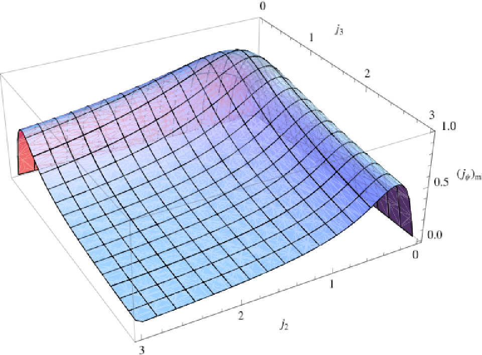
6.6 Predictions for extremal black rings

We now discuss a few features of extremal black rings that our analysis reveals. We have already mentioned that higher dimensional extremal rings can stay balanced with arbitrarily small angular momentum in the plane of the ring (essentially by being spun up in the transverse directions), see Fig. 8. This is in fact in line with the observation made for doubly spinning (non-extremal) rings five dimensions in [14] that increasing the transverse spin tends to reduce $\left(j_{\psi}\right)_{\textrm{min}}$ . Intuitively, this might be attributed to a spin-spin interaction of anti-podal components of the ring along the ${\bf S}^{1}$ .³⁶³⁶ 36 We thank Veronika Hubeny for emphasizing this point to us.

Entropy:

For large $j_{\psi}$ , the black rings are entropically more favourable (cf., Fig. 6) than the MP black holes. While such behaviour is expected for singly spinning rings (necessarily non-extremal), due to the ultra-spinning instability of the MP black holes [63], in the extremal context its origins are different. One heuristic reason for this is that thin rings are like hula-hoops, while ultra-spinning black holes (even extremal) are like disks; for given mass the disks tend to be thinner than rings and hence have smaller area [19]. Of course, we are far from Newtonian physics in this strong gravity regime of extremal black holes, but the intuitive argument serves to illustrate the essential distinction between the objects.

From Fig. 6 it is clear that the black ring area is monotonically decreasing with $j_{\psi}$ for the special case of all the transverse angular momenta being equal, unlike the MP black hole where the area is maximized at the symmetric point ( $j_{\psi}=j$ ). This is because the ring picks out a preferred direction and so the area has no characteristic feature as a function of $j_{\psi}$ . On the contrary, the absence preferred choice for MP black holes results in an asymmetric behaviour of $a_{H}(j_{\psi})$ , with a characteristic maximum. This monotonicity property for the rings is lost when we consider generic rotations in the transverse ${\bf S}^{2n}$ .

Membrane limit:

In § 3.3 we showed that the extremal MP black holes have an ultra-spinning limit following [63]; this limit appears to be more subtle for extremal black rings. To see this recall that above we demonstrated that the membrane limit commutes with the near-horizon limit for MP black holes. Now consider taking the limit in the near-horizon of an extremal black string with horizon topology ${\bf S}^{1}\times{\bf S}^{2n}$ in $D$ spacetime dimensions. We expect to obtain a black brane with horizon topology ${\bf S}^{1}\times{\bf S}^{2n-2p}\times{\bf R}^{2p}$ by the arguments of § 3.3. Ignoring the flat space factors thus generated (arising from the ${\bf R}^{2}$ s where we sent $a_{i}\to\infty$ ), we have a black string in some $D-2p$ dimensions. This string is however tensile – the pressurelessness condition (6.1) being dimension dependent, leads to differing values of the boost for the string and the membrane (in the former case we have the boost as in (6.1), while in the latter the boost would have to be $\sinh^{2}\beta=\frac{1}{2\,n-2\,p-1}$ ). So assuming that a potential membrane limit commutes with the near-horizon limits for the extremal black rings, we are led to a contradiction. On the other hand, inspection of the phase diagram Fig. 7 suggests that as one of the $j_{i}$ gets large, the ring ‘behaves’ like a lower dimensional ring. However, upon closer inspection, it appears that in addition to taking the $j_{i}\to\infty$ we need to rescale $j_{\psi}$ by a finite amount to precisely recover the lower dimensional ring’s extremal locus. This is consistent with the differing values of boost described above. Putting these things together suggests that there is no simple analog of the membrane limit of MP black holes for the black rings.

7 Discussion

The main focus of the present paper has been an exploration of vacuum extremal black holes in dimensions greater than five. As motivated in § 1 the restriction to extremal solutions is non-trivial and as we have discussed there is a rich moduli space of such solutions even in vacuum gravity. Apart from examining aspects of known examples of extremal black objects based on the MP black holes, we have also obtained predictions of certain properties of hitherto unknown extremal black ring solutions.

On the mathematical side, we have shown that vacuum solutions with degenerate horizons have an enhanced near-horizon AdS₂ isometry assuming the rotational symmetry of the solution enhances such that spatial sections of the horizon are cohomogeneity-1. From the known solutions to date, MP black holes (and strings) with equal angular momenta in even dimensions and all but one equal angular momenta in odd dimensions fall into this class of geometries. It is natural to expect that this symmetry enhancement extends to situations where the spatial sections of the horizon have less symmetry given the fact that we proved this was the case for the generic extremal MP black holes with unequal angular momenta. However, proving the general statement requires new techniques beyond those developed in [42] which we exploited. The primary complication is that the method used is well adapted to cohomogeneity-1 metrics on the horizon; higher cohomogeneity metrics occurring in the generic case are troublesome due to absence of well-adapted coordinates for the analysis. Nevertheless, given that there are high cohomogeneity metrics displaying the enhanced symmetry, it would be interesting to see if the Theorem proved in § 2.2 can be generalized.

We have also presented explicit examples of vacuum near-horizon geometries with horizon topology ${\bf S}^{D-2}$ and ${\bf S}^{1}\times{\bf S}^{D-3}$ . Of course, in higher than five dimensions one might expect other topologies. Although we have concentrated on black rings, it would be very interesting to find solutions with even more exotic horizon topology.³⁷³⁷ 37 Of course one can trivially construct vacuum near-horizon geometries by taking the direct product of ${\bf R}^{1,1}$ with a Ricci flat metric on ${\cal H}$ , $ds_{NH}^{2}=dv\,dr+ds^{2}({\cal H})$ . While this gives examples with non-trivial horizon topology they are in a sense trivial and we do not expect them to correspond to near-horizon limits of asymptotically flat black holes. It is the non-trivial examples which take the form of fibrations over AdS₂ which we are interested in.

Given the near-horizon geometry alone, an important question is how much of the physical characteristics of the solution, such as the conserved charges etc., can be determined. We have argued that while it possible using Komar integrals to capture certain angular momenta, the near-horizon metric does not capture the mass of the black object or the angular velocities (both of which depend on the asymptotic stationary frame). More generally, as discussed at end of § 2.4, a given near-horizon geometry might not always be extended to a full solution with prescribed asymptotics. Understanding the constraints on when this can be done is an interesting open question.

The new physical result in the paper is the prediction of the phase structure for extremal black rings in higher dimensions. As we have emphasized, higher dimensional black holes/rings are not easily amenable to analytic treatment owing to the lack of solution generating techniques. Given this, our strategy has been to exploit the mathematical result above, combined with certain plausible physical assumptions, to construct the phase diagram for black rings.

The logical argument for our construction of extremal black rings can be summarized as follows: given the near-horizon symmetry enhancement for degenerate horizons, extremal black rings should have a near-horizon that has three main characteristics (i) AdS₂ isometry, (ii) ring topology, and (iii) correct rotational symmetry, i.e., must be a subgroup of $SO(D-1)$ . We already know of a solution in odd spacetime dimensions with these characteristics – the near-horizon geometry of the extremal MP black string. The MP black string is not asymptotically flat, but heuristically, can be made so if the string is tensionless, by bending it. The tensionlessness condition fixes the boost parameter of the string to a numerical (dimension dependent) constant, which is independent of the transverse rotation. Our main claim is that the black string near-horizon geometry at this particular value of the boost parameter is isometric to the near-horizon geometry of an extremal black ring. The rest of the analysis is then aimed at determining the physical parameters of the black ring. We have argued that the conserved quantities of the extremal ring are the same as those for the corresponding black string.

We infer the angular momenta in the transverse sphere of the ring using the Komar integrals – these are therefore the same as the corresponding values of the MP black string. We assume the mass of the asymptotically flat black ring receives no corrections relative to the MP black string. The remaining physical parameter, the angular momentum in the plane of the ring we also argue agrees with the string. Deducing this involves realizing that the only admissible correction to the string’s angular momentum occurs at leading order in $1/\ell$ (recall that $\ell$ size of the circle wrapped by the string) and showing that such corrections do not arise in $D>5$ . This then completes the determination of the physical parameters. Finally, we put bounds on the physical parameters by requiring that black ring extremal locus is unbounded above and bounded below by the extremal locus of the MP black holes. This requirement implies uniqueness is not violated, but this is not demanded by any known theorem. Curiously, uniqueness is satisfied by the known extremal black objects in five dimensions. It would be very interesting to understand the origin of this uniqueness and explore its consequences further.

Of course, a generic feature of higher dimensional non-extremal black holes is violation of uniqueness.³⁸³⁸ 38 In the context of generalized Weyl solutions, [61] it is shown that the rod-structure of a solution together with its conserved charges fully specify the solution. Therefore, from this point of view, it seems remarkable that uniqueness is restored for extremal black holes in five dimensions. Curiously, note that the extremal doubly spinning rings do come arbitrarily close to violating uniqueness [14]. It is interesting to observe that based on our proposal, if any $c_{i}\neq 0$ (in (6.5)) it seems one cannot get extremal rings arbitrarily close to MP black holes. It is thus tempting to speculate that this suggests all $c_{i}=0$ (consistent with our final proposal), so that extremal higher dimensional rings can come arbitrarily close to violating uniqueness as in five dimensions.

Our analysis throws up some interesting features of five dimensional solutions which do not seem to be shared by their higher dimensional counterparts. Apart from the fact that extremal rings in five dimensions have slightly different characteristics (in terms of the mixing of the ring and the transverse directions), there is a curious fact about the entropy of five dimensional black objects. The area formula for extremal five dimensional MP or doubly spinning black rings takes an extremely simple form. For example, for the extremal black ring solution of [9] one has

{\cal A}_{H}=8\pi\,J_{\phi}\ .

(7.1)

The simplicity of this and analogous expressions for four and five dimensional black holes have been used to motivate a microscopic counting of the entropy of these objects [44, 45, 46, 47, 48]. These results rely on locally supersymmetric D-brane intersections (with supersymmetry being globally broken due to different supercharges being preserved at different intersections). It is well known that in dimensions greater than five there are no localized supersymmetric black holes. Further, the known extremal solutions in vacuum gravity have complicated area formulae. For example for the 6d extremal MP one has

{\cal A}_{H}=8\pi\sqrt{\sqrt{\frac{(J_{1}^{2}+J_{2}^{2})^{2}}{36}+\frac{J_{1}^{2}J_{2}^{2}}{3}}-\frac{J_{1}^{2}+J_{2}^{2}}{6}}.

(7.2)

This seems suggestive that the mechanism for micro-state counting of black holes in four and five dimensions is a happy accident of local supersymmetry, while higher dimensional extremal solutions are intrinsically more complex.

Although the focus of this paper has been on asymptotically flat vacuum black holes let us comment on AdS black holes, as some of the techniques used in this paper can easily accommodate a cosmological constant. For example, the theorem we proved on symmetry enhancement in the near-horizon limit applies equally to AdS vacuum gravity. Our discussion of extremal black holes has relied heavily on the use of Gaussian null coordinates and the ‘double-scaling’ limit which defines the near-horizon geometry (2.3). Indeed such coordinates have been used previously in the context of supersymmetric AdS₅ black holes. In particular, under some assumptions, supersymmetric AdS₅ black rings were ruled out. This was deduced from a classification of all possible near-horizon geometries of supersymmetric AdS₅ black holes with $R\times U(1)^{2}$ symmetry [38, 39].

More recently, again in the AdS/CFT context, a map relating gravitational solutions in asymptotically AdS spacetimes to solutions of conformal fluid dynamics has been constructed in a long-wavelength approximation [70, 71, 72]. The discussion so far has been for uncharged fluids just carrying energy-momentum corresponding to AdS vacuum gravity. Note that extremal solutions in pure AdS gravity cannot be supersymmetric. However, the techniques used in this paper, which rely only on extremality, could be applied to the study of “extremal” fluids. For instance, it would be interesting to exploit the Gaussian null coordinates to analyze the entropy current for such degenerate horizons, generalizing the recent analysis of [73]. It would also be interesting to develop techniques to analyze the behaviour of extremal fluids in confining gauge theories as discussed in [74, 75]. The latter analysis predicts a phase diagram for black holes and rings in AdS spacetimes using the dual field theory; this could provide an interesting test for the phase diagram proposed in this paper.

Acknowledgements

It is a great pleasure to thank Henriette Elvang, Roberto Emparan, Harvey Reall, Simon Ross and especially Veronika Hubeny for very fruitful discussions on aspects of black holes in higher dimensions. PF, JL and MR are supported by an STFC Rolling grant, while HKK is supported by a STFC postdoctoral fellowship.

Appendix A Calculating near-horizon limits

In this appendix we describe how to construct the near-horizon geometries for the MP black holes and strings given in § 2.3.1 and § 2.3.2, following the approach developed in [42]. The starting point for any of these calculations are the MP solutions which, in Boyer-Lindquist type coordinates, are:

ds^{2}=-dt^{2}+\sum_{i=1}^{n}(r^{2}+a_{i}^{2})\,(d\mu_{i}^{2}+\mu_{i}^{2}\,d\phi_{i}^{2})+\frac{\mu\,r^{2}}{\Pi\,F}\,\left(dt-\sum_{i=1}^{n}a_{i}\,\mu_{i}^{2}\,d\phi_{i}\right)^{2}+\frac{\Pi\,F}{\Pi-\mu\,r^{2}}\,dr^{2}

(A.1)

in $2n+1$ dimensions and

ds^{2}=-dt^{2}+r^{2}\,d\alpha^{2}+\sum_{i=1}^{n}(r^{2}+a_{i}^{2})(d\mu_{i}^{2}+\mu_{i}^{2}\,d\phi_{i}^{2})+\frac{\mu\,r}{\Pi\,F}\left(dt-\sum_{i=1}^{n}a_{i}\,\mu_{i}^{2}\,d\phi_{i}\right)^{2}+\frac{\Pi\,F}{\Pi-\mu\,r}\,dr^{2}

(A.2)

in $2n+2$ dimensions, where

F=1-\sum_{i=1}^{n}\,\frac{a_{i}^{2}\,\mu_{i}^{2}}{r^{2}+a_{i}^{2}}

(A.3)

and the rest of the functions and coordinates are defined as in the main text³⁹³⁹ 39 We have taken $a_{i}\to-a_{i}$ relative to the original MP metric in [18]. Without loss of generality we will assume our $a_{i}>0$ .. We are also interested in the MP black strings in $D=2n+3$ . These are constructed by taking the $2n+2$ dimensional MP metric (A.2) adding $dz^{2}$ and boosting $(t,z)\to(c_{\beta}t-s_{\beta}z\,,-s_{\beta}t+c_{\beta}z)$ where $c_{\beta}\equiv\cosh\beta$ and $s_{\beta}\equiv\sinh\beta$ .⁴⁰⁴⁰ 40 Note this is equivalent to changing coordinates to $(t^{\prime},z^{\prime})=(c_{\beta}t+s_{\beta}z\,,s_{\beta}t+c_{\beta}z)$ and then subsequently dropping the “primed”. The explicit metric for this thus reads

	$\displaystyle ds^{2}$	$\displaystyle=$	$\displaystyle-dt^{2}+dz^{2}+r^{2}\,d\alpha^{2}+\sum_{i=1}^{n}(r^{2}+a_{i}^{2})(d\mu_{i}^{2}+\mu_{i}^{2}\,d\phi_{i}^{2})$		(A.4)
			$\displaystyle+\frac{\mu\,r}{\Pi\,F}\left(c_{\beta}dt-s_{\beta}dz-\sum_{i=1}^{n}a_{i}\,\mu_{i}^{2}\,d\phi_{i}\right)^{2}+\frac{\Pi\,F}{\Pi-\mu\,r}\,dr^{2}\,.$		(A.4)

In fact it is convenient to illustrate the method of computing a near-horizon limit for a more general class of “black-hole like” metrics. This generalizes the discussion in [42]. Consider solutions of the form

	$\displaystyle ds^{2}$	$\displaystyle=$	$\displaystyle g_{tt}(R,\rho)\,dt^{2}+2\,g_{ti}(R,\rho)\,dt\,d\Phi^{i}+g_{RR}(R,\rho)\,dR^{2}$		(A.5)
			$\displaystyle\qquad+g_{pq}(R,\rho)\,d\rho^{p}\,d\rho^{q}+g_{ij}(R,\rho)\,d\Phi^{i}\,d\Phi^{j},$		(A.5)

where $p,q=1,\cdots m$ and $i,j=1,\cdots,n$ .⁴¹⁴¹ 41 Of course the integer $m$ is related to $n$ in the solutions we are dealing with but we will leave it free..The $\rho^{p}$ coordinates are a set of “polar” angles and the $\Phi^{i}$ are a set of azimuthal angles. Here $R$ is a radial coordinate and the event horizon is located at $R=0$ . We emphasize that all known black hole solutions (in any dimension), including black rings, can be written in the above form. By shifting the $\Phi^{i}$ by constant multiples of $t$ , we may always choose a co-rotating frame in which the Killing vector $\partial_{t}$ is null on the horizon, which we assume henceforth. For all known extremal black hole solutions it is the case that

g_{tt}=f_{t}(\rho)\,R^{2}+{\cal O}\left(R^{3}\right),\qquad g_{ti}=f_{i}(\rho)\,R+{\cal O}\left(R^{2}\right),\qquad g_{RR}=f_{R}(\rho)\,R^{-2}+{\cal O}\left(R^{-1}\right)

(A.6)

for functions $f_{\mu}$ that are determined from the given solution. To construct the near-horizon limit, we proceed by introducing coordinates valid on the horizon, $(v,r,\phi^{i})$ via

R=r,\qquad dt=dv+\left(\frac{a_{0}}{r^{2}}+\frac{a_{1}}{r}\right)dr\ ,\qquad d\Phi^{i}=d\phi^{i}+\frac{b_{0}^{i}}{r}\,dr\ .

(A.7)

The constants $a_{0},a_{1},b_{0}$ are fixed by requiring the metric and its inverse be analytic at the horizon $r=0$ . Now take the near-horizon limit defined by $v\to v/\epsilon,r\to\epsilon r$ with $\epsilon\to 0$ . Referring to the metric that results after taking the limit as $\hat{g}_{\mu\nu}$ , we easily obtain the following components, as they are not affected by the transformation (A.7):

\hat{g}_{vv}=f_{t}(\rho)\,r^{2},\qquad\hat{g}_{pq}=g_{pq}(0,\rho),\qquad\hat{g}_{vi}=f_{i}(\rho)\,r,\qquad\hat{g}_{ij}=g_{ij}(0,\rho).

(A.8)

Now define $k_{i}=f_{i}(\rho)$ . Elimination of the divergent $1/r$ terms in $g_{ri}$ requires

b_{0}^{i}=-a_{0}\,\gamma^{ij}(\rho)\,k_{i}=-a_{0}\,k^{i}.

(A.9)

Consistency obviously requires that the $k^{i}$ be constants. This is certainly true for the examples we are dealing with and ultimately follows from the fact that we are dealing with solutions to the field equations. Next, it is straightforward to check that, after the taking the near-horizon limit,

\Gamma\equiv\hat{g}_{vr}=a_{0}f_{t}(\rho)+b_{0}^{i}k_{i}=a_{0}(f_{t}(\rho)-k^{i}k_{i}),

(A.10)

and hence now we need only $a_{0}$ to determine the full near-horizon metric. We now turn to $g_{rr}$ . Eliminating the $1/r^{2}$ term yields the condition

a_{0}^{2}=\frac{f_{R}(\rho)}{k^{i}k_{i}-f_{t}(\rho)}.

(A.11)

This equation is only consistent if the RHS is a constant and further, since $f_{R}(\rho)>0$ a second consistency condition is that $k^{i}k_{i}-f_{t}>0$ ; again, these consistency requirements are met for the solutions we are dealing with. We could now determine $a_{1}$ by removing the $1/r$ divergence in $g_{rr}$ . However, note that $dr^{2}/r$ vanishes in the near-horizon limit, and hence to construct the near-horizon geometry we do not need $a_{1}$ . Finally, observe that we may write $\hat{g}_{vv}=f_{t}(\rho)r^{2}=(a_{0}^{-1}\Gamma+k^{i}k_{i})r^{2}$ . Putting this all together, we have the following cohomogeneity- $m$ near-horizon geometry:

ds^{2}=\Gamma(\rho)[a_{0}^{-1}r^{2}dv^{2}+2dvdr]+\hat{g}_{pq}(\rho)d\rho^{p}d\rho^{q}+\gamma_{ij}(\rho)(d\phi^{i}+rk^{i}dv)(d\phi^{j}+rk^{j}dv).

(A.12)

We choose signs such that $\Gamma>0$ , so we are dealing with a future horizon. This implies $a_{0}<0$ . In this form, it is clear that the near-horizon geometry has an $SO(2,1)\times U(1)^{n}$ isometry.

References

[1] R. Emparan and H. S. Reall, “Generalized Weyl solutions,” Phys. Rev. D65 (2002) 084025, hep-th/0110258.
[2] R. Emparan and H. S. Reall, “A rotating black ring in five dimensions,” Phys. Rev. Lett. 88 (2002) 101101, hep-th/0110260.
[3] R. Emparan and H. S. Reall, “Black rings,” Class. Quant. Grav. 23 (2006) R169, hep-th/0608012.
[4] V. A. Belinsky and V. E. Zakharov, “Integration of the Einstein Equations by the Inverse Scattering Problem Technique and the Calculation of the Exact Soliton Solutions,” Sov. Phys. JETP 48 (1978) 985–994.
[5] V. A. Belinsky and V. E. Sakharov, “Stationary Gravitational Solitons with Axial Symmetry,” Sov. Phys. JETP 50 (1979) 1–9.
[6] T. Mishima and H. Iguchi, “New axisymmetric stationary solutions of five-dimensional vacuum Einstein equations with asymptotic flatness,” Phys. Rev. D73 (2006) 044030, hep-th/0504018.
[7] P. Figueras, “A black ring with a rotating 2-sphere,” JHEP 07 (2005) 039, hep-th/0505244.
[8] S. Tomizawa, Y. Morisawa, and Y. Yasui, “Vacuum solutions of five dimensional Einstein equations generated by inverse scattering method,” Phys. Rev. D73 (2006) 064009, hep-th/0512252.
[9] A. A. Pomeransky and R. A. Sen’kov, “Black ring with two angular momenta,” hep-th/0612005.
[10] H. Elvang and P. Figueras, “Black Saturn,” JHEP 05 (2007) 050, hep-th/0701035.
[11] H. Iguchi and T. Mishima, “Black di-ring and infinite nonuniqueness,” Phys. Rev. D75 (2007) 064018, hep-th/0701043.
[12] J. Evslin and C. Krishnan, “The Black Di-Ring: An Inverse Scattering Construction,” arXiv:0706.1231 [hep-th].
[13] K. Izumi, “Orthogonal black di-ring solution,” arXiv:0712.0902 [hep-th].
[14] H. Elvang and M. J. Rodriguez, “Bicycling Black Rings,” 0712.2425.
[15] R. Emparan and H. S. Reall, “Black Holes in Higher Dimensions,” 0801.3471.
[16] N. A. Obers, “Black Holes in Higher-Dimensional Gravity,” 0802.0519.
[17] T. Harmark, “Stationary and axisymmetric solutions of higher- dimensional general relativity,” Phys. Rev. D70 (2004) 124002, hep-th/0408141.
[18] R. C. Myers and M. J. Perry, “Black Holes in Higher Dimensional Space-Times,” Ann. Phys. 172 (1986) 304.
[19] R. Emparan, T. Harmark, V. Niarchos, N. A. Obers, and M. J. Rodriguez, “The Phase Structure of Higher-Dimensional Black Rings and Black Holes,” JHEP 10 (2007) 110, 0708.2181.
[20] J. L. Hovdebo and R. C. Myers, “Black rings, boosted strings and Gregory-Laflamme,” Phys. Rev. D73 (2006) 084013, hep-th/0601079.
[21] H. Elvang, R. Emparan, and A. Virmani, “Dynamics and stability of black rings,” JHEP 12 (2006) 074, hep-th/0608076.
[22] J. P. Gauntlett, J. B. Gutowski, C. M. Hull, S. Pakis, and H. S. Reall, “All supersymmetric solutions of minimal supergravity in five dimensions,” Class. Quant. Grav. 20 (2003) 4587–4634, hep-th/0209114.
[23] H. S. Reall, “Higher dimensional black holes and supersymmetry,” Phys. Rev. D68 (2003) 024024, hep-th/0211290.
[24] J. P. Gauntlett and J. B. Gutowski, “All supersymmetric solutions of minimal gauged supergravity in five dimensions,” Phys. Rev. D68 (2003) 105009, hep-th/0304064.
[25] J. B. Gutowski and H. S. Reall, “Supersymmetric AdS(5) black holes,” JHEP 02 (2004) 006, hep-th/0401042.
[26] J. B. Gutowski and H. S. Reall, “General supersymmetric AdS(5) black holes,” JHEP 04 (2004) 048, hep-th/0401129.
[27] J. B. Gutowski, “Uniqueness of five-dimensional supersymmetric black holes,” JHEP 08 (2004) 049, hep-th/0404079.
[28] D. Gaiotto, A. Strominger, and X. Yin, “New connections between 4D and 5D black holes,” JHEP 02 (2006) 024, hep-th/0503217.
[29] H. Elvang, R. Emparan, D. Mateos, and H. S. Reall, “A supersymmetric black ring,” Phys. Rev. Lett. 93 (2004) 211302, hep-th/0407065.
[30] D. Gaiotto, A. Strominger, and X. Yin, “5D black rings and 4D black holes,” JHEP 02 (2006) 023, hep-th/0504126.
[31] I. Bena and N. P. Warner, “One ring to rule them all … and in the darkness bind them?,” Adv. Theor. Math. Phys. 9 (2005) 667–701, hep-th/0408106.
[32] J. P. Gauntlett and J. B. Gutowski, “Concentric black rings,” Phys. Rev. D71 (2005) 025013, hep-th/0408010.
[33] H. Elvang, R. Emparan, D. Mateos, and H. S. Reall, “Supersymmetric black rings and three-charge supertubes,” Phys. Rev. D71 (2005) 024033, hep-th/0408120.
[34] J. P. Gauntlett and J. B. Gutowski, “General concentric black rings,” Phys. Rev. D71 (2005) 045002, hep-th/0408122.
[35] H. Elvang, R. Emparan, D. Mateos, and H. S. Reall, “Supersymmetric 4D rotating black holes from 5D black rings,” JHEP 08 (2005) 042, hep-th/0504125.
[36] I. Bena, P. Kraus, and N. P. Warner, “Black rings in Taub-NUT,” Phys. Rev. D72 (2005) 084019, hep-th/0504142.
[37] H. K. Kunduri, J. Lucietti, and H. S. Reall, “Supersymmetric multi-charge AdS(5) black holes,” JHEP 04 (2006) 036, hep-th/0601156.
[38] H. K. Kunduri, J. Lucietti, and H. S. Reall, “Do supersymmetric anti-de Sitter black rings exist?,” JHEP 02 (2007) 026, hep-th/0611351.
[39] H. K. Kunduri and J. Lucietti, “Near-horizon geometries of supersymmetric AdS(5) black holes,” JHEP 12 (2007) 015, arXiv:0708.3695 [hep-th].
[40] A. Sen, “Black Hole Entropy Function, Attractors and Precision Counting of Microstates,” arXiv:0708.1270 [hep-th].
[41] J. M. Bardeen and G. T. Horowitz, “The extreme Kerr throat geometry: A vacuum analog of AdS(2) x S(2),” Phys. Rev. D60 (1999) 104030, hep-th/9905099.
[42] H. K. Kunduri, J. Lucietti, and H. S. Reall, “Near-horizon symmetries of extremal black holes,” Class. Quant. Grav. 24 (2007) 4169–4190, arXiv:0705.4214 [hep-th].
[43] R. Emparan, “Rotating circular strings, and infinite non-uniqueness of black rings,” JHEP 03 (2004) 064, hep-th/0402149.
[44] R. Emparan and G. T. Horowitz, “Microstates of a neutral black hole in M theory,” Phys. Rev. Lett. 97 (2006) 141601, hep-th/0607023.
[45] R. Emparan and A. Maccarrone, “Statistical description of rotating Kaluza-Klein black holes,” Phys. Rev. D75 (2007) 084006, hep-th/0701150.
[46] G. T. Horowitz and M. M. Roberts, “Counting the Microstates of a Kerr Black Hole,” Phys. Rev. Lett. 99 (2007) 221601, arXiv:0708.1346 [hep-th].
[47] H. S. Reall, “Counting the microstates of a vacuum black ring,” arXiv:0712.3226 [hep-th].
[48] R. Emparan, “Exact Microscopic Entropy of Non-Supersymmetric Extremal Black Rings,” arXiv:0803.1801 [hep-th].
[49] A. Dabholkar, A. Sen, and S. P. Trivedi, “Black hole microstates and attractor without supersymmetry,” JHEP 01 (2007) 096, hep-th/0611143.
[50] D. Astefanesei, K. Goldstein and S. Mahapatra, “Moduli and (un)attractor black hole thermodynamics,” hep-th/0611140.
[51] D. Astefanesei, K. Goldstein, R. P. Jena, A. Sen, and S. P. Trivedi, “Rotating attractors,” JHEP 10 (2006) 058, hep-th/0606244.
[52] D. Astefanesei and H. Yavartanoo, “Stationary black holes and attractor mechanism,” Nucl. Phys. B 794 (2008) 13, arXiv:0706.1847 [hep-th].
[53] N. V. Suryanarayana and M. C. Wapler, “Charges from Attractors,” Class. Quant. Grav. 24 (2007) 5047–5072, arXiv:0704.0955 [hep-th].
[54] K. Hanaki, K. Ohashi, and Y. Tachikawa, “Comments on charges and near-horizon data of black rings,” JHEP 12 (2007) 057, arXiv:0704.1819 [hep-th].
[55] J. Isenberg and V. Moncrief, “Symmetries of Cosmological Cauchy Horizons,” Commun. Math. Phys. 89 (1983) 387–413.
[56] S. Hollands, A. Ishibashi, and R. M. Wald, “A higher dimensional stationary rotating black hole must be axisymmetric,” Commun. Math. Phys. 271 (2007) 699–722, gr-qc/0605106.
[57] P. T. Chrusciel, H. S. Reall, and P. Tod, “On non-existence of static vacuum black holes with degenerate components of the event horizon,” Class. Quant. Grav. 23 (2006) 549–554, gr-qc/0512041.
[58] A. Sen, “Black hole entropy function and the attractor mechanism in higher derivative gravity,” JHEP 09 (2005) 038, hep-th/0506177.
[59] J. M. Bardeen, B. Carter, and S. W. Hawking, “The Four laws of black hole mechanics,” Commun. Math. Phys. 31 (1973) 161–170.
[60] H. Elvang, R. Emparan, and P. Figueras, “Phases of Five-Dimensional Black Holes,” JHEP 05 (2007) 056, hep-th/0702111.
[61] S. Hollands and S. Yazadjiev, “A Uniqueness theorem for 5-dimensional Einstein-Maxwell black holes,” arXiv:0711.1722 [gr-qc].
[62] B. Kleihaus, J. Kunz, and F. Navarro-Lerida, “Rotating Black Holes in Higher Dimensions,” arXiv:0710.2291 [hep-th].
[63] R. Emparan and R. C. Myers, “Instability of ultra-spinning black holes,” JHEP 09 (2003) 025, hep-th/0308056.
[64] R. C. Myers, “Stress tensors and Casimir energies in the AdS/CFT correspondence,” Phys. Rev. D60 (1999) 046002, hep-th/9903203.
[65] P. K. Townsend and M. Zamaklar, “The first law of black brane mechanics,” Class. Quant. Grav. 18 (2001) 5269–5286, hep-th/0107228.
[66] T. Harmark and N. A. Obers, “General definition of gravitational tension,” JHEP 05 (2004) 043, hep-th/0403103.
[67] D. Kastor, S. Ray, and J. Traschen, “The First Law for Boosted Kaluza-Klein Black Holes,” JHEP 06 (2007) 026, arXiv:0704.0729 [hep-th].
[68] H. Elvang and R. Emparan, “Black rings, supertubes, and a stringy resolution of black hole non-uniqueness,” JHEP 11 (2003) 035, hep-th/0310008.
[69] W. Israel, “Source of the Kerr Metric,” Phys. Rev. D2 (1970), no. 4, 641–646.
[70] S. Bhattacharyya, S. Lahiri, R. Loganayagam, and S. Minwalla, “Large rotating AdS black holes from fluid mechanics,” arXiv:0708.1770 [hep-th].
[71] S. Bhattacharyya, V. E. Hubeny, S. Minwalla, and M. Rangamani, “Nonlinear Fluid Dynamics from Gravity,” arXiv:0712.2456 [hep-th].
[72] M. Van Raamsdonk, “Black Hole Dynamics From Atmospheric Science,” arXiv:0802.3224 [hep-th].
[73] S. Bhattacharyya, V. E. Hubeny, R. Loganayagam, G. Mandal, S. Minwalla, T. Morita, M. Rangamani, and H. S. Reall, “Local fluid dynamical entropy from gravity,” arXiv:0803.2526 [hep-th].
[74] O. Aharony, S. Minwalla, and T. Wiseman, “Plasma-balls in large N gauge theories and localized black holes,” Class. Quant. Grav. 23 (2006) 2171–2210, hep-th/0507219.
[75] S. Lahiri and S. Minwalla, “Plasmarings as dual black rings,” arXiv:0705.3404 [hep-th].

Extremal vacuum black holes in higher dimensions

1 Introduction

2 Near-horizon geometries

2.1 Gaussian null coordinates and the near-horizon limit

2.2 Symmetry enhancement in the near-horizon limit: S​O​(2,1)SO(2,1)

Theorem:

Proof:

Remarks:

2.3 Examples of near-horizon metrics

2.3.1 Spherical topology horizons

2.3.2 Black ring topology horizons

2.4 What physical data can be extracted from a near-horizon geometry?

Angular momenta:

Mass:

3 Extremal MP black holes

3.1 Parameterization of MP black holes

3.2 The extremal locus

3.3 Membrane limits of MP black holes

4 Extremal MP black strings

5 Extremal black rings in five dimensions

6 Extremal Black rings in higher dimensions

6.1 Extremal black rings as black strings

Symmetries:

Infinite radius limit:

Near-horizon limit:

6.2 Conserved charges of extremal black rings

Summary:

6.3 Determining angular momentum in the plane of the ring

6.4 Bounds on black ring parameters and uniqueness

6.5 Phase diagrams of extremal black rings

6.6 Predictions for extremal black rings

Entropy:

Membrane limit:

7 Discussion

Acknowledgements

Appendix A Calculating near-horizon limits

References

Extremal vacuum black holes in
higher dimensions

2.2 Symmetry enhancement in the near-horizon limit: $SO(2,1)$