,
Driven particle in a cloud of mobile impurities
Abstract
The dynamics of a test particle interacting with diffusing impurities in one dimension is investigated analytically and numerically. In the absence of an applied external force, the dynamics of the particle can be characterized by a distribution of monotonic excursions , which scales as a power law with an exponent . When the particle is driven at a slow constant velocity, there is again a power law distribution for the monotonic changes of the force , which is characterized by a similar exponent . These results can be understood from the theory of random walks.
pacs
05.40.-a, 66.30.J-, 61.72.Yx1 Introduction
The interaction of driven particles, flexible lines and membranes etc. with disorder is an important topic in condensed matter physics [1, 2, 3]. Usually, this disorder is taken to be quenched, or frozen, such that its properties do not change within the relevant time scales. However, under certain conditions, this changes as in the case of the diffusion of solute atoms in metallic alloys [4, 5] or oxygen vacancies in superconductors [6]. The mobile impurities play an important role in the dynamics of such systems, as evidenced for example by the Portevin-Le Chatelier (PLC) effect in solid solutions [7]. There, within a certain range of temperatures and applied strain rates, the dynamic interaction of lattice dislocations and diffusing solute atoms result in phenomena such as negative strain rate sensitivity of the flow stress, giving rise to macroscopic serrations in the stress strain curve and strain localization in the form of bands of activity of various types [8, 9, 10].
Here, we consider the simple test problem of a single particle interacting with a cloud of diffusing impurities, with the dynamics constrained in one dimension (a line). We restrict ourselves to the region of the parameter space in which the impurities have a vanishingly small probability to escape from the vicinity of the particle. Despite its apparent simplicity, such a system exhibits rich dynamics, but at the same time has features that make the problem analytically tractable. In the absence of external forces, we consider the statistics of monotonic excursions of the particle, i.e. the distances the particle moves to a particular direction (here “left” or “right” along the one-dimensional line) without changing direction, see also figure 1. We find that these obey power law distributions with the exponent . The same is true for the monotonic changes of the external force when the particle is driven with a slow constant velocity. This paper is organized as follows: In the next section, we consider the interaction of a particle with a single mobile impurity, in the absence of external forces. Then we generalize this to the case with more impurity particles. In section 3, the effect of external drive is studied. Finally, section 4 finishes the paper with conclusions.
2 A particle interacting with mobile impurities
2.1 Single impurity
As a starting point of our analysis, we consider the dynamics of a single particle interacting with one diffusing impurity particle. The equations of motion for the system are
| (1) |
where and are the positions of the particle and the impurity particle, respectively. is the interaction force between the particle and the impurity particle, defines the relative mobilities of the impurity and the particle and is Gaussian white noise with standard deviation mimicking the effect of temperature.
The dynamics of the particle can be analyzed by considering the stochastic process for the velocity . By differentiating the equation of motion of the particle with respect to time and using the equation of motion for , one obtains
| (2) |
Close to , the force can be taken to be linear in and thus the derivative of the force can be approximated by a constant, , with . With and , equation (2) can then be rewritten in the form of an Ornstein-Uhlenbeck process for ,
| (3) |
For the process , equation (3) describes Brownian motion pushed toward the origin by a linear damping term. This problem has been considered e.g. in [11], and the scaling exponents are known. In particular, the first return times to origin of have a probability distribution scaling as
| (4) |
with and the cut-off scale . Similarly, the average shape of an excursion, , scales for as , with . Then, by using the scaling relation [12], one obtains the distribution of the lengths of monotonic excursions of the particle,
| (5) |
with . The cut-off scaling can be found as follows: The cut-off of the first return time distribution of equation (3) is given by [11]. Here, both and in equation (3) depend on and . Due to the relation with , is expected to scale like
| (6) |


We check this result in numerical simulations, where we take for simplicity to be of the form , corresponding to , i.e. . We integrate the equations of motion (1) with the Euler algorithm. The strength of the thermal noise was chosen to be sufficiently weak such that the impurity cannot escape from the neighborhood of the particle. Figure 1 shows an example of the trajectories of the particle and the impurity. Figure 2 displays the distribution of for various values of . For a weak enough interaction strength A, the distributions display the expected scaling with . The cut-off is found to scale as , in agreement with our results above.
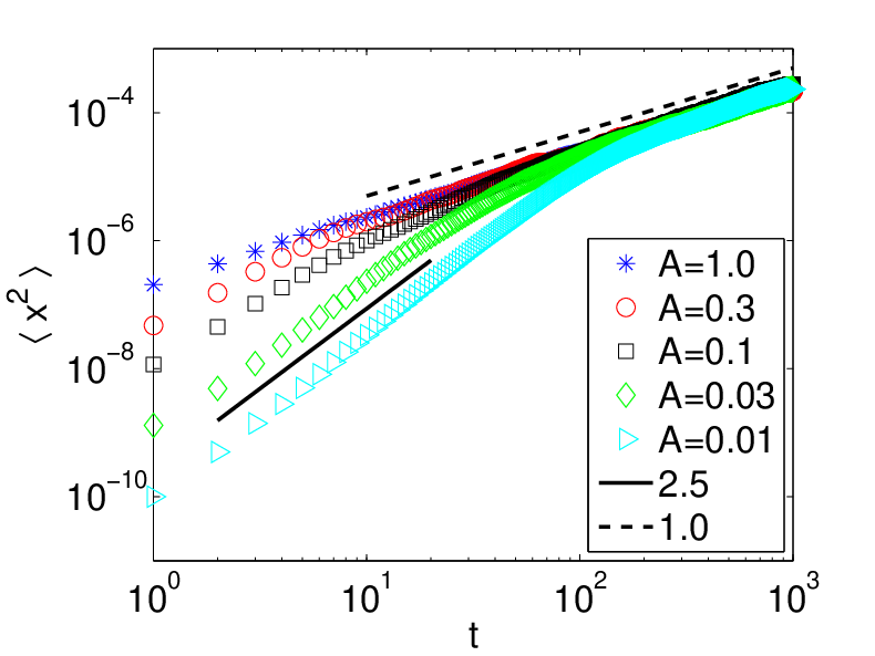
This implies that the motion of the particle is reminiscent of truncated Levy flight, with a step length distribution given by equation (5). However, the steps are not instantaneous - their durations exhibit power law scaling as well, equation (4). By interpreting these step durations as waiting times between instantaneous steps, one would obtain for early times the scaling . However, here and are not independent (due to the relation ). As the early time behavior is dominated by a single large step, one must consider instead the effect of a single step given its duration,
| (7) |
corresponding to . Due to the truncated nature of the Levy flight, one expects a cross-over to diffusive behavior with for long times. This is verified in figure 3.
2.2 Several impurities
The case of a fixed number of impurity particles is a straightforward generalization of that presented in the previous subsection. The equations of motion become
| (8) |
From these equations, with the same procedure as above, one obtains an equation of the form of equation (3) by setting and . Thus, the same scaling, i.e. is expected. One should notice, however, that the cut-off scale is getting smaller with increasing . With similar arguments as above, one finds that
| (9) |
This is verified by the numerical results presented in figure 4.

3 Constant velocity drive
Next we proceed to study the effect of a weak external force on the dynamics of the particle. In this context a constant velocity drive is perhaps the more interesting form of driving as a small constant force with does not change the dynamics from the non-driven case: equation (2) remains the same even if a constant force term is introduced in equation (1). In particular, we consider a particle driven by a force given by , where is the driving velocity and is a spring constant characterizing the response of the driving mechanism. The equations of motion read
| (10) |
In systems like this driven with a constant velocity, the interesting quantity is the statistics of the external force fluctuations. To this end, we consider the stochastic process . With a similar approach as above, one can write
| (11) | |||||
where the relation has been used. In the steady state, the last term in equation (11) has a zero mean, as one can write for the average steady state force , where is the magnitude of the average retarding force acting on the particle due to a single impurity. In the steady state the condition holds, and thus . Assuming that the fluctuations are small compared to those of the white noise term in equation (11), i.e. , equation (11) can be approximately written as
| (12) |
which is again of the same form as equation (3). Thus, the monotonic changes of the external force are expected to be distributed according to a power law , with the exponent and the cut-off scale scaling as
| (13) |
Notice that the condition implies that
| (14) |
For most of the relevant parameter values condition (14) is fulfilled, only for this is not the case.


Next we check these predictions numerically for different values of the parameters satisfying the condition (14). Figure 5 shows an example of the behaviour of the force as a function of time. After an initial transient, the system reaches a steady state in which the force fluctuates around a constant average value. In figure 6, we show the distributions of the monotonic changes of the external force in the steady state, for different values of the various parameters. Power law scaling of the distributions consistent with the exponent value is observed, with a cut-off of the distributions in agreement with equation (13). The different -values appear to be uncorrelated in time.
4 Conclusions
In this paper we have studied the dynamics of a single particle interacting with a cloud of diffusing impurities. In the absence of external forces, the problem can be mapped to Brownian motion in a potential within the harmonic approximation of the attractive particle-impurity interaction. Thus, the monotonic excursions of the particle are distributed as a power law, , with . For a particle driven with a small constant velocity (such that the particle is dragging the impurity cloud without escaping from it), the external force fluctuations follow the same dynamics, which makes it possible to derive the probability distribution for the monotonic changes of the external force scaling as , again with .
While a typical experimentally relevant scenario would correspond to either a higher dimensional object such as a flexible line or a large number of interacting particles interacting with mobile impurities, the simple setup of the present study serves as a convenient starting point for such considerations illustrating the relevant phenomena in a transparent manner. One interesting observation is that already at the level of a single particle interacting with one or more mobile impurities the dynamics has scale free features, arising from the properties of simple random walks. Physical situations in which these kind of considerations could be relevant include dislocations interacting with solute atoms, a subject that has recently attracted considerable attention [13, 14, 15]. In many of these studies, more realistic interaction forces between dislocations and solute atoms have been used, but the focus has been on different quantities such as the average velocity of the dislocation.
The most intriguing phenomena associated with the presence of diffusing impurities are the collective effects arising from the simultaneous interaction of large number of entities with each other and with mobile impurities. An example of such a system is provided by interacting dislocation ensembles interacting with diffusing solute atoms in solid solutions, giving rise to phenomena such as the Portevin-Le Chatelier effect. In the PLC effect, large numbers of dislocations synchronize their motion to form macroscopic deformation bands of various kinds. As this is widely believed to be due to the dynamic interaction of the dislocations with the diffusing solute atoms, a natural future line of research would be to study such effects by considering numerically the dynamics of a large number of interacting dislocations interacting with diffusing impurities. One further motivation for such studies could be the recent observation that purely stochastic effects can induce switching between collective motion states [16].
References
References
- [1] Nattermann T 1983 Phys. Status Solidi B 119 209
- [2] Huse D A and Henley C L 1985 Phys. Rev. Lett. 54 2708
- [3] Kardar M and Zhang Y C 1987 Phys. Rev. Lett. 58 2087
- [4] Cahn J W 1962 Acta metall. 10 789
- [5] Blavette D, Cadel E, Fraczkiewicz A, and Menand A 1999 Science 286 2317
- [6] Chudnovsky E M 1998 Europhys. Lett. 43 445
- [7] Portevin A and Le Chatelier F 1923 C. R. Acad. Sci. Paris 176 507
- [8] Ananthakrishna G, Noronha S J, Fressengeas C, and Kubin L P 1999 Phys. Rev. E 60 5455
- [9] Lebyodkin M A, Brechet Y, Estrin Y, and Kubin L P 1995 Phys. Rev. Lett. 74 4758
- [10] Hähner P, Ziegenbein A, Rizzi E, and Neuhäuser H 2002 Phys. Rev. B 65, 134109
- [11] Colaiori F, Baldassaarri A, and Castellano C 2004 Phys. Rev. E 69 041105
- [12] Lubeck S 2004 Int J. Mod. Phys. B 18 3977
- [13] Wang Y, Srolovitz D J, Rickman J M, and LeSar R 2000 Acta Mater. 48 2163
- [14] Rickman J M, LeSar R, and Srolovitz D J 2003 Acta Mater. 51 1199
- [15] Deo C S, Srolovitz D J, Cai W, and Bulatov V 2005 Phys. Rev. B 71 014106
- [16] Kolpas A, Moehlis J, and Kevrekidis I G 2007 PNAS 104 5931