Measurement of the baryonic acoustic oscillation scale in 21 cm intensity fluctuations during the reionisation era
Abstract
It has recently been suggested that the power spectrum of redshifted 21 cm fluctuations could be used to measure the scale of baryonic acoustic oscillations (BAOs) during the reionisation era. The resulting measurements are potentially as precise as those offered by the next generation of galaxy redshift surveys at lower redshift. However unlike galaxy redshift surveys, which in the linear regime are subject to a scale independent galaxy bias, the growth of ionised regions during reionisation is thought to introduce a strongly scale dependent relationship between the 21 cm and mass power spectra. We use a semi-numerical model for reionisation to assess the impact of ionised regions on the precision and accuracy with which the BAO scale could be measured using redshifted 21 cm observations. For a model in which reionisation is completed at , we find that the constraints on the BAO scale are not systematically biased at . In this scenario, and assuming the sensitivity attainable with a low-frequency array comprising 10 times the collecting area of the Murchison Widefield Array, the BAO scale could be measured to within 1.5 per cent in the range .
Keywords:
cosmology: diffuse radiation – large-scale structure of the universe1 Introduction
The imprint of baryonic acoustic oscillations (BAOs) on the mass power spectrum (PS) provides a cosmic yardstick that can be used to measure the dependence of both the angular diameter distance and Hubble parameter on redshift. The wavelength of a BAO is related to the size of the sound horizon at recombination. Its value depends on the Hubble constant, and on the dark matter and baryon densities. However, it does not depend on the amount or nature of dark energy. Thus measurements of the angular diameter distance and Hubble parameter can in turn be used to constrain the possible evolution of dark energy with cosmic time (Eisenstein et al., 1998; Eisenstein, 2002, e.g.).
Galaxy surveys have proved to be a powerful probe of the linear PS on large scales and therefore provide a means to measure the BAO scale (Blake & Glazebrook, 2003; Seo & Eisenstein, 2003; Seo & Eisenstein, 2005; Glazebrook & Blake, 2005; Hu & Haiman, 2003; Seo & Eisenstein, 2007; Angulo et al., 2008, e.g.). Indeed, analyses of the galaxy PS from the SDSS and 2dFGRS surveys have uncovered a BAO signal (Cole et al., 2005; Eisenstein et al., 2005; Percival et al., 2007; Okumura et al., 2008; Gaztanaga et al., 2008a; Gaztanaga et al., 2008b, e.g.), providing incentive for deeper all-sky galaxy surveys, using telescopes like the SKA11 1 http://www.skatelescope.org, Pan-STARRS22 2 http://pan-starrs.ifa.hawaii.edu/public and the LSST33 3 http://www.lsst.org, to measure the BAO scale and hence the dark energy equation of state more accurately.
Galaxy redshift surveys are best suited to studies of the dark energy equation of state at relatively late times () due to the difficulty of obtaining accurate redshifts for a sufficiently large number of high redshift galaxies. Although detection of the Integrated Sachs-Wolfe effect puts some constraints on the integrated role of dark energy above [see, e.g., Giannantonio et al. (2008) and references therein], we currently have very limited information about the nature of dark energy at high redshift. If dark energy behaves like a cosmological constant, then its effect on the Hubble expansion is only significant at and becomes negligible at . In this case, studies of the BAO scale at low redshift would provide the most powerful constraints. However, as the origin of dark energy is not understood we cannot presume a priori which redshift range should be studied in order to provide optimal constraints on proposed models. Probes of dark energy at higher redshifts have been suggested. These include measurements of the PS from a Ly forest survey which could potentially be used probe the evolution of dark energy through measurement of the BAO scale for redshifts as high as (McDonald & Eisenstein, 2007). Similarly, studying the temporal variation of high resolution quasar spectra may probe the evolution of dark energy through the Sandage-Loeb test in the window (Corasaniti et al., 2007). Measurements of the BAO scale in the reionisation era () are likely to be complimentary to the constraints at lower redshifts provided by these techniques.
It has recently been suggested that observations of 21 cm intensity fluctuations might provide an additional avenue to measure the mass PS (McQuinn et al., 2006; Bowman et al., 2006; Mao et al., 2008, e.g.), and that future low-frequency arrays could be used to measure the BAO scale at a range of redshifts (Wyithe et al., 2008; Chang et al., 2008; Mao & Wu, 2008). Redshifted 21 cm surveys are sensitive to neutral hydrogen regardless of whether it is part of a resolved object. As a result, at high redshifts such surveys may be more efficient in measuring the large-scale mass distribution than galaxy redshift surveys, which must identify a very large number of individual galaxies. Furthermore, spectroscopic emission line surveys have the advantage of probing a precisely defined redshift interval, which is unlikely to be true of a traditional galaxy survey (Simpson & Bridle, 2006, see).
Planned low-frequency arrays such as the Murchison Widefield Array44 4 http://www.haystack.mit.edu/ast/arrays/mwa (MWA) and LOFAR55 5 http://www.lofar.org are designed to measure the PS of 21 cm fluctuations at in order to probe the reionisation era. Wyithe et al. (2008) have argued that while the first generation of low-frequency arrays will not have sufficient sensitivity to precisely determine the BAO scale, future extensions could have the sensitivity to detect the BAO scale with promisingly small errors. Wyithe et al. (2008) assumed a semi-analytic model which predicts a scale independent value for the effective bias between the linear matter PS and the 21 cm PS. However the 21 cm bias is expected to be strongly scale dependent, especially toward the end of reionisation when many ionised bubbles percolate through the intergalactic medium (IGM), creating an excess of power on scales larger than the characteristic bubble size (Furlanetto et al., 2004, e.g.). In this paper we explore whether the scale dependence of the 21 cm bias will compromise the ability of redshifted 21 cm observations to measure the BAO scale (Mao & Wu, 2008). We begin by reviewing the expected BAO signal and 21 cm PS in Section 2. We describe the observation of the 21 cm PS, including a discussion of the noise considerations in Section 3. In Section 4 we describe our fitting procedure for recovering the BAO scale and present our error analysis, before concluding in Section 5. To calculate these errors we adopt a set of cosmological parameters similar to those derived from the third year WMAP data (Spergel et al., 2007), namely and .
2 Theoretical background
The sound speed at recombination determines the length scale of the acoustic peaks in both the cosmic microwave background (CMB) anisotropies and the linear matter PS. We refer to this length as the BAO scale. The co-moving horizon size at decoupling may be determined from knowledge of and , and an understanding of the physics governing a baryon-photon fluid (Page et al., 2003). Komatsu et al. (2008) calculate this length scale to be Mpc for the cosmological parameters extracted from the fifth year WMAP data. The corresponding angular scale is closely related to the position of the first acoustic peak in the CMB PS, which occurs at the scale of the mode which has compressed once at the time of decoupling (Page et al., 2003, see). Following decoupling the same acoustic scale is imprinted in the matter PS, albeit with a different phase. This signature is expected to be preserved on large scales where non-linear gravitational effects are small. Therefore the BAO scale may be used as a standard ruler to test the geometry of the universe and the role of dark energy.
2.1 Theoretical expectations for the redshifted 21 cm power spectrum
Neutral hydrogen radiates at 21 cm due to the hyperfine transition between the singlet and triplet ground states. Assuming a contrast between the kinetic temperature of the IGM and the CMB temperature , and efficient coupling of the spin temperature to , the 21 cm signal will mirror the underlying density of neutral hydrogen. The Ly and X-ray flux emitted by the first galaxies is expected to ensure these conditions hold during most of the reionisation era (Furlanetto, 2006, see, e.g.,). A radio interferometer is sensitive to fluctuations in the brightness temperature of neutral gas. For gas of mean cosmic density the expected temperature brightness contrast in redshifted 21 cm emission is
| (1) | |||||
where is the optical depth of the neutral gas to 21 cm radiation and is the mass-weighted neutral fraction of hydrogen in the IGM.
Allowing for fractional fluctuations in the baryonic matter density , ionised fraction , and peculiar gas velocity (where is the peculiar velocity of the gas)66 6 Variations in the local Ly- flux may also result in fluctuations in the signal through , (Barkana & Loeb, 2005b, e.g.), the spatial dependence of the brightness temperature fluctuations may be written (Mao & Wu, 2008, e.g.)
| (2) | |||||
Assuming the peculiar velocity effect is described by the linear theory result from Kaiser (1987), i.e. (note that in the high redshift limit) where denotes the angle between the line of sight and the Fourier vector , the angle dependent 21 cm power-spectrum may be written (Mao & Wu, 2008, e.g.)
| (3) | |||
, and are the linear matter power-spectrum, ionisation power-spectrum, and ionisation-density cross power-spectrum respectively. In general the 21 cm PS will display complex angle and redshift dependent structure. The difference in the angular dependence modulating the cosmological () and astrophysical () components may be able to be exploited to constrain both cosmological and astrophysical parameters (Barkana & Loeb, 2005a; Mao & Wu, 2008, e.g.). The spherically averaged 21 cm PS may be more simply related to the underlying mass PS via
| (4) |
where is the primordial linear matter PS extrapolated to calculated using CMBfast (Seljak & Zaldarriaga, 1996), and is the linear growth factor between redshift and the present. In equation (4), the prefactor is a term which is analogous to galaxy bias (but which has units of mK). However in contrast to galaxy redshift surveys, the value of can be scale dependent, even in the linear regime, as a result of the long-range, non-gravitational correlations introduced into the ionisation structure of the IGM by the formation of HII regions. Whilst peculiar velocity effects will be present, Seo & Eisenstein (2005) find that the BAO signal is preserved in the matter PS at . Furthermore, Seo et al. (2008) and Shaw & Lewis (2008) show that even the effect of non-linear redshift space distortions on the spherically averaged matter PS may be able to be corrected to high accuracy.
Equation (4) implicitly assumes that the gravitational dynamics governing the large-scale structures probed are well described by linearised fluid equations. Non-linear gravitational dynamics will be increasingly important at low redshift. However at the redshifts of interest here () non-linear evolution is unlikely to play a significant role (Crocce & Scoccimarro, 2008; Mao & Wu, 2008, see, e.g.). Mao et al. (2008) find that the cut-off in the maximum wave-number probed by redshifted 21 cm PS in the range has little affect on the constraints on cosmological parameters.
2.2 Model for the evolution of the 21 cm signal
In the early stages of reionisation when most of the hydrogen is still neutral, the bias between the linear matter PS and the 21 cm PS, , is well approximated by a constant with units of temperature. However the bias is expected to depend on scale during the process of reionisation since galaxies preferentially form in overdense regions, resulting in early formation of ionised bubbles from an overdense IGM. This effect can be modelled semi-analytically (Wyithe & Morales, 2007, e.g.), or with full numerical calculations of reionisation (McQuinn et al., 2007a; McQuinn et al., 2007b; Trac & Cen, 2007, e.g.). Recently, semi-numerical schemes have been devised which allow efficient calculation of the large-scale ionisation field (Mesinger & Furlanetto, 2007; Zahn et al., 2007; Geil & Wyithe, 2008). We use simulations computed using the method described in Geil & Wyithe (2008) to model . We refer the reader to the discussion of the semi-numerical modeling in that paper, and to the discussion of the underlying semi-analytic model for the reionisation of the IGM in Wyithe & Morales (2007). Only a brief overview of the assumptions and characteristics of the model(s) is included here.
Wyithe & Morales (2007) describe a semi-analytic model for the density and scale dependent ionisation fraction of the IGM. This model assumes that a certain fraction of the mass in collapsed halos forms galaxies, and that these galaxies produce ionising photons with some efficiency. The ionisation due to galaxies is opposed by the density dependent recombination rate. An overdensity dependent rate of ionisation may then be calculated as a function of scale. For the examples shown in this paper, the model parameters are tuned such that reionisation is completed by . Wyithe & Morales (2007) use this model to explore the 21 cm brightness temperature contrast as a function of scale and redshift. Geil & Wyithe (2008) use these scale and overdensity dependent predictions for the ionised gas fraction of the IGM to generate realisations of the real-space density and ionisation fraction of a region of the IGM. In this paper we use the semi-numerical model to compute the 21 cm bias . We note that our calculation does not include redshift space distortions (Barkana & Loeb, 2005a) which are not captured by the model used in this paper. The free parameters include the star formation efficiency, escape fraction of ionising photons, and the minimum halo virial temperature for star formation in neutral and ionised regions of IGM (for which we take K and K respectively). The semi-numerical simulation was performed in a cube with 2563 resolution elements and of side length 3 Gpc (co-moving).
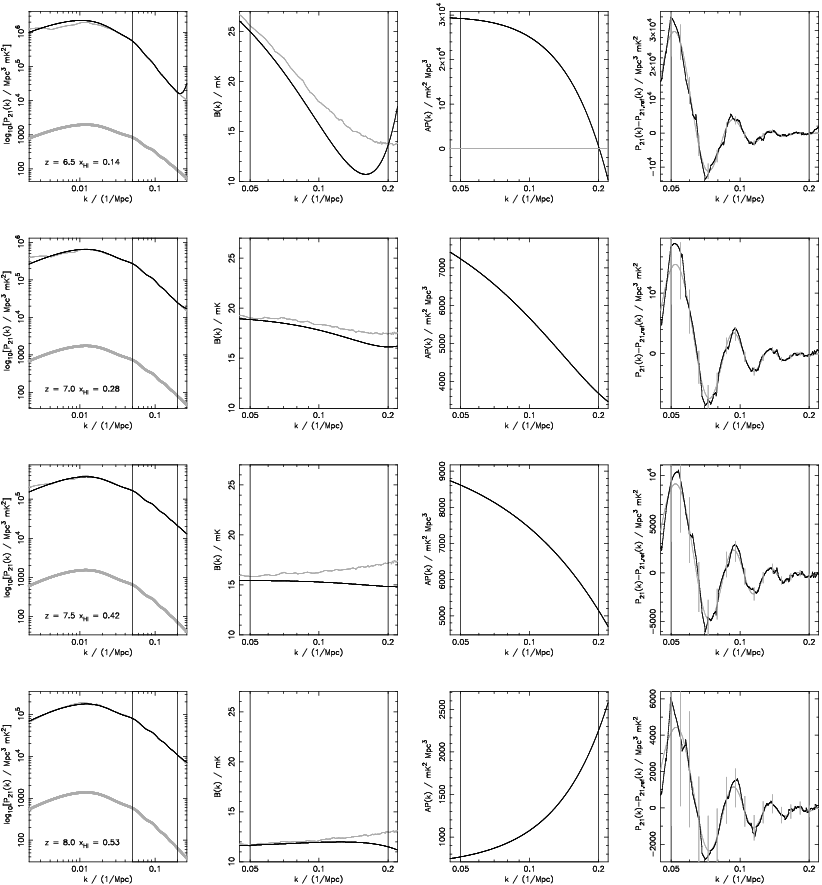
In Figure 1 we show the model 21 cm PS at , 7, 7.5 and 8, corresponding to average volume weighted neutral fractions . The left-hand panels show the ionised gas distribution from the semi-numerical simulations for a box with side length 3 Gpc (co-moving). The panels in the second column show the spherically averaged model 21 cm PS (grey lines). The panels in the third column show the model 21 cm bias (grey lines). The far right-hand panels show the BAO component of the PS, defined as the difference between the 21 cm PS, and a reference 21 cm PS computed from a mass PS without baryons, . The model BAO component, , is shown in grey. The model PS is reproduced in Figure 2.
2.3 Fitting formula for 21 cm power spectra
Following Seo & Eisenstein (2005) we parametrize the fit to the semi-numerical model of the spherically averaged 21 cm PS as
| (5) |
where is a term to describe anomalous power and is the fitted bias in units of mK. The “dilation” or “phase” parameter allows for a dilation/contraction of the matter PS used to fit the 21 cm PS. In our case the input value of is unity since we are assuming we know the cosmological parameters governing . Seo & Eisenstein (2005) note that for the parametrization the PS in equation (5), the errors in the known values of the wave-number dilation parameter directly translate into the errors in the measured BAO scales. In Section 4.2 we calculate the expected redshift dependent errors for an observational campaign which is described in Section 3 below.
The anomalous power term allows for the distortion of the matter power-spectrum due to non-linear mode coupling. Seo & Eisenstein (2005) find that by subtracting a smooth function () from the matter PS derived from their N-body simulations, they are able to recover the shape of the matter PS and thus the BAO signal. Our semi-numerical model is intrinsically linear, and so does not include anomalous power. However we explore the possible effect of anomalous power on the measurement of the BAO scale by including the correction term in the fitted PS. Inclusion of this term approximates the effect of degeneracy between anomalous power and scale dependent bias. In this paper we present results using fits both with and without the term. Note that the degeneracy between the parameters governing the anomalous power and bias terms means that the polynomial fits to these functions cannot be interpreted physically when the term is included (see Section 4). However we find that this degeneracy does not significantly hinder the determination of .
More detailed cosmological constraints may be obtainable if the line-of-sight and transverse BAO scales could be measured independently [see Wyithe et al. (2008) and references therein, and also Okumura et al. (2008), Gaztanaga et al. (2008a) and Gaztanaga et al. (2008b) for recent constraints from galaxy surveys]. Indeed, a low-frequency array is naturally suited to measuring both the line-of-sight and transverse components of the 21 cm PS (see Section 3). Such an analysis would require modelling of the peculiar velocity effects which give rise to the angular dependence of the 21 cm PS in equation (3). As mentioned, the model adopted for the 21 cm PS does not include peculiar velocities. However we note that above fitting formula could be readily generalised to characterise the ionisation and cross density-ionisation power-spectra needed to describe the angular dependence in equation (3). This would allow constraints on the dilation parameter, and therefore the BAO scale, both perpendicular and parallel to the line-of-sight to be extracted from the 21 cm power-spectrum. The signal-to-noise ratio estimates in Wyithe et al. (2008) suggest that the MWA5000 will be similarly sensitive to each of these scales.
3 Measurement of 21 cm power spectra

In this section we discuss the sensitivity of a low-frequency array to the 21 cm PS. The sensitivity to the PS depends on the array design (e.g. total collecting area and antenna distribution) as well as the observation strategy (e.g. total integration time). We consider a low-frequency array which would be a 10-fold extension of the MWA. We refer to this array as the MWA5000 (McQuinn et al., 2006). The MWA5000 would consist of 5000 antennae (with each antenna composed of a tile of cross-dipoles) with effective collecting area m2, where m is the observed wavelength. The dipoles will be sensitive to a wide range of frequencies which translate into redshifts spanning the expected extent of reionisation. However, we assume that the receiver will limit the bandpass to a selected MHz window per observation. We assume that the antennae are distributed with constant density in a core of radius m (within which the - coverage is very high), with the remainder distributed with a radially symmetric density profile out to a radius of km (so that the maximum baseline is km).
We use the prescription from Bowman et al. (2006) for the 3d sensitivity of an array to the 21 cm PS. The array sensitivity is expressed in terms of the wave-vector components which are orthogonal and parallel to the line-of-sight. The modulus of the wave-number is then given by . The sensitivity at large depends crucially on the angular resolution of the array (and therefore the maximum baseline), the bandpass over which the measurement is made , the integration time , and the density of baselines which measure a particular -mode. The noise may be divided into two distinct components. The thermal noise component is proportional to the sky temperature, where K at the frequencies of interest, and may be written
| (6) |
where is the co-moving distance to the centre of the survey volume which has a co-moving depth . Here is the density of baselines which observe a wave-vector with transverse component . In the denominator denotes the number of modes observed in a -space volume . In terms of the -vector components, where is the observed volume. Note that this calculation of incorporates the fact that -modes which do not fit in the bandpass are not observable. The sample variance component of the noise is given by . The sensitivity will improve with the square root of the number of independent fields observed. The total noise may therefore be expressed by
| (7) |
For the purposes of constraining the parameters in equation (5), we average equation (7) over the viewing angle to obtain the spherically averaged noise . Note that this calculation assumes perfect foreground removal over a bandpass with width [see McQuinn et al. (2006) for a discussion of the relationship between foreground removal and bandpass width]. In Section 4 we explore the effect of the choice of on the errors in the measurement of .
We assume that the spherically averaged PS is measured in logarithmically spaced intervals with end points in the range 0.05 Mpc Mpc-1. Wave-numbers below this range would not fit within the nominal bandwidth of MHz at the redshifts of interest. Above Mpc-1 the BAO signal becomes very weak and the matter PS may be non-linear. The binning in -space, which is approximately equivalent to bin widths of , is motivated by the scale of the expected BAO features. For clarity the grey error bars in Figures 1 and 2 represent the uncertainty on the spherically averaged PS for larger spectral bins with width . We assume that three fields are observed () for 1000 hrs each. Given the field of view at these redshifts, this would correspond to surveying a few per cent of the sky.
4 Fits to 21 cm power spectra
In this section we describe the results of fits to the modelled 21 cm PS using the parametrized form in equation (5).
4.1 minimization
We adopt the function as an indicator for the “goodness of fit” of our model,
| (8) |
where and is a vector containing the model parameters. The index refers to the discrete values of corresponding to each data bin (see Section 3). We restrict our fitting to the range MpcMpc-1.
We have adapted the Numerical Recipes routines (Press et al., 1992) which implement the Levenberg-Marquardt technique to iteratively find the parameter set which minimizes the function for a model which is non-linear in its parameters . In Figures 1 and 2 we show the resulting fits for the cases with a third order polynomial bias (black lines), with and without a quadratic anomalous power term respectively. The panels in the second column of Figure 1 (and the first column in Figure 2) show the fitted spherically averaged 21 cm PS as well as the linear matter PS. The panels in the third column of Figure 1 (and second column of Figure 2) show the fitted 21 cm bias. In Figure 2 the panels in the third column show the fitted term (note that the input term is zero since non-linear effects are not incorporated into the semi-numeric code we have used to generate the ionisation maps). The far right-hand panels in each of Figures 1 and 2 show the BAO component of the fitted PS, . The noise in the fitted BAO component is due to the noise in the model calculation of the bias .
 |
 |
The fit to the 21 cm PS is very good in all cases. When the anomalous power term is included there is a trade-off between the power in the 21 cm PS associated with the bias and that due to , indicating some degeneracy. However as we show in the next subsection, this degeneracy does not significantly bias the constraints on the BAO scale. It may of course be possible to alleviate the degeneracies between the bias and the parameters by putting some physically/numerically motivated priors on the values of and .
4.2 Uncertainty in the measured BAO scale
 |
 |
After marginalising over the remaining fit parameters, we may interpret the error in for our fits as the fractional uncertainty in the measurement of the BAO scale (Seo & Eisenstein, 2005). The Fisher matrix is given by (Tegmark et al., 1997)
| (9) |
where is the dimension of and all derivatives are evaluated using the best-fitting . Since we expect the noise in 21 cm PS to be Gaussian, we may invoke the Cramer-Rao theorem to estimate the 1 ( per cent) confidence interval around the best-fitting value of from . Assuming that all other parameters are marginalised over this implies errors around the best-fitting values for of
| (10) |
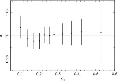
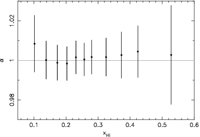
In Figure 3 we plot the the best-fitting values of and the associated 1 error as calculated in equation (10) for several redshifts in the range corresponding to average neutral fractions of for our reionisation model. The left panel of Figure 3 assumes a fitted 21 cm PS with no anomalous power term, whereas the fitted PS used to generate the plot in the right panel includes the term. In each panel the grey horizontal line indicates the input value . Note that the recovered values of deviate from the input values at (). However for the observing strategy and -space binning chosen, this deviation is within the estimated statistical error (although only just at where the neutral fraction is per cent). As reionisation nears completion (), the 21 cm bias becomes most strongly scale dependent in the range 0.05 Mpc Mpc-1. The increasing systematic error toward is therefore a result of the (relatively) low noise level in the 21 cm PS at these redshifts combined with the increasingly strong evolution of the bias function within the fitted range of -values.
We find that the statistical errors are slightly larger when we include the extra parameters required to describe the anomalous power (since the matrix is not diagonal). We note that our estimate of the attainable errors on the phase/dilation parameter are a minimum in the sense that we have assumed perfect foreground removal across each bandpass with width 8 MHz for a total bandwidth of 32 MHz, and we have invoked the Cramer-Rao theorem regarding the minimum 1 error on a parameter from the Fisher matrix of the best-fitting model.
The bandpass over which foreground removal can be performed may affect the errors on the model parameters, even for a fixed total bandpass , because the removal of foreground on larger scales allows for more of the strong large-scale (small ) BAO peaks to be included in the fit. However we find that at the high redshifts that we are considering, increasing above 8 MHz has little affect on the errors in the recovered values of . On the other hand, we find that decreasing increases the systematic uncertainty in the recovered values of toward the end of reionisation. For model fits without the term, the systematic error exceeds the statistical error when (corresponding to redshifts ), indicating that our maximum likelihood indicator is biased. This highlights the potentially significant advantages of including the larger scales accessible with wider bandpasses .
The systematic component of the errors will in general be sensitive to the functional form chosen to describe the 21 cm PS. We find that the effect of increasing the order of the polynomial used to fit the bias is somewhat degenerate with the chosen value of . For example, with coarser k-space binning of the errors in decrease by per cent when the bias is modelled by a fourth order polynomial rather than a third order polynomial. This effect is not observed for (see Figures 3 and 4). This implies that sampling of the BAO features must be sufficiently fine. However, the affect of on the systematic errors in is only significant for when the bias is evolving strongly over the range of fitted k-values.
5 Summary and conclusions
There has been recent interest in the utility of redshifted 21 cm fluctuations from the IGM as a probe of the mass PS at a range of redshifts (McQuinn et al., 2006; Bowman et al., 2006; Mao et al., 2008; Wyithe et al., 2008; Chang et al., 2008; Mao & Wu, 2008, e.g.). During the reionisation era (), the appearance of HII regions generates scale dependence of the bias relating the 21 cm PS to the linear PS. In this paper we have set out to test the extent to which the scale dependence of the 21 cm bias will interfere with the ability to extract the BAO scale from the PS of 21 cm fluctuations.
We have utilised the results of semi-numerical models for the evolution of the ionised hydrogen distribution on large scales in order to construct an estimate for the 21 cm PS at high redshift. For a model in which the IGM is fully reionised by , and assuming the design parameters for a 10-fold expansion the the MWA, we find that the scale dependent 21 cm bias limits the precision, but not the accuracy, of measurements of the BAO scale in the window . We parametrize the bias and anomalous power terms in the 21 cm PS as polynomials, and for the telescope design assumed, find errors on the spherically averaged BAO scale of per cent in the window . At redshifts closer to the end of reionisation, the strong scale dependence of the 21 cm bias introduces systematic error in the BAO scale, which exceeds the level of the statistical uncertainty for narrower bandpasses (). We find that the sensitivity of a low-frequency array to the spherically averaged BAO scale decreases with increasing redshift, becoming per cent by .
The details of the quantitative results presented in this paper are sensitive to the reionisation model assumed. More generally, the constraints available at a particular redshift will be sensitive to the details of the reionisation history. The best constraints are likely to be derived from observations of the Universe when the IGM is per cent ionised - at which time the fluctuations are maximised (Lidz et al., 2008) - but the bias is relatively weakly dependent on scale at the scale of the BAO signal (and hence does not introduce a large systematic error). As a result, if reionisation completes earlier than , the most precise constraints will be obtained at higher redshift than reported here. However, as the foregrounds become brighter when observing at higher redshift, an early reionisation scenario would decrease the maximal precision with which the BAO scale could be measured.
A detailed analysis of the corresponding constraints on the dark energy equation of state is non-trivial and depends on the functional form assumed (Wyithe et al., 2008). We do not explore the translation of BAO scale to cosmological constraints in this paper. Such an analysis should include independent complementary constraints (e.g. from the CMB), and take account of uncertainties in, for example, the horizon scale (McQuinn et al., 2006; Mao et al., 2008, e.g.). Simple estimates of the cosmological constraints from a high redshift BAO measurement were presented in Wyithe et al. (2008).
In a recent paper Mao et al. (2008) propose a parametrization of the 3d 21 cm PS including peculiar velocity effects which is motivated by the generic form expected for the ionisation PS and ionisation-matter PS. Our analysis of the accuracy with which the BAO scale may be recovered in the presence of a scale dependent 21 cm bias is complementary to their detailed discussion of the cosmological constraints available via the redshifted 21 cm PS. Mao et al. (2008) demonstrate that their parametrization can recover the ionisation PS constructed from simulations of reionisation and therefore can be used to constrain cosmological parameters from the 21 cm PS. Whilst they mention that their parametrization struggles to describe the high- ionisation PS by a redshift of when the ionisation PS become significantly scale dependent, this is not found to be a problem up to the Mpc-1 that we consider in this paper. It would be interesting to see how well such a parametrization would perform at the end of reionisation in the wavelength range that we have used for our fits.
Our calculations of the constraints on the BAO scale from 21 cm intensity fluctuations are promising when compared to the expected performance of future galaxy surveys. Glazebrook & Blake (2005) show that a dedicated next-generation spectroscopic galaxy survey could measure the BAO scale to an accuracy of per cent for the transverse component at a redshift , with a slightly reduced sensitivity to the line-of-sight BAO scale. Limitations in the precision achievable arise due to the large number of galaxies needed to reduce the cosmic variance on the scales at which the BAO signal is expected ( Mpc), combined with the decrease in the number of sufficiently luminous galaxies toward higher redshift. The accuracy with which the BAO scale may be measured via the 21 cm intensity PS is immune to both of these constraints because there is no need to resolve individual objects. Redshifted 21cm measurements of the PS will instead be limited by cosmic variance owing to the finite size of the field of view, and sensitivity to individual modes owing to array configuration and finite collecting area. However we find that the PS of redshifted 21 cm fluctuations as measured by the MWA5000 could achieve constraints on the BAO scale at that are comparable to the accuracy which will be available to future galaxy redshift surveys at .
In summary, one potential obstacle to measuring the BAO scale in 21 cm fluctuations during the reionisation era is the strongly scale dependent bias between the 21 cm and mass PS that is produced by the appearance of large ionised regions. In this paper we have shown that the appearance of ionised regions during the reionisation epoch will not inhibit the measurement of the BAO scale during most of the reionisation era.
Acknowledgments
We thank the referee for useful comments. KJR acknowledges the support and hospitality of the Department of Physics, University of Melbourne, and a visiting postgraduate Marie Curie Fellowship hosted by MPA. The research was supported by the Australian Research Council (JSBW). PMG acknowledges the support of an Australian Postgraduate Award.
References
- Angulo et al. (2008) Angulo R. E., Baugh C. M., Frenk C. S., Lacey C. G., 2008, MNRAS, 383, 755
- Barkana & Loeb (2005a) Barkana R., Loeb A., 2005a, ApJ, 624, L65
- Barkana & Loeb (2005b) —, 2005b, ApJ, 626, 1
- Blake & Glazebrook (2003) Blake C., Glazebrook K., 2003, ApJ, 594, 665
- Bowman et al. (2006) Bowman J. D., Morales M. F., Hewitt J. N., 2006, ApJ, 638, 20
- Chang et al. (2008) Chang T.-C., Pen U.-L., Peterson J. B., McDonald P., 2008, Physical Review Letters, 100, 091303
- Cole et al. (2005) Cole S., Percival W. J., Peacock J. A., Norberg P., Baugh C. M., Frenk C. S., Baldry I., Bland-Hawthorn J., Bridges T., Cannon R., Colless M., Collins C., Couch W., Cross N. J. G., Dalton G., Eke V. R., De Propris R., Driver S. P., Efstathiou G., Ellis R. S., Glazebrook K., Jackson C., Jenkins A., Lahav O., Lewis I., Lumsden S., Maddox S., Madgwick D., Peterson B. A., Sutherland W., Taylor K., 2005, MNRAS, 362, 505
- Corasaniti et al. (2007) Corasaniti P.-S., Huterer D., Melchiorri A., 2007, Phys. Rev. D, D75, 062001
- Crocce & Scoccimarro (2008) Crocce M., Scoccimarro R., 2008, Phys. Rev. D, 77, 023533
- Eisenstein (2002) Eisenstein D., 2002, in Astronomical Society of the Pacific Conference Series, Vol. 280, Next Generation Wide-Field Multi-Object Spectroscopy, Brown M. J. I., Dey A., eds., pp. 35–+
- Eisenstein et al. (1998) Eisenstein D. J., Hu W., Tegmark M., 1998, ApJ, 504, L57+
- Eisenstein et al. (2005) Eisenstein D. J., Zehavi I., Hogg D. W., Scoccimarro R., Blanton M. R., Nichol R. C., Scranton R., Seo H.-J., Tegmark M., Zheng Z., Anderson S. F., Annis J., Bahcall N., Brinkmann J., Burles S., Castander F. J., Connolly A., Csabai I., Doi M., Fukugita M., Frieman J. A., Glazebrook K., Gunn J. E., Hendry J. S., Hennessy G., Ivezić Z., Kent S., Knapp G. R., Lin H., Loh Y.-S., Lupton R. H., Margon B., McKay T. A., Meiksin A., Munn J. A., Pope A., Richmond M. W., Schlegel D., Schneider D. P., Shimasaku K., Stoughton C., Strauss M. A., SubbaRao M., Szalay A. S., Szapudi I., Tucker D. L., Yanny B., York D. G., 2005, ApJ, 633, 560
- Furlanetto (2006) Furlanetto S. R., 2006, MNRAS, 371, 867
- Furlanetto et al. (2004) Furlanetto S. R., Zaldarriaga M., Hernquist L., 2004, ApJ, 613, 16
- Gaztanaga et al. (2008a) Gaztanaga E., Cabre A., Hui L., 2008a, ArXiv e-prints, 0807.3551
- Gaztanaga et al. (2008b) Gaztanaga E., Miquel R., Sanchez E., 2008b, ArXiv e-prints, 0808.1921
- Geil & Wyithe (2008) Geil P. M., Wyithe J. S. B., 2008, MNRAS, 386, 1683
- Giannantonio et al. (2008) Giannantonio T., Scranton R., Crittenden R. G., Nichol R. C., Boughn S. P., Myers A. D., Richards G. T., 2008, ArXiv e-prints, 0801.4380
- Glazebrook & Blake (2005) Glazebrook K., Blake C., 2005, ApJ, 631, 1
- Hu & Haiman (2003) Hu W., Haiman Z., 2003, Phys. Rev. D, 68, 063004
- Kaiser (1987) Kaiser N., 1987, MNRAS, 227, 1
- Komatsu et al. (2008) Komatsu E., Dunkley J., Nolta M. R., Bennett C. L., Gold B., Hinshaw G., Jarosik N., Larson D., Limon M., Page L., Spergel D. N., Halpern M., Hill R. S., Kogut A., Meyer S. S., Tucker G. S., Weiland J. L., Wollack E., Wright E. L., 2008, ArXiv e-prints, 0803.0547
- Lidz et al. (2008) Lidz A., Zahn O., McQuinn M., Zaldarriaga M., Hernquist L., 2008, ApJ, 680, 962
- Mao & Wu (2008) Mao X.-C., Wu X.-P., 2008, ApJ, 673, L107
- Mao et al. (2008) Mao Y., Tegmark M., McQuinn M., Zaldarriaga M., Zahn O., 2008, Phys. Rev. D, 78, 023529
- McDonald & Eisenstein (2007) McDonald P., Eisenstein D. J., 2007, Phys. Rev. D, 76, 063009
- McQuinn et al. (2007a) McQuinn M., Lidz A., Zahn O., Dutta S., Hernquist L., Zaldarriaga M., 2007a, MNRAS, 377, 1043
- McQuinn et al. (2007b) —, 2007b, MNRAS, 377, 1043
- McQuinn et al. (2006) McQuinn M., Zahn O., Zaldarriaga M., Hernquist L., Furlanetto S. R., 2006, ApJ, 653, 815
- Mesinger & Furlanetto (2007) Mesinger A., Furlanetto S., 2007, ApJ, 669, 663
- Okumura et al. (2008) Okumura T., Matsubara T., Eisenstein D. J., Kayo I., Hikage C., Szalay A. S., Schneider D. P., 2008, ApJ, 676, 889
- Page et al. (2003) Page L., Nolta M. R., Barnes C., Bennett C. L., Halpern M., Hinshaw G., Jarosik N., Kogut A., Limon M., Meyer S. S., Peiris H. V., Spergel D. N., Tucker G. S., Wollack E., Wright E. L., 2003, ApJS, 148, 233
- Percival et al. (2007) Percival W. J., Cole S., Eisenstein D. J., Nichol R. C., Peacock J. A., Pope A. C., Szalay A. S., 2007, MNRAS, 381, 1053
- Press et al. (1992) Press W. H., Teukolsky S. A., Vetterling W. T., Flannery B. P., 1992, Numerical recipes in C. The art of scientific computing. Cambridge: University Press, —c1992, 2nd ed.
- Seljak & Zaldarriaga (1996) Seljak U., Zaldarriaga M., 1996, ApJ, 469, 437
- Seo & Eisenstein (2003) Seo H.-J., Eisenstein D. J., 2003, ApJ, 598, 720
- Seo & Eisenstein (2005) —, 2005, ApJ, 633, 575
- Seo & Eisenstein (2007) —, 2007, ApJ, 665, 14
- Seo et al. (2008) Seo H.-J., Siegel E. R., Eisenstein D. J., White M., 2008, ArXiv e-prints, 0805.0117
- Shaw & Lewis (2008) Shaw J. R., Lewis A., 2008, ArXiv e-prints, 0808.1724
- Simpson & Bridle (2006) Simpson F., Bridle S., 2006, Phys. Rev. D, 73, 083001
- Spergel et al. (2007) Spergel D. N., Bean R., Doré O., Nolta M. R., Bennett C. L., Dunkley J., Hinshaw G., Jarosik N., Komatsu E., Page L., Peiris H. V., Verde L., Halpern M., Hill R. S., Kogut A., Limon M., Meyer S. S., Odegard N., Tucker G. S., Weiland J. L., Wollack E., Wright E. L., 2007, ApJS, 170, 377
- Tegmark et al. (1997) Tegmark M., Taylor A. N., Heavens A. F., 1997, ApJ, 480, 22
- Trac & Cen (2007) Trac H., Cen R., 2007, ApJ, 671, 1
- Wyithe et al. (2008) Wyithe J. S. B., Loeb A., Geil P. M., 2008, MNRAS, 383, 1195
- Wyithe & Morales (2007) Wyithe J. S. B., Morales M. F., 2007, MNRAS, 379, 1647
- Zahn et al. (2007) Zahn O., Lidz A., McQuinn M., Dutta S., Hernquist L., Zaldarriaga M., Furlanetto S. R., 2007, ApJ, 654, 12