On a worldsheet dual of the Gaussian matrix model
Abstract:
We discuss a modification of Gopakumar’s prescription for constructing string theory duals of free gauge theories. We use this prescription to construct an unconventional worldsheet dual of the Gaussian matrix model.
Keywords:
AdS/CFT, Matrix models1 Introduction.
Since the seminal work of ’t Hooft [1] it has been widely believed that large gauge theories (with adjoint matter fields) should have a dual description in terms of closed strings. Any correlator in a gauge theory has the following expansion
| (1) |
where is the ’t Hooft coupling. This expansion has the same structure as a closed string perturbation theory with . Of course by now we have many examples of this duality, the correspondence [2] and the geometric transition [3, 4] being the most widely studied in recent years. However, an interesting question, still remaining open, is how to build a concrete string theory dual for a given field theory.
In principle, a way to construct a string dual for a given theory is to know the dual of a free field theory and then to turn on non-zero couplings. In case of gauge theories in this program can be pursued in some sense. The free (Gaussian) matrix model is related to a matter coupled to Liouville theory [5, 6], or equivalently to the topological gravity [7, 8, 9, 10]. The other critical matrix models can be obtained by turning on certain perturbations (see [11, 12] for reviews on the subject). However, in dimensions higher than this kind of relation has not been constructed yet.11 1 See for instance [13, 14, 15, 16, 17] for different approaches to the problem.
A very interesting prescription for constructing a stringy dual of a free field theory was proposed by Rajesh Gopakumar [18, 19] (the proposal was further investigated in [20, 21, 22, 23, 24]). The basic ingredient for building the duality in Gopakumar’s proposal is the well known isomorphism [25] between the moduli space of Riemann surfaces and the space of metric graphs. This isomorphism has already appeared in many string theory contexts, like string field theory [26] and different matrix models (the Penner model [27] and the Kontsevich model [28] are the standard examples, see also [29] for a recent review).
The basic idea of Gopakumar’s prescription is to think of every Feynman graph contributing to a given correlator as a metric graph, with the metric given by the Schwinger parameters. Then, the integration over the Schwinger parameters is mapped to an integration over the moduli space of Riemann surfaces and the integrand is interpreted as a worldsheet correlator.
Using Gopakumar’s prescription one can compute several simple correlators [21, 22]. These computations give rise to some interesting questions about the prescription. Namely, there are global symmetries of the gauge theory not realized globally on the worldsheet and some of the correlators localize on sub-manifolds of the moduli space of Riemann surfaces. These issues can be traced to choosing the metric on the Feynman graphs to be defined through the Schwinger parameters. An important question is whether there are different, and yet interesting, choices of the metric.
In this paper we investigate a certain change of the metric assignment to the Feynman graphs, a choice which does not involve the use of Schwinger parameters. We will see in what follows that this choice of the metric ties Gopakumar’s prescription closer to the much studied cases of the matrix models. In particular we will make an attempt to explicitly construct a worldsheet dual of the Gaussian matrix model.
The rest of the paper is organized as follows. In section 2 we discuss the different issues arising from Gopakumar’s prescription. In section 3 we introduce an alternative prescription to define a metric on the Feynman graphs. In section 4 a worldsheet model for the Gaussian matrix model is built based on the alternative prescription. In section 5 we discuss our results.
2 Gopakumar’s prescription with Schwinger parameters.
Let us begin by briefly reviewing the essentials of Gopakumar’s prescription [19] (a detailed review of the prescription can be also found in [21]). For simplicity we discuss a free gauge theory in dimensions containing a single scalar field in the adjoint representation of the gauge group. A generic correlator of gauge invariant operators in this theory has the following form (again for simplicity we discuss only single trace operators)
| (2) |
The above correlator is computed by the different Wick contraction in the free theory. Each Feynman diagram is simply a product of free propagators
| (3) |
Here is the free propagator and is the number of the different Wick contraction of operators and . Note that in the product is also restricted to by normal ordering. However, in matrix models the self contractions are allowed and this restriction is lifted. A particular way to transform each Feynman graph to a metric graph utilized by Gopakumar [19] is to endow each propagator with a length parameter by representing the propagators in the following way
| (4) |
which is simply a variant of the Schwinger parametrization of the propagator.22 2 Of course there are many similar choices of Schwinger parametrization. The original prescription of [19] was written in the momentum space. Then, a contribution from a specific Feynman graph to a correlator is given by
| (5) |
where counts the different propagators connecting given two operators and is the number of these propagators. An important step in the prescription is to transform the above integral over the Schwinger parameters to an integral over a reduced set of parameters . The reduced set of propagators is defined by gluing together homotopically equivalent propagators. After this gluing the expression (5) can be rewritten as
| (6) |
where counts homotopically inequivalent propagators connecting two operators. The parameters are the numbers of homotopically equivalent propagators glued together, and satisfy
After following the above steps we have transformed a Feynman diagram to a metric graph which we will refer to as a skeleton graph. There are two parameters associated with each edge, a Schwinger parameter which defines the metric on the graph, and an additional integer parameter .
The prescription then utilizes Strebel’s theorem [25, 30, 31] (see appendix A for a very brief introduction to Strebel differentials) to rewrite the expression (6) as an integral over the moduli space of punctured Riemann surfaces ,
| (7) |
where are the coordinates on the moduli space. We use this theorem as follows. The dual of the skeleton graph is interpreted as the critical graph of a Strebel differential defined on a Riemann surface of genus (where the genus is specified in the obvious way by the graph) with punctures.33 3 Note that this identification makes it clear why it is needed to go from Feynman graphs to skeleton graphs, as the critical curves of the Strebel differentials contain only vertices of valence three or higher. We will discuss a generalization of this point in what follows. Following the theorem, a specific set of lengths of the edges of the graph, given in Gopakumar’s case by , is translated to a particular point in the space . One then is in position to translate the integration over to integration over . After explicitly performing the integrals over the integrand, , is interpreted as a correlator defining a putative string dual of our free gauge theory. The parameters are quantum numbers of the operators, and the numbers parametrize different Feynman diagrams contributing to a specific correlator.
After defining a prescription to translate field theory correlators to correlators one can try to compute some specific quantities. Although the above prescription is very straightforward, it is quite complicated to use in practice. The main difficulty being computing concrete Strebel differentials to explicitly make the transition between the integration variables. Nevertheless, some simple field theory diagrams can be explicitly translated to the string theory language [21, 22, 23]. In what follows we will be interested in specific issues arising from these simple calculations.
The first issue is the localization of some of the putative correlators obtained via Gopakumar’s prescription on submanifolds of . The reason for this can be understood as follows. The real dimension of is
| (8) |
The number of real parameters coming from a skeleton graph is equal to the number of edges in that graph. A generic dual skeleton graph will have only valent vertices. Obviously if we have vertices of a larger valence the number of edges will be reduced (we do not have vertices of valence as the skeleton does not have homotopically equivalent edges). In such a graph the number of vertices, , is related to the number of edges, , by . The number of faces of the dual graph is the number of operators . Then using the relation we get the number of real parameters in a generic skeleton graph to be , in agreement with (8).
However, any correlator might get contribution not just from generic graphs but also (or only) from non-generic ones, having valent vertices in the dual graph. These diagrams will have less parameters and thus after the change of variables via the Strebel theorem we will get integrals over submanifolds of . For particular diagrams the integration will be even restricted to submanifolds of [21, 22, 23].

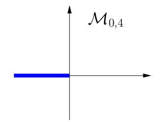

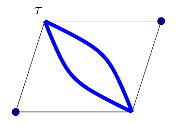
Although we are not used to deal with correlators which localize on sub-manifolds of the moduli space, one can think of mechanisms responsible for this fact in an otherwise well behaved s. One such mechanism was described in [23].
It is amusing that in some cases (in the cases depicted in figure 1, the sphere case but not the torus one) having the localizations might be a signal that some OPE limits are not allowed as some of the vertices do not have Wick contraction between them on the field theory side [23] (for more details on the relation between space-time and worldsheet OPE consult [32]).
The second issue arising from Gopakumar’s prescription is the realization of the special conformal symmetry of the gauge theory on the worldsheet. If we take the free theory under discussion to be scale invariant (i.e. no mass terms), the theory might also be conformal, as it happens for gauge theories in four dimensions. The theory will then posses a larger symmetry which will include the dilatation transformations and special conformal transformations. The worldsheet operators built via Gopakumar’s prescription will have well defined dilatation properties and this symmetry will not act on the worldsheet coordinates. This is easily seen from (6) for instance. The dilatation amounts to the simultaneous rescaling of all the Schwinger parameters by a common factor. This rescaling means that the corresponding Strebel differential is rescaled. The point on defined by a Strebel differential is not affected by this rescaling and thus the only effect of it is the overall rescaling of the correlator as expected. On the other hand, the action of the special conformal transformations is non trivial on the worldsheet. As this action involves the space time coordinates , it will act differently on the different Schwinger parameters and will change the Strebel differential corresponding to each graph, thus taking us to different points on . This property does not invalidate Gopakumar’s prescription, but makes any comparison of the obtained results to other approaches to gauge/string duality, like the standard approach [2], more difficult.
In the following section we will discuss how a change in the metric associated to the Feynman graphs can affect the above listed properties.
3 Mapping graphs to Moduli space without Schwingers.
To use Strebel theorem to map gauge theory correlators to worldsheet expressions we had to treat Feynman diagrams as metric graphs. As we described above R. Gopakumar has suggested to take Schwinger parameters as the metric. Obviously, one has a considerable amount of freedom in rewriting propagators in terms of Schwinger-like parameters.
As an example consider the following. We could define the Schwinger parameters directly on the skeleton graph and not on the original Feynman diagrams,
| (9) |
and treat the parameters appearing here as the metric. The putative string theory expressions would be altered. The above prescription gives us also a natural way to avoid localizations. We can define a parameter for all possible contractions in the skeleton graph. If some contraction does not appear in a specific Feynman graph then the corresponding vanishes and the Schwinger integral integrates to . In this way we can associate a maximal number of Schwinger parameters for each Feynman graph and thus completely avoid the issue of localizations.44 4 Of course the above prescription has to be defined more carefully. For instance, a given skeleton can be a subdiagram of different “maximal” graphs. However, there are at least two problems even with this prescription. First, as we associate metric parameters coupled to the space-time coordinates the space-time special conformal symmetry still remains a problem. Second, any relation between space-time and worldhseet OPE naively is lost.
The above example teaches us quite a generic lesson. Avoiding localizations means having enough parameters on the metric graph to correspond to the real dimension of and this will make the relation between the space-time OPE and worldsheet OPE problematic. We do expect such a relation to exist from the standard examples [32]. Moreover, for the space-time special conformal transformations not to act on the worldsheet coordinates the metric parameters on the skeleton graphs should be decoupled from the space-time coordinates.
In what follows we will describe a prescription which will cure the issue of conformal invariance but it will come at the price that now all correlators in a putative string dual to a free gauge theory will localize on a discrete set of points in .
The way to restore the space time symmetries is to avoid direct coupling between the space time variables and the length parameters of the metric graphs as discussed above. Essentially, there is a natural way to associate a length parameter to an edge of a skeleton of a Feynman graph without Schwinger parameters. As we saw in the previous section, any such edge has an integer parameter, its multiplicity . We can define a metric on each skeleton graph using these integer parameters. Let us consider a correlator
| (10) |
For each Feynman diagram contributing to it we build a skeleton graph as before. For each edge of the skeleton we specify a length given by its multiplicity, . The parameters obviously satisfy
| (11) |
Thus, we identify the parameters with the circumferences of the Strebel differential poles. In this way we will map each diagram to a discrete set of points in . Thus, any correlator (restricted to a given Riemann surface) in a putative string dual of the above prescription will get contributions from a set of points in the moduli space.55 5 Note that this prescription retains a very weak relation between the space-time and worldsheet OPEs. Namely, as in Gopakumar’s original prescription, an absense of some OPE limit in space-time will imply some restrictions on the possible contributions from different regions of the moduli space.
To conclude this section we comment on the important issue of turning on the interactions. First, as we will consider correlators of operators with higher dimensions we will get contributions from more Feynman diagrams and thus more points of the moduli space will be covered. Essentially, any Strebel differential (up to an unimportant over-all scaling) can be approximated by a differential with integer edge lengths (see [33] for thorough discussion of Strebel differentials with integer lengths). Thus as we increase the dimensions of the operators one should get contributions from a dense set of points on .
After turning on interactions, infinite number of points of the moduli space will contribute. However, here it is not a-priori clear whether the covering will be dense. If the covering is dense, then the string theory expressions will be discontinuous on the moduli space (at least for arbitrary small couplings in the gauge theory). At each order of the perturbative expansion we will have a finite number of points and a value of the integrand will be proportional to some power of the coupling constants. If the covering is dense then in any vicinity of a given point infinite number of orders of the perturbative expansion will contribute. If the couplings are not arbitrarily small then problems might not arise. However, we will have to understand this issue better if we are to describe weakly coupled theories, like the limit of small coupling of the SYM.
4 Toward a worldsheet theory for the Gaussian matrix model.
In this section we will try to gain some understanding of the prescription presented above in the relatively well understood case of the matrix models. In particular we will consider the free, Gaussian, model. Much is known about the relation of this model to string theories. In particular, it is related to the topological gravity [7] and its formulation through Liouville theory with matter [6, 34] (see [35] for reviews). Moreover, there is another matrix model, the Kontsevich model, which is also related to the topological gravity [28]. In a modern perspective the Gaussian model is seen to be related to the theory living on the branes [36] in the above mentioned Liouville theory and the Kontsevich model describes the string field theory on the branes [37]. The Kontsevich model can be obtained through a specific double scaling limit of the loop operator expectation values in the Gaussian matrix theory [38, 39].66 6 See also [40] for yet another connection between the Kontsevich model and the Gaussian theory. In what follows we will not explicitly use (or try to derive) the above connections of the free matrix model to string theory. We will rather just follow the prescription presented in the previous section to explicitly construct a worldsheet dual of a free matrix model.
Let us first briefly outline the main steps of the construction appearing in this section. First (section 4.1), we will use the prescription of the previous section to construct a toy -model which will imitate a string theory structure. The sum over complex structures will be implemented by a sum over a specific set of Strebel differentials dictated by the prescription. We will define an action and a set of operators for this toy model. The action and the operators will be defined in terms of a discrete set of fields associated to the double poles of the Strebel differentials. This model will be explicitly designed to reproduce the Gaussian model correlators. In the following sections we will recast this toy model as a worldsheet theory with an unconventional measure on the moduli space.
4.1 A toy -model.
We consider a gauge invariant correlator of the following form
| (12) |
computed in the Gaussian matrix model with an action given by
| (13) |
where is a hermitian matrix.
This correlator is computed as a sum of the different Wick contractions. It can be naturally expanded in powers of . Every loop gives a factor of , and a propagator gives . All the vertices are external and do not give any factors of . Thus the power of accompanying each diagram contributing to an point correltor (12) is ( is the number of loops and is the number of edges in a given diagram). Thus, a correlator (12) in the free theory can be written as
| (14) |
where summation is over different Feynman graphs and is the number of Wick contractions giving each graph (for instance see [27]). is the number of vertices of power . is th genus and the factor is the symmetry factor of the th Feynman graph (we identify the graphs by mapping the set of vertices and the set of edges onto themselves keeping the orientation of the vertices fixed).
In order to construct a two dimensional model reproducing the field theory result we have to do essentially two things. We have to construct an action and map the field theory operators to vertex operators in the toy -model. We will have a considerable amount of freedom by trading between quantities which will go to the definition of the vertex operators and to the action. We first construct a model with the simplest action and then use the above mentioned freedom to rewrite the expressions in a more familiar way.
Let us first remind ourselves the logic of our prescription. We take a correlator of the form (12) and construct all the possible Feynman diagrams. For each diagram we consider a dual of its skeleton. This skeleton graph has the multiplicities of its edges as the metric of those edges. Finally, due to Strebel theorem there is a unique quadratic differential with this metric graph being its critical graph. Thus, in order to reproduce an point correlator restricted to genus Riemann surface we will have to consider all the possible Strebel differentials with integer edges on the genus surface with marked points, and the residues of the poles being the parameters . We will write an expression doing the job for us and then comment on the nature of different terms. A correlator on surface of genus in a free matrix model is reproduced by the following toy -model
| (15) |
The set is the set of Strebel differentials on a genus Riemann surface with all the edges integer valued and double poles. is the set of the double poles of differential . We identify the operators as
With these identifications we will reproduce exactly the free field theory result (only the connected diagrams counted)
| (22) |
Let us explain different quantities appearing above
- •
The integration over is introduced to equate between the insertion parameter and the circumference of the differential at puncture , .
- •
is a symmetry factor and is computed as follows. Note that each Feynman diagram defines several inequivalent metric graphs and thus is described by a number of points on the moduli space.77 7 However, each metric graph corresponds to a unique Feynman diagram. The inequivalent metric graphs are obtained by assigning labels to the vertices and identifying graphs by mapping the set of vertices and the set of edges onto themselves keeping the orientation of the vertices fixed. We denote by the number of inequivalent metric graphs corresponding to a given Feynman diagram. Thus, to reproduce the combinatorics of (14) we have to define .


Figure 2: Depicted here are two examples of different metric graphs corresponding to the same Feynman diagram. All the edges of the graphs are of length one. On the left we have two metric graphs corresponding to the unique Feynman diagram contributing to ( and ). On the right we have three metric graphs corresponding to the unique diagram of ( and ). - •
The sum over Strebel differentials has to be further constrained in order to not over-count contributions due to the CKVs. For instance, we have to take the sphere Strebel differentials with three of the pole positions fixed to prescribed values.
- •
The binomial coefficients appearing in the operator mapping count homotopycally trivial self contractions of the operators.
- •
The sum over Strebel differentials can be decomposed as follows. Any two differentials having same critical graphs but edges of which differ by a common multiplicative factor correspond to the same location on the moduli space. Thus, the sum over the set of Strebel differentials with integer lengths decomposes into a dense sum over the moduli space times a sum over which encodes the over all integer scale of the differential. Roughly speaking
(23) Here the prime over the integral denotes that the integration is really a dense summation.
In the following sections we will rewrite the above model in a language a bit more familiar from the usual formulations of string theories.
4.2 Enlarging the set of differentials.
In this section we will discuss a useful extension of the set of Strebel differentials defined in the previous section. As we will see in the following section this extension will allow us to rewrite our toy -model in an (almost) conventional string theory language.
The extension we will introduce is basically to add to the set differentials with some of the circumferences exactly zero. There are no Strebel differentials with zero circumferences and thus we should extend the notion of these differentials to include such objects. Essentially, the extension is straightforward. Note that we can add to the set of Strebel differentials limits of differentials with one of the edges going to zero length. Usually this procedure brings two zeros together and produces a zero (with a valence being a sum of the valences of the two original zeros). However, if the edge encircles a double pole (and has both ends ending on the same vertex) then a more interesting scenario can happen. If the edge ends on a zero of valence greater than two the result of taking the limit is a zero of smaller valence. If the zero is of valence two then the result of the limit is a regular point. Thus, the above two limits produce well behaved Strebel differentials. Finally, if the edge ends on a simple zero the result of the limit will be a simple pole and the critical graph will have a single edge emanating from this point. A Strebel differential can not have simple poles and thus we will have to add the above configuration to the differentials we consider.88 8 A discussion of quadratic differentials with simple poles appears also when considering compactifications of moduli spaces. See for instance [31].
Consider the following two simple examples of the differentials that the above procedure produces. Consider the differential
| (24) |
For the critical curve of this differential looks as the left curve on figure 3. By taking we obtain the following differential
| (25) |
and the critical curve is depicted on the right side of figure 3. A second simple example is the case obtained by a different limit of the diagram depicted in 3. One can take one of the circle edges to zero as well as the central edge. This is given by and the differential is simply
| (26) |
Note that introducing simple poles enables us to discuss homotopically trivial self contractions on the same footing as all the other contractions. Thus we will make the following definition of a set of differentials which will be of interest to us. We will denote the set of the Strebel differentials with integer lengths on genus surface with exactly double poles with non-vanishing circumferences and any number of double poles with vanishing circumferences (in the sense discussed above) by . This set extends by allowing differentials with simple poles.
Let us discuss two possible metrics one can put on the worldsheet using a Strebel differential . One natural choice to define a metric is
| (27) |
The curvature tensor of this metric is proportional to and we can write
| (28) |
where ’s are the positions of the poles and the zeros of the differential. The numbers are the multiplicities of these points. That is for a double pole , for a simple pole , for a regular point and for a zero of valence we have . One can check the combinatorics to obtain
| (29) |
Another choice of metric follows directly from the extension of the set of differentials discussed above. Recall how the Strebel differentials entered into the prescription of section 3. These differentials had critical graphs equivalent to the dual graphs of the skeleton of a given Feynman diagram. However, after extending the set of differentials above, it is sensible now to associate for each Feynman diagram itself a differential, which we will denote by . This differential will have the Feynman diagram itself (note, not the skeleton but the diagram itself) as its critical graph. The existence and the uniqueness of such differential is guaranteed by the Strebel theorem and the construction above. In appendix B we explicitly construct the dual for a given differential . The vertices of the critical graph of will become the faces of the critical graph of and vice versa. In the following table the map between the special points of the two differentials is summarized,
Note that the double poles with circumference of are mapped to regular points of and some regular points of can be mapped to double poles of (for details consult appendix B). In what follows when we will refer to a set of special points of a differential (zeros and poles) we will always consider them as defined by the differential.
We can use the differential to define a metric
| (34) |
The curvature computed in this metric has the following form
| (35) |
where are the zeros, simple and double poles of . In the above equation the parameters are defined by the differential and in particular the circumference of a zero (or a simple pole) of is defined to vanish.
4.3 Constructing a worldsheet model.
We are now in position to rewrite our toy -model in a more familiar way. Our action (15) and the definition of operators (4.1) appear as discrete sums over special points on the worldsheet. However, using Strebel differentials we can write these as integrals over the worldsheet.
First we claim that the following model is equivalent to the one defined in section 4.1. The correlators in the model are computed using the following expression
| (36) |
The action is given by
| (37) |
and we identify the operators as
| (38) |
The set is the set of the double poles, and is the set of simple poles and zeros of the differential. The parameter will be shortly identified. We see that with the above identification of the operators is problematic. Thus, we will remove this operator from the theory and restrict the set to differentials with no double poles of circumference two. This set is denoted by in equation (36). We will comment on the interpretation of the operator at the end of this section.
The equivalence of (36) and (15) can be easily established. Note that the integration over for sets exactly as one obtains in the model of section 4.1. Further, the existence of homotopically trivial self-contractions is dealt with by allowing simple poles. Note that a simple pole of the differential implies that the corresponding Feynman diagram has a homotopically trivial self-contraction, and thus summing over all possibilities to have simple poles counts all the different ways to introduce this class of self contractions. The integration over for gives simply an overall factor of , where is the number of faces of the Feynman diagram (which is equal to the number of the double poles of ). The overall and dependence of the correlator is
| (39) |
Thus, by setting the model (36) is equivalent to the model (15) and thus to the Gaussian matrix model.
The reason why we introduce a slightly modified version of our original simple model is that now we can naturally rewrite it in terms of real worldsheet fields. Using the results of the previous subsection we can write the dependent part of the action as ( denote )
| (40) | |||||
Here is a function on the Riemann surface satisfying
| (41) |
In order to define more concretely how to lift the set of s to a field on the worldsheet we will have to define the functional integration measure of this field. To do so we first write the vertex operators as functions of this field
Here is a yet undetermined function of the metrics. Next we denote the appropriate measure for the field by . The functions and the definition of the measure should conspire so that the functional integration will reproduce the discrete integrations of (36). There is a considerable amount of freedom of how to define these quantities. However, one can show (the technical details can be found in appendix C) that the following choice can be made. One can define
| (42) |
where ’s are normalization factors (see appendix C). With this choice the discrete theory is reproduced by the following functional integration
| (43) |
where and is the standard measure for a periodic scalar.
Further, the dependent part of the action can be written as where
| (44) |
and we will refer to this operator as the “puncture” operator. The parameter is defined as
| (45) |
Here is a normalization constant (see appendix C). Note that the definition of the functions for the puncture operator and for the other operators is different. The technical reason for this, as explained in appendix C, is the fact that the puncture operator has to be inserted on the faces of the Feynman diagram and the other operators are inserted at the vertices of the diagram.
Let us summarize our results. The correlators (only connected diagrams counted) of the Gaussian matrix theory are reproduced by the following model. The correlators are given by
| (46) |
The action is
| (47) |
and the operators are
Note that the above theory bares some resemblance to the Itzhaki-McGreevy string theory [41]. In particular it is tempting to identify with the time-like Liouville field of that model (which has ).
To actually prove that the model (46) is equivalent to some kind of string theory we have to understand better the measure on the moduli space. The measure on the moduli space is unconventional and is given by
| (50) |
We did not start by defining our model as an integral over metrics, but it is plausible to guess that the above measure should consist of the integration over the usual moduli space of Riemann surfaces together with some ghost system and an additional matter field(s). It is very interesting to establish whether these can be formulated in terms of a conventional ghost system and a matter field, which should be the real Liouville mode in this model, the one coming from the broken Weyl invariance. A remnant of this Liouville field can be seen in (23) in terms of a discrete rescaling of the Strebel differentials and thus also a rescaling of the metric. In this context, let us comment on the nature of the operator. The fact that we fail to describe this operator on the worldsheet is yet another sign for the need to introduce additional structure to the model. It might be the case that the operator should be defined in terms of the additional worldsheet fields and be independent of the field . We leave the investigation of these issues to future research.
5 Discussion.
In this paper we have introduced a prescription for constructing worldsheet duals of free field theories. This prescription is a variant of the prescription suggested by R. Gopakumar [19]. Using this prescription we have constructed an unconventional worldsheet dual of the free matrix model.
There are many questions which deserve further investigation. First of all, the main issue left open is a better understanding of the moduli space measure. In particular one can wonder whether a string theory in an unconventional gauge might give the measure (50). Making sense of the measure on the moduli space is crucial for making any connection with the familiar formulations of string theories.
Another important direction for further research is to generalize the discussion in section 4 to higher dimensions and to theories with multiple fields. The similarity of our model to the Itzhaki-McGreevy string, which was proposed in [41] as a worldsheet dual of the quantum mechanics of a gauged matrix harmonic oscillator,99 9 See also [42] for a discussion of harmonic oscillator quantum mechanics in the context of gauge/gravity duality. suggests that a better understanding of the moduli space measure might shed some light on the case. Essentially, it is tempting to conjecture that the unconventional worldsheet dual of the Gaussian matrix model obtained in section 4 is really computing a certain class of harmonic oscillator expectation values, and the full string theory extension of this model is the dual string theory of the harmonic oscillator quantum mechanics.
There are at least two new issues with going to . First, the propagators are not trivial any more, i.e. they depend on the space-time coordinates . One can try and use the Fourier tricks of section 4 to deal with this complication. That is, we can introduce additional fields on the worldsheet. For each point of the action for these fields can be defined as a Fourier transform of the corresponding Feynman diagram. The vertex operators thus will include an additional exponential . The challenge then is to write a continuous (and local) action on the worldsheet for the fields .
Another important new issue with going to is the absence of self-contractions in these theories. As the position space propagators diverge when the separation is taken to zero, we have to remove all the self contractions with some kind of normal ordering procedure. Removing self contractions implies that we will have less Feynman diagrams and cover less points on the moduli space. Essentially, the self contractions can be divided into two classes, homotopically trivial and non trivial ones. We saw in section 4.3 that the homotopically trivial self contractions can be naturally taken into account by the puncture operator. Thus, taking away this class of self contractions will probably amount to reconsidering the puncture operator. Taking away the homotopically non trivial self contractions has a more geometric meaning. For instance, the points contributing to any two point correlator on the torus will localize on a submanifold of exactly as it happens in Gopakumar’s prescription [21]. It will be very interesting to understand better the role played by self contractions in this type of constructions.
Acknowledgments.
I am grateful to O. Bergman, R. Gopakumar, A. Pakman, and L. Rastelli for useful discussions and comments on the manuscript. I would especially like to thank O. Aharony and Z. Komargodski for numerous discussions and comments during different stages of this project. This work was supported in part by the National Science Foundation, grant 0653342.Appendix A A short primer on Strebel differentials.
A quadratic differential is the following object,
| (51) |
where is a meromorphic function on a given Riemann surface. This differential is defined to have the following property under a holomorphic reparametrization of the worldsheet ,
| (52) |
Using quadratic differentials one can define a length for a line element through
| (53) |
Note that this length is in general a complex number. It is useful to define the notions of horizontal and vertical curves of the differential. Given a curve on the Riemann surface we say that it is horizontal if
| (54) |
and vertical if the opposite inequality holds. Note that the length of the horizontal curves computed using (53) is real. By convention we will discuss the horizontal curves in what follows. A horizontal curve can either be closed or end on a zero or a pole. The set of all non-closed horizontal curves of a quadratic differential is called the critical curve of the differential. We restrict to quadratic differentials critical curve of which is compact.
If a quadratic differential has at most double poles (with negative coefficients) then the critical curve divides the Riemann surface into ring domains. The vertices of the critical curve of such a differential are the zeros and the simple poles of the differential. The following theorem due to K. Strebel holds,
Given a Riemann surface with marked points and positive numbers associated to those points, there is a unique quadratic differential with double poles as its only singularities such that:
- •
It has exactly double poles located at the marked points
- •
The residues of the double poles are the numbers
- •
The Riemann surface is a union of disc domains defined by the marked points.
We refer to a differential which satisfies the properties above as a Strebel differential. Note that from this theorem follows that there is a unique Strebel differential for each point of . Further, this also gives us a natural isomorphism between the space and the space of metric graphs with faces on genus surface.1010 10 In this context we define a metric graph as a connected graph with a positive real number associated to every edge and all the vertices at least trivalent. For each point of we associate the critical curve of the corresponding Strebel differential as the metric graph (metric on the graph defined through (53)), and the other direction of the isomorphism can be also (less trivially) established.
When explicitly trying to find a Strebel differential for a given Riemann surface and a given set of residues the first two conditions above can be easily satisfied. The third condition is however a very non-trivial one. Essentially, it can be rephrased as the demand that all the distances between the zeros of the differential computed in Strebel metric (53) should be real. Computing these distances will give constraints on the parameters of the differential. Usually these constraints will be expressed through elliptic integrals, which are difficult to solve. In figure 5 an example of a Strebel differential is depicted.
Appendix B The dual Strebel differential .
Given a Strebel differential consider the following quadratic differential
| (55) |
where we have defined
| (56) |
and is one of the zeros of the differential . Note that has correct properties under coordinate transformations. The differential is well defined because all the edges of are integer (and this also implies that has the same periodicity properties as ). Let us consider the behavior of near special points of . First, near a double pole of we have
| (57) |
Using this we obtain
| (58) |
The above implies for that
| (59) |
Thus the differential has a zero of valence where the differential has a double pole with circumference . Consider now a zero of valence of the differential . Near the zero we have
| (60) |
where is some constant. Remember that all the edges of differential have integer lengths by assumption and thus
| (61) |
Thus we obtain for the differential
| (62) |
Thus we conclude that at the positions of the zeros of with valence the differential has double poles of circumference . Moreover, at the regular points on the critical curve of having integer distance from the same argument as above implies that the differential has a double pole with circumference . The differential has no other poles or zeros. We have shown that the differential satisfies all the properties of the dual quadratic differential from section 4.2, and we just have to prove that it also is a Strebel differential.
In order to prove that the differential is Strebel we have to show that all the distances between the zeros of are real. Essentially, we have to prove that the following integrals are real
| (63) |
where and are zeros (or simple poles) of and thus double poles of by construction. Using the fact that , and (55) we obtain
| (64) |
Thus we have shown that is a valid Strebel differential with integer edge lengths. The critical curve of is the Feynman diagram, the skeleton graph of which is dual to the critical curve of . Finally, using (64) one can show that the dual differential of () is ,
| (65) |
As a simple example of the above we consider the following differential ( is the Weierstrass elliptic function1111 11 See for instance [21] for examples of Strebel differentials on a torus.)
| (66) |
We regard this differential as a Strebel differential on a torus with . This differential has two double poles of circumference four and two double zeros in the fundamental domain. We use (55) to find the dual differential
Several additional examples of differentials along with their duals are depicted in figures 6 and 7.
Appendix C Measure details.
On a given Riemann surface with a (dual Strebel) metric we define a complete set of functions
| (68) | |||||
Given a function on a Riemann surface we make the following expansion
| (69) |
The zero mode encodes the fact that the scalar is periodic and takes values in the interval . The standard path integral measure for a scalar field is given by
| (70) |
We want to show that the following path integral measure for the field can be chosen ()
| (71) |
We have to check that with this definition of the measure the results of (36) are reproduced. Let us compute the following quantity (denote ),
| (72) | |||||
Here is the number of puncture operators and is the number of all the other operators. In order for the continuous and the discrete definitions of the model to agree the above has to be a sum of products of Kronecker -functions equating the elements of the set of to the elements of the set . Note also that the path integral above looks very similar to a standard correlator of tachyons in bosonic string theory. The difference is that here the metric (the Strebel metric ) is singular with some of the insertions sitting at the singularities (s). In the standard string theory the above path integral is regularized by normal ordering the operators. However, because some of the operators are inserted at the singularities of the metric this regularization is not effective in our case and we will employ a slightly different one. Thus, let us evaluate (72) directly using (68) and (70)
| (73) |
Note that the exponential appearing in the integrand is almost always zero. This follows from the fact that is the Green’s function on the Riemann surface and it logarithmically diverges when . The only way for the integrand not to vanish is if
| (74) |
Further we will assume that diverges at the positions of the poles of for corresponding to the puncture operator (). A natural (and diff invariant) way to satisfy this assumption is to take . We also assume that diverges at the positions of the zeros of . The natural choice satisfying this is to take . Note (see appendix B) that the poles of the metric and the zeros of are located at the same positions on the worldsheet. Assuming the above (and remembering that the number of zeros and simple poles of is equal to ) the integrand will not vanish only if the set can be element by element equated to the set and the set to be accordingly equated to the set . Thus, we conclude that the integrand of will be proportional to a sum of products of Kronecker -functions.
In order to obtain a finite result for we have to regularize the integrals in (73). For instance, we can restrict to a finite number of and then the exponential in the integrand will be smeared. We can regulate the metrics by cutting small holes around the poles. The exact prescription for the regularization will be encoded in the over-all normalization of the vertex operators. Thus finally, we will define the operators as
| (75) | |||||
The constants and are the normalization constants and their value depends on the explicit regularization procedure used.
References
- [1] G. ’t Hooft, “A planar diagram theory for strong interactions,” Nucl. Phys. B 72, 461 (1974).
- [2] J. M. Maldacena, “The large N limit of superconformal field theories and supergravity,” Adv. Theor. Math. Phys. 2, 231 (1998) [Int. J. Theor. Phys. 38, 1113 (1999)] [arXiv:hep-th/9711200]; S. S. Gubser, I. R. Klebanov and A. M. Polyakov, “Gauge theory correlators from non-critical string theory,” Phys. Lett. B 428 (1998) 105 [arXiv:hep-th/9802109]; E. Witten, “Anti-de Sitter space and holography,” Adv. Theor. Math. Phys. 2, 253 (1998) [arXiv:hep-th/9802150].
- [3] R. Gopakumar and C. Vafa, “On the gauge theory/geometry correspondence,” Adv. Theor. Math. Phys. 3, 1415 (1999) [arXiv:hep-th/9811131].
- [4] H. Ooguri and C. Vafa, “Worldsheet derivation of a large N duality,” Nucl. Phys. B 641, 3 (2002) [arXiv:hep-th/0205297].
- [5] D. J. Gross and A. A. Migdal, “Nonperturbative Two-Dimensional Quantum Gravity,” Phys. Rev. Lett. 64, 127 (1990); D. J. Gross and A. A. Migdal, “A non-perturbative treatment of two-dimensional quantum gravity,” Nucl. Phys. B 340, 333 (1990).
- [6] J. Distler, “2-d quantum gravity, topological field theory and the multicritical matrix models,” Nucl. Phys. B 342, 523 (1990).
- [7] E. Witten, “On the structure of the topological phase of two-dimensional gravity,” Nucl. Phys. B 340, 281 (1990).
- [8] E. Witten, “Two-dimensional gravity and intersection theory on moduli space,” Surveys Diff. Geom. 1, 243 (1991).
- [9] R. Dijkgraaf and E. Witten, “Mean field theory, topological field theory, and multimatrix models,” Nucl. Phys. B 342, 486 (1990).
- [10] E. P. Verlinde and H. L. Verlinde, “A solution of two-dimensional topological quantum gravty,” Nucl. Phys. B 348, 457 (1991).
- [11] P. Di Francesco, P. H. Ginsparg and J. Zinn-Justin, “2-D Gravity and random matrices,” Phys. Rept. 254, 1 (1995) [arXiv:hep-th/9306153]; P. H. Ginsparg and G. W. Moore, “Lectures on 2-D gravity and 2-D string theory,” arXiv:hep-th/9304011.
- [12] I. R. Klebanov, “String Theory In Two-Dimensions,” arXiv:hep-th/9108019.
- [13] K. Bardakci and C. B. Thorn, “A worldsheet description of large quantum field theory,” Nucl. Phys. B 626, 287 (2002) [arXiv:hep-th/0110301]; C. B. Thorn, “A worldsheet description of planar Yang-Mills theory,” Nucl. Phys. B 637, 272 (2002) [Erratum-ibid. B 648, 457 (2003)] [arXiv:hep-th/0203167]; K. Bardakci and C. B. Thorn, “A mean field approximation to the world sheet model of planar field theory,” Nucl. Phys. B 652, 196 (2003) [arXiv:hep-th/0206205]; S. Gudmundsson, C. B. Thorn and T. A. Tran, “BT worldsheet for supersymmetric gauge theories,” Nucl. Phys. B 649, 3 (2003) [arXiv:hep-th/0209102]; K. Bardakci and C. B. Thorn, “An improved mean field approximation on the worldsheet for planar theory,” Nucl. Phys. B 661, 235 (2003) [arXiv:hep-th/0212254]; C. B. Thorn and T. A. Tran, “The fishnet as anti-ferromagnetic phase of worldsheet Ising spins,” Nucl. Phys. B 677, 289 (2004) [arXiv:hep-th/0307203]; K. Bardakci, “Further results about field theory on the world sheet and string formation,” Nucl. Phys. B 715 (2005) 141 [arXiv:hep-th/0501107]; M. Kruczenski, “Planar diagrams in light-cone gauge,” JHEP 0610, 085 (2006) [arXiv:hep-th/0603202]; K. Bardakci, “Field theory on the world sheet: Mean field expansion and cutoff dependence,” [arXiv:hep-th/0701098].
- [14] P. Haggi-Mani and B. Sundborg, “Free large N supersymmetric Yang-Mills theory as a string theory,” JHEP 0004, 031 (2000) [arXiv:hep-th/0002189]; B. Sundborg, “Stringy gravity, interacting tensionless strings and massless higher spins,” Nucl. Phys. Proc. Suppl. 102, 113 (2001) [arXiv:hep-th/0103247]; H. L. Verlinde, “Bits, matrices and ,” JHEP 0312 (2003) 052 [arXiv:hep-th/0206059]; J. G. Zhou, “pp-wave string interactions from string bit model,” Phys. Rev. D 67 (2003) 026010 [arXiv:hep-th/0208232]; D. Vaman and H. L. Verlinde, “Bit strings from N = 4 gauge theory,” JHEP 0311 (2003) 041 [arXiv:hep-th/0209215]; A. Dhar, G. Mandal and S. R. Wadia, “String bits in small radius AdS and weakly coupled N = 4 super Yang-Mills theory. I,” arXiv:hep-th/0304062; K. Okuyama and L. S. Tseng, “Three-point functions in N = 4 SYM theory at one-loop,” JHEP 0408 (2004) 055 [arXiv:hep-th/0404190]; L. F. Alday, J. R. David, E. Gava and K. S. Narain, “Structure constants of planar N = 4 Yang Mills at one loop,” JHEP 0509 (2005) 070 [arXiv:hep-th/0502186]; J. Engquist and P. Sundell, “Brane partons and singleton strings,” arXiv:hep-th/0508124; L. F. Alday, J. R. David, E. Gava and K. S. Narain, “Towards a string bit formulation of N = 4 super Yang-Mills,” arXiv:hep-th/0510264.
- [15] A. Karch, “Lightcone quantization of string theory duals of free field theories,” arXiv:hep-th/0212041; A. Clark, A. Karch, P. Kovtun and D. Yamada, “Construction of bosonic string theory on infinitely curved anti-de Sitter space,” Phys. Rev. D 68, 066011 (2003) [arXiv:hep-th/0304107].
- [16] G. Bonelli, “On the boundary gauge dual of closed tensionless free strings in AdS,” JHEP 0411 (2004) 059 [arXiv:hep-th/0407144].
- [17] E. T. Akhmedov, “Expansion in Feynman graphs as simplicial string theory,” JETP Lett. 80, 218 (2004) [Pisma Zh. Eksp. Teor. Fiz. 80, 247 (2004)] [arXiv:hep-th/0407018]; M. Carfora, C. Dappiaggi and V. L. Gili, “Triangulated surfaces in twistor space: A kinematical set up for open / closed string duality,” JHEP 0612, 017 (2006) [arXiv:hep-th/0607146]; M. Carfora, C. Dappiaggi and V. L. Gili, “Boundary Conformal Field Theory and Ribbon Graphs: a tool for open/closed string dualities,” JHEP 0707, 021 (2007) [arXiv:0705.2331 [hep-th]]; V. L. Gili, “Simplicial and modular aspects of string dualities,” arXiv:hep-th/0605053.
- [18] R. Gopakumar, “From free fields to AdS,” Phys. Rev. D 70, 025009 (2004) [arXiv:hep-th/0308184]; R. Gopakumar, “From free fields to AdS. II,” Phys. Rev. D 70, 025010 (2004) [arXiv:hep-th/0402063]; R. Gopakumar, “Free field theory as a string theory?,” Comptes Rendus Physique 5, 1111 (2004) [arXiv:hep-th/0409233];
- [19] R. Gopakumar, “From free fields to AdS. III,” Phys. Rev. D72, 066008 (2005) [arXiv:hep-th/0504229].
- [20] K. Furuuchi, “From free fields to AdS: Thermal case,” Phys. Rev. D 72, 066009 (2005) [arXiv:hep-th/0505148].
- [21] O. Aharony, Z. Komargodski and S. S. Razamat, “On the worldsheet theories of strings dual to free large N gauge theories,” JHEP 0605, 016 (2006) [arXiv:hep-th/0602226].
- [22] J. R. David and R. Gopakumar, “From spacetime to worldsheet: Four point correlators,” JHEP 0701, 063 (2007) [arXiv:hep-th/0606078].
- [23] O. Aharony, J. R. David, R. Gopakumar, Z. Komargodski and S. S. Razamat, “Comments on worldsheet theories dual to free large N gauge theories,” Phys. Rev. D 75, 106006 (2007) [arXiv:hep-th/0703141].
- [24] I. Yaakov, “Open and closed string worldsheets from free large N gauge theories with adjoint and fundamental matter,” JHEP 0611, 065 (2006) [arXiv:hep-th/0607244].
- [25] K. Strebel, “Quadratic differentials,” Springer-Verlag, 1984
- [26] S. B. Giddings and E. J. Martinec, “Conformal Geometry and String Field Theory,” Nucl. Phys. B 278, 91 (1986); M. Saadi and B. Zwiebach, “Closed String Field Theory from Polyhedra,” Annals Phys. 192, 213 (1989); B. Zwiebach, “A Proof that Witten’s open string theory gives a single cover of moduli space,” Commun. Math. Phys. 142, 193 (1991); B. Zwiebach, “Closed string field theory: Quantum action and the B-V master equation,” Nucl. Phys. B 390, 33 (1993) [arXiv:hep-th/9206084]; A. Belopolsky and B. Zwiebach, “Off-shell closed string amplitudes: Towards a computation of the tachyon potential,” Nucl. Phys. B 442, 494 (1995) [arXiv:hep-th/9409015]; B. Zwiebach, “Oriented open-closed string theory revisited,” Annals Phys. 267, 193 (1998) [arXiv:hep-th/9705241].
- [27] R. C. Penner, “Perturbative series and the moduli space of Riemann surfaces”, J. Diff. Geom. 27 (1988) 35.
- [28] M. Kontsevich, “Intersection theory on the moduli space of curves and the matrix Airy function,” Commun. Math. Phys. 147, 1 (1992).
- [29] S. Mukhi, “Topological matrix models, Liouville matrix model and c = 1 string theory,” arXiv:hep-th/0310287.
- [30] M. Mulase and M. Penkava, “Ribbon Graphs, Quadratic Differentials on Riemann Surfaces, and Algebraic Curves Defined over ,” arXiv:math-ph/9811024.
- [31] D. Zvonkine, “Strebel differentials on stable curves and Kontsevich’s proof of Witten’s conjecture,” arXiv:math/0209071.
- [32] O. Aharony and Z. Komargodski, “The space-time operator product expansion in string theory duals of field theories,” JHEP 0801, 064 (2008) [arXiv:0711.1174 [hep-th]].
- [33] S. K. Ashok, F. Cachazo and E. Dell’Aquila, “Strebel differentials with integral lengths and Argyres-Douglas singularities,” arXiv:hep-th/0610080.
- [34] I. R. Klebanov and R. B. Wilkinson, “Critical Potentials And Correlation Functions In The Minus Two-Dimensional Matrix Model,” Nucl. Phys. B 354, 475 (1991).
- [35] R. Dijkgraaf, “Intersection theory, integrable hierarchies and topological field theory,” arXiv:hep-th/9201003.; S. Cordes, G. W. Moore and S. Ramgoolam, “Lectures On 2-D Yang-Mills Theory, Equivariant Cohomology And Topological Field Theories,” Nucl. Phys. Proc. Suppl. 41, 184 (1995) [arXiv:hep-th/9411210]; M. Weis, “Topological aspects of quantum gravity,” arXiv:hep-th/9806179.
- [36] J. McGreevy and H. L. Verlinde, “Strings from tachyons: The c = 1 matrix reloaded,” JHEP 0312, 054 (2003) [arXiv:hep-th/0304224].
- [37] D. Gaiotto and L. Rastelli, “A paradigm of open/closed duality: Liouville D-branes and the Kontsevich model,” JHEP 0507, 053 (2005) [arXiv:hep-th/0312196].
- [38] J. M. Maldacena, G. W. Moore, N. Seiberg and D. Shih, “Exact vs. semiclassical target space of the minimal string,” JHEP 0410, 020 (2004) [arXiv:hep-th/0408039].
- [39] A. Hashimoto, M. x. Huang, A. Klemm and D. Shih, “Open / closed string duality for topological gravity with matter,” JHEP 0505, 007 (2005) [arXiv:hep-th/0501141].
- [40] A. Okounkov, “Random Matrices and Random Permutations,” arXiv:math/9903176; A. Okounkov, “Generating functions for intersection numbers on moduli spaces of curves,” arXiv:math/0101201; A. Okounkov and R. Pandharipande, “Gromov-Witten theory, Hurwitz numbers, and Matrix models, I,” arXiv:math/0101147; A. Okounkov, “Random trees and moduli of curves,” arXiv:math/0309075.
- [41] N. Itzhaki and J. McGreevy, “The large N harmonic oscillator as a string theory,” Phys. Rev. D 71, 025003 (2005) [arXiv:hep-th/0408180].
- [42] D. Berenstein, “A toy model for the AdS/CFT correspondence,” JHEP 0407, 018 (2004) [arXiv:hep-th/0403110].