Conversion of charge input into Kondo response

Current interest in charge-spin conversion effects is spurred by challenging prospects of spintronics. Most mechanisms of such a conversion are related to the interconnection between electrical and spin current due to spin-orbit interaction (SOI) [1], which results in spin accumulation near the sample edges. Such an accumulation in three- and two-dimensional electron gas in elemental and III-V semiconductors may result in spin-Hall effect [2] and positive magnetoresistance [3]. It was argued also that the Rashba-type SOI in a quantum dot induces spin current by a modulation of the voltages applied to the leads in a three-terminal device [4]. A spin Coulomb drag effect should be mentioned in this context, which results in spin polarization of the charge current due to intrinsic friction between electrons with different spin projections induced by Coulomb scattering [5, 6].

In all these propositions the possibilities of conversion of charge current into spin current were discussed. It is possible also to try to use the external electric field for the generation of spin current or another spin response. One such idea was formulated recently for light emitting diodes (LED) based on conjugated polymers [7], where dissociation of excitons in a strong enough electric field may result in the accumulation of up and down spin densities near the two ends of the LED.

In this paper we show that the charge input signal applied to the gate electrode in a double quantum dot (DQD) may be converted into a pulse in the Kondo cotunneling current, which is in fact the spin response of DQD under strong Coulomb blockade. We consider the mechanism of activation of internal spin degrees of freedom by means of a time-dependent potential applied to an additional electrode to DQD in a contact with metallic leads in the so called T-shape geometry (Fig. 1).

The electrons in this device are described by the Hamiltonian

where the three first terms represent electrons in the DQD, electrons in the leads, and the lead-dot tunneling. The last time-dependent term stands for the gate voltage applied to the dot $r$. Here $n_{k\sigma}=c^{\dagger}_{kb\sigma}c_{kb\sigma}$ is the occupation number for band electrons with the wave vector $k$ and spin $\sigma$ in the source and drain lead, $n_{j\sigma}=d^{\dagger}_{j\sigma}d_{j\sigma}$ the electron number in the left and right dot, and $Q_{(l,r)}$ Coulomb blockade parameters. The tunneling Hamiltonian involves only electrons in the left dot. Only the the even standing wave $c_{k\sigma}=(c_{ks\sigma}+c_{kd\sigma})/\sqrt{2}$ enters the tunneling Hamiltonian.

The time independent part $H_{dot}^{(0)}$ of the dot Hamiltonian may be diagonalized in the two-electron charge sector ${\cal N}=2$, $H_{dot}^{(0)}=\sum_{\Lambda}E_{\Lambda}|\Lambda\rangle\langle\Lambda|$. The three lowest states at $V_{g}=0$ are spin triplets $|T\nu\rangle$ with spin projections $\nu=0,\pm 1$, a singlet $|S\rangle$ and a charge transfer singlet exciton $|E\rangle$ with energies [8]

where $\beta=V/\Delta_{ES}$ and $\varepsilon_{(l,r)}$ are the energy levels. The static part $V_{g}(0)$ of the gate voltage is incorporated in $\varepsilon_{r}.$ Equations (2) are obtained for $Q_{r}\gg Q_{l},~~\beta\ll 1$. The ground state of an isolated DQD is a spin singlet $E_{S}$.

We study the influence of the gate voltage containing both coherent and stochastic components

on the current through DQD. Here $\tilde{v}_{g}(t)=\tilde{v}_{g}\cos\Omega t$ is a coherent (deterministic) contribution and $\delta v_{g}(t)$ a noise component which is determined by its moments

The overline stands for the ensemble average and the characteristic function $f(t-t^{\prime})$ will be specified below. We incorporate $V_{g}(t)$ into the energy levels (2) by means of a canonical transformation [10, 9]

with $U_{1}=\exp[-i\Phi_{1}(t)n_{r}]$ and the phase $\Phi_{1}(t)$ given by

As a result, in the lowest orders in $V_{g}$, the time dependent part of the dot Hamiltonian acquires the form

where ${\cal S}_{lr}^{(p)}=\sum_{\sigma}[d^{\dagger}_{r\sigma}d_{l\sigma}+(-1)^{p}d^{\dagger}_{l\sigma}d_{r\sigma}]$,

Thus, the time-dependent gate voltage induces coherent and stochastic interdot tunneling in DQD described by two terms in (7). One may formally include this term in the definition of the levels (2) and rewrite the dot Hamiltonian as $H_{dot}{(t)}=\sum_{\Lambda}E_{\Lambda}(t)X^{\Lambda\Lambda}$ where the level $E_{T}$ remains intact because the charge fluctuations do not influence spin degrees of freedom, whereas

where the coherent part of renormalization $\delta_{{\rm ad}}(t)=({2V^{2}}/\Delta_{ES})\Phi_{1}^{2}(t)$ may be considered adiabatically under the condition $\delta_{\rm ad}/\Delta_{ES}\ll 1$, whereas the stochastic correction $\delta_{{\rm st},\Lambda}(t)=({V^{2}}/4\Delta_{\Lambda T})\overline{\Phi_{1}^{2}(t)}$, needs a more refined treatment. Here $\Delta_{\Lambda\Lambda^{\prime}}=|E_{\Lambda}-E_{\Lambda}^{\prime}|$.

Coherent and stochastic components appear also in the cotunneling part of the effective Hamiltonian $H_{\rm cot}$ which may be derived by means of the time-dependent Schrieffer-Wolff (SW) transformation [9, 10]. Unlike in the standard case of spin 1/2 quantum dots [9], the SW transformation applied to DQD with the spectrum (9) intermixes the states $|\Lambda\rangle$. This intermixing is described by the operators $|\Lambda\rangle\langle\Lambda^{\prime}|$, which form together with diagonal operators$|\Lambda\rangle\langle\Lambda|$ the set of generators of the $SO(5)$ group. Ten generators are organized in three vectors $\bf S$, $\bf P$, $\bf M$ and one scalar $A$. Here $\bf S$ is the usual S=1 spin operator, $\bf P$ and $\bf M$ are the vectors describing transitions between spin triplet $|T\mu\rangle$ and two singlets $|S\rangle$ and $|E\rangle$, respectively, $A=-i{\cal S}^{(1)}_{lr}/\sqrt{2}$ intermixes the latter states under the constraint imposed by the Casimir operator

(see [10] for further details). The Hamiltonian $H(t)=H_{\rm dot}(t)+H_{\rm cot}(t)$ may be rewritten in terms of the above group generators:

The $SO(5)$ symmetry is preserved by the last term in $H_{\rm dot}$ by means of the Lagrange multiplier $\mu$. Tilted coupling parameters are time-dependent. The charge-spin conversion mechanism under discussion is a manifestation of the $SO(5)$ dynamical symmetry of DQD.

The Hamiltonian (11) describes Kondo cotunneling through DQD in presence of time-dependent perturbations (3) Its coherent component is responsible for the conversion of the charge signal $\tilde{v}_{g}(t)$ into a Kondo-type zero bias anomaly in tunnel current response, which arises in the spin channel. Its stochastic component $\delta v_{g}(t)$ results in the correction of charge noise into incoherent corrections to Kondo cotunneling.

The coherent part of the time-dependent Kondo problem can be solved in adiabatic approximation [10, 9]. As a result of a time dependent Schrieffer-Wolff transformation and elimination of high-energy states, additional renormalizations $M_{\Lambda}(\xi)$ of the levels $E_{\Lambda}$ arise where $\xi=\ln(D_{0}/D)$ is the scaling variable [8, 11] Then the singlet-triplet gap transforms into

and the singlet-triplet crossover (Fig. 1, right panel) takes place, provided the self-consistent condition $T_{K}(\Delta_{ST},t)>\Delta_{ST}(t)$ is satisfied [8, 11, 12, 13, 14]. $T_{K}$ is a sharp function of $\Delta_{ST}$ with a maximum $T_{K0}$ at $\Delta_{ST}=0$ (inset in the left panel of Fig. 2). Its right slope is described by the ratio

valid for intermediate asymptotic positive values of $\Delta_{ST}$ at $T_{K0}/\Delta_{ST}\lesssim 1$ (dotted part of the curve $T_{K}(\Delta)/T_{K}(0)$ in the inset). Here $\eta<1$ is a universal constant.

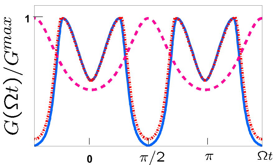
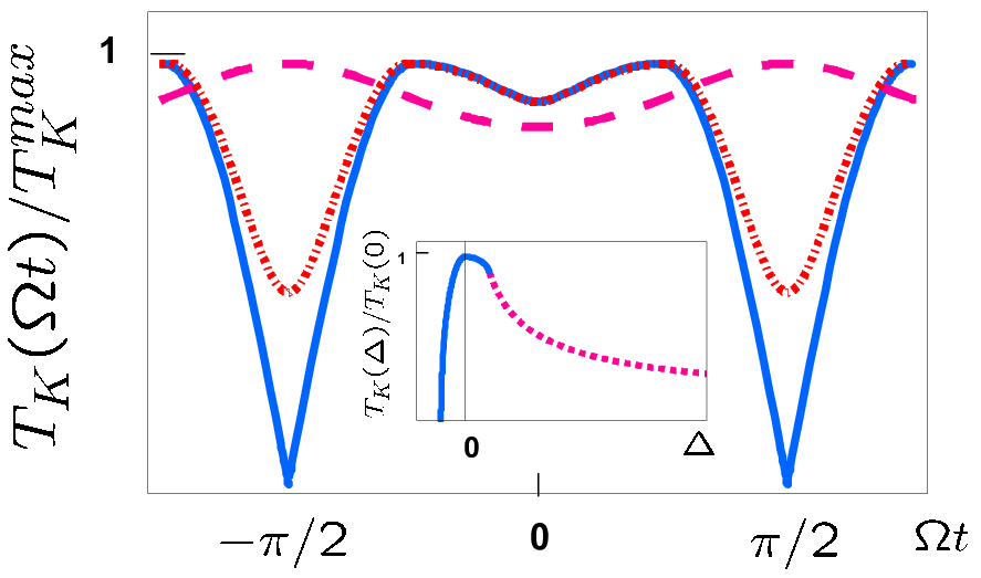
This sharp dependence is a key to the transformation mechanism of charge input into Kondo conductance response.

We estimate the influence of $\tilde{v}_{g}(t)$ on the tunnel conductance $G(T,t)$ at given $T>T_{K}$ in a situation where the adiabatic temporal variations of $T_{K}(\Delta_{ST},t)$ take place. Then the tunnel conductance obeys the law

Substituting (13) in (14), one gets

The curves $G(\Omega t)$ shown in Fig. 2 (left panel) describe transformations of an oscillating signal in the charge perturbation $\tilde{v}_{g}(t)$ into oscillations of Kondo-type zero bias anomaly (ZBA) of tunnel conductance. The transformation effect is especially distinct provided the oscillations of $v_{g}(t)$ change the sign of $\Delta_{ST}$, i.e. induce an $S\to T$ crossover (solid and dash-dotted curves in Fig. 2 corresponding to the solid part of $T_{K}(\Delta)$ curve in the inset). It is worthwhile to notice that this mechanism of the adiabatic transformation of a charge signal into Kondo response is close to the one proposed for Kondo shuttling [15] where the source of time-dependence are the nanoelectromechanical oscillations of a quantum dot.

The mechanism which converts a stochastic component $\delta v_{g}(t)$ of the input signal into a stochastic spin response is quite unusual. Instead of dephasing due to time-dependent spin flip processes [9], stochastization of the energy spectrum of DQD results in the loss of a Curie-type spin response at some characteristic energy $\zeta$. This effect is related to the time dependence of the factor $\tilde{\mu}(t)$ in the Hamiltonian (11). Indeed, inserting (9) into (11), one may write the stochastic part of $H_{\rm dot}$ as

Unlike the adiabatic part of time dependent energy levels $E_{\Lambda}(t)$ incorporated in (12), this term describes fluctuations due to the dynamical symmetry of DQD. At energies $\sim T_{K}\ll E_{E}$ the state $|E\rangle$ is frozen out. Then instead of the exact Casimir constraint (10) for the $SO(5)$ group, one deals with a fluctuating constraint ${\cal\tilde{C}}={\bf S}^{2}+{\bf P}^{2}$ for the reduced group $SO(4)$ describing an ST multiplet where the fluctuating part may be written in the form $\mu_{\rm st}(t){\bf P}^{2}=-\mu_{\rm st}(t){\bf S}^{2}$ with $\mu_{\rm st}(t)=\delta_{{\rm st},S}(t)/2$. At $T\to 0$ where the singlet is also frozen out, one arrives to the effective dot Hamiltonian

where the fermion representation for S=1, $|T\nu\rangle\langle T{\nu^{\prime}}|=f^{\dagger}_{\nu}f_{\nu^{\prime}}$, is used in the second line. Here $\varepsilon=E_{T}/2$, and the time-dependent chemical potential for spin fermions is defined as $\mu(t)=\mu_{\rm ad}-\mu_{{\rm st},S}(t)$. The stochastic component of $\mu$ may be treated as a random potential in the time domain which describes the fluctuations of the global fermionic constraint [10]. Then the propagation of spin fermions in the random time-dependent potential $\mu_{{\rm st},S}(t)$ may be studied by means of the ”cross technique” developed for the calculation of electron propagation in a field of impurities randomly distributed in real space.

The frequency $\Omega$ in $\tilde{v}_{g}(t)$ is the slowest frequency in our problem, and $\mu_{{\rm st},S}(t)$ also varies slowly in time, so that the relaxation time $\tau=\hbar/\gamma$ in the noise correlation function $D(t-t^{\prime})=\hbar^{2}\langle\mu(t)\mu(t^{\prime})\rangle\sim\exp[-\gamma(t-t^{\prime})]$ is a longest time in the model. Then one may take the limit

for its Fourier transform, $\zeta$ being the bandwidth of the Gaussian correlation. In this limit the averaged spin propagator describes the ensemble of states with chemical potential $\mu_{\rm st}$$=const$ in a given state, but this constant is random in each realization [16]. Thus the problem of decoherence of the spin state in stochastically perturbed DQD is mapped on the so-called Keldysh model [17, 18, 19] originally formulated for $\delta$-correlated impurity scattering potentials in momentum space. The problem can be solved exactly and the decoherence time is fixed by $\zeta$ of the Gaussian.

The solution of the Dyson equation obeyed by $G^{-1}(\epsilon)=\epsilon+\mu_{0}-\Sigma(\epsilon)$ (Fig. 3) [20], the Fourier transform of the spin-fermion propagator $G^{R}_{T\nu}(t-t^{\prime})=\langle f_{\nu}(t)f^{\dagger}_{\nu}(t^{\prime})\rangle_{R}=-i\langle[f_{\nu}(t)f^{\dagger}_{\nu}(t^{\prime})]_{+}\rangle$, is given by

(the index $\nu$ is omitted, since the fluctuations of $\mu$ are related to the global $U(1)$ symmetry). Using the Ward identity for a triangular vertex shown in Fig. 3, $\Gamma(\epsilon,\epsilon;0)=dG^{-1}(\epsilon)/d\epsilon$, we transform the Dyson equation into differential equation

where $x=\epsilon+\mu_{0}$ with a solution [18]

representing the set of spin states with stochastic chemical potential averaged with a gaussian exponent characterized by the dispersion $\zeta$. Remarkably, $G^{R}(x)$ has no poles, singularities or branch cuts.

To check the spin properties of stochasticized DQD, we calculate its spin response at finite $T$ determined as $\chi(i\omega_{m})=T\sum_{n}{\cal G}(i\omega_{m}+i\epsilon_{n}){\cal G}(i\epsilon_{n})\Gamma(i\epsilon_{n},i\epsilon_{n}+i\omega_{m};i\omega_{m})$ where ${\cal G}(i\epsilon_{n})$ is the Matsubara continuation of (20) on to the imaginary axis (see Fig. 3). The same Ward identity provides the exact equation for the vertex

which allows to calculate the static susceptibility

From its temperature dependence plotted in Fig. (4) we see that the the Curie-type spin response $\chi(0,T)\sim 1/T$ at high $T\gg\zeta$ transforms into a constant at zero $T$, $\chi(0,0)\sim 1/\zeta$. This means that the DQD looses at $\{\omega,T\}\ll\zeta$ the characteristics of a localized spin due stochastization, so it cannot serve as a source of Kondo screening at low energies. The frequency dependence of ${{\rm Im}\chi}(\omega,T)$ (Fig.4, inset) confirms this conclusion.

Such a behavior of the DQD affects the Kondo response described by $H_{\rm cot}$ (11). Time dependence in the vertex $\Gamma$ (Fig. 3) results in dephasing of Kondo cotunneling [10], which, however, is exponentially weak at $T\ll\Delta_{ST}$. More significant is the influence of stochastization of the DQD. Inserting (20) into the Kondo loop $K(i\epsilon_{n})\sim J^{2}T\sum_{m}\int\frac{d{\bf p}}{(2\pi)^{3}}g({\bf p},i\omega_{m}){\cal G}(i\epsilon_{n}\pm i\omega_{m})$ responsible for logarithmic singularity in conventional Kondo scattering (Fig. 3), one obtains a combination of logarithmic, hypergeometric and imaginary error functions

where $\gamma=\ln C$ is the Euler constant. In two limiting cases of low and high temperatures relative to the dispersion $\zeta$ of the noise spectrum, it leads to following expressions

Thus the noise amplitude plays the role of the infrared cut-off (similarly to Kondo-spin glass problem [21]). This cut-off distorts the coherent pulses in ZBA (Fig. 2) provided $\zeta$ is comparable with $T_{K}$ .

In conclusion, we presented and discussed the conversion mechanism of a time-dependent coherent and stochastic input signal at a gate electrode into a Kondo-type spin response in tunnel conductance. This mechanism is related to the dynamical symmetry of DQD.

Authors are indebted to F.Marquardt, N.Prokof’ev, M.V. Sadovskii and T. Ziman for valuable advices.

References

- [1] M.I. Dyakonov and V.I. Perel, Sov. Phys. JETP Lett. 13, 467 (1971).
- [2] S. Murakami, N. Nagaosa and S.-C. Zhang, Science 301, 1348 (2003); N. Sugimoto, S. Onoda, S. Murakami, and N. Nagaosa, Phys. Rev. B 73, 113305 (2006).
- [3] M.I. Dyakonov, Phys. Rev. Lett. 99, 126601 (2007).
- [4] H.-F.Lü and Y. Guo, Appl. Phys. Lett. 91, 092128 (2007)
- [5] C. Caccamo, G. Pizzimenti, and M.P. Tosi, Nuovo Cimento B31, 53 (1976).
- [6] I. D’Amico and G. Vignale, Phys. Rev. B 62, 4853 (2000).
- [7] S. Li, T.F. George, X. Sun, and L.-S. Chen, J. Phys. Chem. B 111, 6099 (2007).
- [8] K. Kikoin and Y. Avishai, Phys. Rev. Lett. 86, 2090 (2001); Phys. Rev. B 65, 115329 (2002).
- [9] A. Kaminski, Yu. V. Nazarov and L.I. Glazman, Phys. Rev. B 62, 8154 (2000).
- [10] M.N. Kiselev, K. Kikoin, Y. Avishai, and J. Richert, Phys. Rev. B 74, 115306 (2006)
- [11] F.D.M. Haldane, Phys. Rev. Lett. 40, 416 (1978).
- [12] A. Kogan, G. Granger, M.A. Kastner, D. Goldhaber-Gordon and H.Shtrikman, Phys.Rev.B67, 113309 (2003).
- [13] M. Eto and Yu.V. Nazarov, Phys. Rev. Lett. 85, 1306 (2000); M. Eto, J. Phys. Soc. Jpn, 74, 95 (2005)
- [14] M. Pustilnik and L.I. Glazman, Phys. Rev. Lett. 85, 2993 (2000), Phys. Rev. B 64, 045328 (2001).
- [15] M.N. Kiselev, K. Kikoin, R.I. Shekhter, and V.M. Vinokur, Phys. Rev. B 74, 233403 (2006).
- [16] The analog of this ensemble in real space is the inhomogeneous broadening of a ESR signal.
- [17] L.V.Keldysh, ”Semiconductors in strong electric field”, D. Sci. Thesis, Lebedev Institute, Moscow, 1965
- [18] A.Efros, Zh. Eksp. Teor. Fiz. 59, 880 (1970) [Sov. Phys.–JETP 32, 479 (1971)]
- [19] M.V.Sadovskii, ”Diagrammatica”, World Scientific, 2005
- [20] Here is a constant non-random part of .
- [21] M.N.Kiselev and R.Oppermann, JETP Lett. 71, 50 (2000) [Pisma v Zh. Eksp. Theor. Fiz. 71, 359 (2000)]