Theory of cavity-assisted microwave cooling of polar molecules.

We consider the setup shown in figure 1, where a single polar molecule is trapped close to a superconducting stripline cavity. The system Hamiltonian $H_{\rm S}$,

is given in terms of the Hamiltonian $H_{\rm c}$ for the microwave cavity, the Hamiltonian $H_{\rm m}$ describing the internal degrees of freedom of the molecule including a classical microwave driving field, as well as its motion (external degree of freedom) in the trap. Finally $H_{\rm int}$ describes the dipole interaction between rotational states of the molecule and the electric field of the cavity. Apart from the coherent evolution governed by $H_{\rm S}$, coupling of microwave photons to the electromagnetic environment introduces a dissipative decay channel for cavity photons. In section 3 we incorporate dissipation in terms of a master equation description of our system. In the following we summarize the properties of $H_{\rm S}$ which are relevant for the discussion in this paper while more details can be found in [25, 38].

With initial temperatures of the molecule in the order of 1-100 mK, electronic and vibrational degrees of freedom are frozen out and the molecule is well described by its rotational degrees of freedom only. The anharmonicity of the rotor spectrum, $E_{\rm rot}(N)=BN(N+1)$, with $B$ the rotational constant and $N$ the angular momentum quantum number, allows us to identify two specific rotational states $|g\rangle$ and $|e\rangle$ with a transition frequency $\omega_{eg}=(E_{e}-E_{g})/\hbar$ typically in the tens of GHz regime. With spontaneous emission rates of low lying rotational states in the mHz regime for zero temperature, the idea is to create an effective decay channel for the excited state $|e\rangle$ via a microwave stripline cavity. When the frequency of the relevant cavity mode $\omega_{\rm c}$ is near resonance with $\omega_{eg}$, the dynamics of the molecule is restricted to the two states $\{|g\rangle,|e\rangle\}$ and the molecule is well approximated by a two-level system (TLS).

The microwave cavity sketched in figure 1 is a (quasi-) one-dimensional superconducting stripline with length $L\sim 1$ cm, and transverse dimension of order $d\sim 1\,\mu$m. Allowed wavevectors $k_{n}=n\pi/L$ correspond to a mode spacing in the GHz regime. Restricted to a single resonator mode, the cavity Hamiltonian is $H_{\rm c}=\hbar\omega_{\rm c}c^{\dagger}c$ with $c$ ($c^{\dagger}$) the annihilation (creation) operators for photons of frequency $\omega_{\rm c}$. The electric field generated by the cavity is given by the operator $\hat{E}_{\rm c}=\mathcal{E}_{0}(\vec{r})(c+c^{\dagger})$ with $\mathcal{E}_{0}(\vec{r})$ the field strength associated with a single microwave photon. While $\mathcal{E}_{0}(\vec{r})$ varies on the scale of $L$ along the cavity axis, the spacial dependence of $\mathcal{E}_{0}(\vec{r})$ in the transverse direction or at the cavity end-caps is determined by the typical electrode spacing $d$. For strong cooling forces we are in particular interested in those strong gradients in the near field regime. The microwave photons dissipate through the coupling of the stripline to its surrounding leads. At frequencies of $\omega_{\rm c}\sim 10$ GHz, quality factors in the range of $Q\sim 10^{3}-10^{6}$ [39, 40, 41] translate into a photon loss rate $2\kappa$ in the range of MHz to kHz.

Molecules interact with microwave photons via the dipole interaction $H_{\rm int}=-\hat{\mu}\cdot\hat{E}_{\rm c}$, where $\hat{\mu}$ is the electric dipole operator of the molecule. The rotational states $|g\rangle$ and $|e\rangle$ are coupled to the quantized electric field of the cavity. Disregarding, for the moment, the motional degrees of freedom we can describe the combined cavity-molecule system, including a classical microwave field of frequency $\omega_{\rm m}$ and Rabi-frequency $\Omega$ which drives transitions between $|g\rangle$ and $|e\rangle$, by a Jaynes-Cummings type model in a frame rotating with the microwave frequency $\omega_{\rm m}$,

where $\Delta_{\rm c}=\omega_{\rm c}-\omega_{eg}$ and $\Delta=\omega_{\rm m}-\omega_{eg}$ are the detunings of the cavity field and the classical driving field from the rotational transition frequency, respectively, and we have adopted the usual Pauli operator notation for the TLS. Under resonance conditions $\omega_{c}\approx\omega_{eg}$ equation (2) describes coherent oscillations between an excitation in the TLS, $|e\rangle|n\rangle_{\rm c}$, and an additional photon in the cavity, $|g\rangle|n+1\rangle_{\rm c}$, on a timescale $(g\sqrt{n+1})^{-1}$  [42, 43]. For a molecule trapped at a distance $h\sim d\sim 1-0.1\,\mu$m above the cavity and a molecular dipole moment of the order of several Debye the vacuum Rabi frequency $g$ is of the order of $2\pi\times 50-500$ kHz [25]. In combination with this coherent energy transfer between molecule and cavity, the photon decay opens an effective decay channel for the rotationally excited state $|e\rangle$. For $\kappa>g$ the corresponding characteristic decay rate is given by

Although the validity of this expression is limited to $\gamma\lesssim g$, we find a significant increase of the rotational decay rate from $\Gamma_{eg}\sim$ mHz in free space to a cavity enhanced decay of $\gamma\sim 10-100$ kHz. This also implies that in principle cooling rates of the same order can be achieved in this system.

Trapping of a molecule close to the surface of a chip requires a sufficiently strong trapping potential; electrostatic traps with frequencies of the order of $\nu/2\pi\sim 1$ MHz are experimentally feasible [25] ¹¹ 1 In principle our derivation applies equally well to magnetic traps, as used in current atom chip experiments [44], in the case of a molecule with an unpaired electron spin. Note however that the trap fields must be compatible with the superconducting setup.. While in general the trapping potentials will be different for the two states $|g\rangle$ and $|e\rangle$, there exist so-called ‘sweet spots’ for the electric bias fields, where this difference vanishes [25]. Let us consider a 1D model in which case the external degrees of freedom are described by a harmonic oscillator Hamiltonian $H_{\rm E}=\hbar\nu a^{\dagger}a$, with $a$ ($a^{\dagger}$) the usual annihilation (creation) operators. Coupling between internal and external degrees of freedom arises from the spatial dependence of the Rabi frequencies $g\rightarrow g(\hat{x})$ and $\Omega\rightarrow\Omega(\hat{x})$, as compared to the case of laser cooling which we already remarked in the introduction. Here $\hat{x}$ is the position operator of the molecule with respect to the center of the trap. Including motional degrees of freedom into equation (2), we end up with the explicit form for the system Hamiltonian $H_{\rm S}$ (1),

The bare energy levels of $H_{\rm S}$ and the different couplings between them are sketched in figure 1 b). We emphasize at this point that the validity of $H_{\rm m}$ given in equation (4) is based on two crucial assumptions: i) the trapping potential is harmonic and ii) the trapping potential is state independent. Assumption i) is in general fulfilled near the trap center, i.e., in the final stage of the cooling process and as mentioned above, assumption ii) is fulfilled for certain conditions on the trapping fields. As neither of those assumptions will be strictly satisfied in a realistic experiment, we will investigate small deviations from these conditions in section 4. Note that as long as condition i) is approximately fulfilled we can treat the motion of the molecule along the $x$, $y$ and $z$ directions independently. This justifies the use of the one dimensional model for the motion of the molecule.

While for all cooling schemes in the optical domain the temperature of the electromagnetic environment can safely be set to zero, this assumption is in general not valid in the microwave regime. In a cryogenic environment with a temperature $T\sim 0.02-4\,K$ the thermal occupation number of the cavity mode, $N=1/[\exp(\hbar\omega_{\rm c}/k_{\rm B}T)-1]$, is typically of the order of $N\sim 0-10$. In addition to the vacuum contribution in equation (3), a finite $N$ results in cavity-assisted decay of rate $\gamma(N+1)$ and a cavity-assisted excitation rate $\gamma N$. As we discuss in more detail below, thermally activated processes are one of the limiting factors in achieving cold temperature.

When trapped close to the surface of the chip, cooling forces on the molecule arise from variations of the microwave fields on the typical length scale $d\sim 1\,\mu$m, which is only determined by the electrode geometry. For a harmonic trapping potential we compare this scale with the harmonic oscillator length $x_{0}=\sqrt{\hbar/2m\nu}$ and introduce the dimensionless parameters $\eta\equiv x_{0}\nabla\Omega/\Omega|_{x=0}$ and $\eta_{\rm c}\equiv x_{0}\nabla g/g|_{x=0}$ in analogy to the Lamb-Dicke parameter in optical cooling schemes; e.g. in the case of trapped ions, $\eta=2\pi x_{0}/\lambda$ with $\lambda$ the laser wavelength [36]. As the linear extension of the molecule trap is approximately limited by $d$ we find that cooling in this setup naturally occurs in the so-called Lamb-Dicke limit $\eta,\eta_{\rm c}\approx x_{0}/d\ll 1$, where the spatial extension of the molecule wavepacket is small compared to variations of the microwave fields. While typically $\eta$ and $\eta_{\rm c}$ will be equal or at least of the same order, in the following discussion we treat them as two independent parameters.

In the Lamb-Dicke limit we can expand the Hamiltonian (4) to first order in $\hat{x}$, i.e. $H_{\rm S}\simeq H_{0}+H_{1}$. Here $H_{0}$ is the Hamiltonian describing the free evolution of the internal and motional degrees of freedom of the molecule. The coupling between the internal and motional degrees of freedom is of the form

such that $\langle\hat{F}\rangle$ is the mean dipole force exerted on the molecule. The small parameters $\eta$ and $\eta_{\rm c}$ allow us to treat $H_{1}$ as a weak perturbation for the decoupled dynamics of the system. For $|H_{1}|\ll\Gamma_{\rm I}$, with $\Gamma_{\rm I}={\rm min}\{\gamma,\kappa\}$ the characteristic relaxation rate of the cavity-molecule system, we can adiabatically eliminate the internal degrees of freedom (see section 3) and derive an effective equation of motion for the reduced external density operator $\mu(t)$. The resulting equation for the mean occupation number $\langle n\rangle(t)={\rm Tr}\{a^{\dagger}a\mu(t)\}$ (see also [29, 36, 45]) is of the form

For a positive damping rate $W>0$, equation (6) describes relaxation of the mean occupation number to a final steady state value $\langle n\rangle_{0}$. The relevant quantities characterizing the cooling dynamics, $W$ and $\langle n\rangle_{0}$, are given by

where the cooling and heating rates $A_{-}=S(\nu)$ and $A_{+}=S(-\nu)$ are determined by the spectrum of the force operator,

Equations (6)-(8) provide the general relation between the cooling dynamics of the external degrees of freedom and the fluctuation spectrum of the internal operator $\hat{F}$. Efficient cooling schemes correspond to the case where both the difference $S(\nu)-S(-\nu)$ is maximized (large cooling rate) and the ratio $S(-\nu)/S(\nu)$ is minimized (low final temperatures). Throughout this paper we make extensive use of this relation to discuss different cooling schemes in terms of the properties of $S(\omega)$.

While the results for cooling in the Lamb-Dicke limit summarized in equations (6)-(8) are valid for arbitrary cavity-molecule interactions, we concentrate in the remainder of this paper on the bad cavity limit (BCL), $g\ll\kappa$, which we expect to be the most relevant regime in experiments. For additional discussions on cavity cooling of atoms in the good cavity limit the reader is referred to [29].

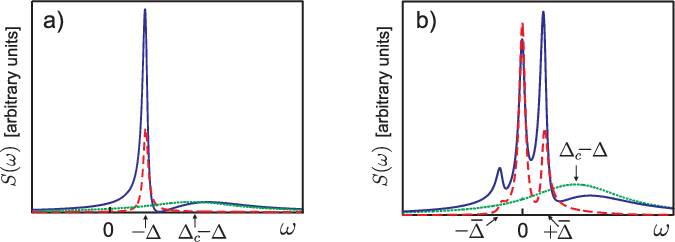
The BCL allows us to eliminate the cavity degrees of freedom and to study and interpret cavity-cooling in terms of the resulting effective dynamics for the molecule. However, based on the underlying coherent interaction and the finite bandwidth of the cavity mode, the effective dynamics of the molecule differs significantly from the usual case of a two level atom coupled to the free radiation field. The adiabatic elimination of the cavity mode, which is discussed in more detail in section 3, results in a decomposition of the general form of $S(\omega)$ given in equation (8) into three contributions,

The labels on the first two terms refer to their origin; the spectrum $S_{\Omega}$ is associated with the force from the drive field gradient $\nabla\Omega$ and exhibits sharp resonances of width $\sim\gamma$, whereas $S_{g}$ is associated with the force due to the cavity-TLS coupling gradient, $\nabla g$, and exhibits a broader resonance of width $2\kappa$. As explained in more detail in the following discussion, we can with each of these forces associate a different cooling mechanism in our system. The third contribution to the spectrum, $S_{I}$, describes destructive and constructive interference between the different cooling processes. For illustration, the spectrum $S(\omega)$ and its decomposition according to equation (9) are shown in figure 2 for the case of zero temperature and a) for a weakly ($\Omega\ll|\Delta|$) and b) for a strongly ($\Omega\sim|\Delta|$) driven molecule.

The results presented in this overview section apply to a weakly driven molecule, and generalizations to arbitrary $\Omega$ are derived in section 4.

For the elimination of the cavity degrees of freedom we decompose the total Liouville operator $\mathcal{L}$ defined in equation (15) into three contributions

The first two terms describe the uncoupled dynamics of the cavity mode,

and the molecular degrees of freedom,

whereas the interaction between the cavity mode and the molecule is described by the last term in equation (17),

In the decoupled limit $g\rightarrow 0$ the cavity field evolves independently of the molecule. On a timescale $\kappa^{-1}$ the system relaxes into the state $\rho(t)\approx\rho^{0}_{\rm c}\otimes\rho_{\rm m}(t)$, with $\rho_{\rm c}^{0}$ the cavity equilibrium density operator defined by $\mathcal{L}_{\rm c}(\rho_{\rm c}^{0})=0$, and the molecular operator $\rho_{\rm m}(t)$ evolving under the action of $\mathcal{L}_{\rm m}$. For a finite coupling $g\ll\kappa$ deviations from the factorized form of $\rho(t)$ are small, but the coupling term $\mathcal{L}_{g}$ modifies the dynamics of $\rho_{\rm m}(t)$. To proceed we adopt a projection operator technique along the lines of reference [45] and define the projector $\mathcal{P}\rho=\rho_{\rm c}^{0}\otimes{\rm Tr}_{\rm c}\{\rho\}$ and its orthogonal complement $\mathcal{Q}=(1-\mathcal{P})$. Inserting the decomposition $\rho(t)=\mathcal{P}\rho(t)+\mathcal{Q}\rho(t)$ into equation (15) we obtain the two coupled equations

As the population in the subspace $\mathcal{Q}\rho$ is damped with a rate $\kappa$ which is fast compared to the coupling term $\mathcal{Q}\mathcal{L}_{g}\mathcal{P}\sim g$, we formally integrate equation (22), insert the result into equation (21) and expand the final expression up to second order in $g$. For times $t\gg\kappa^{-1}$ we end up with an effective master equation for the molecule density operator $\rho_{\rm m}(t)={\rm Tr}_{\rm c}\{\mathcal{P}\rho(t)\}$ which is given by

Strictly speaking the effective master equation (23) is valid in the limit $g\sqrt{N+1}/\kappa\ll 1$, but we expect it to hold to a good approximation also for a slightly relaxed condition, $g\lesssim\kappa$.

The second term in equation (23) describes the effect of the cavity on the molecular dynamics. We evaluate this term by inserting the definitions of $\mathcal{L}_{\rm c}$, $\mathcal{L}_{\rm m}$ and $\mathcal{L}_{g}$ given in equations (18)-(20) and obtain an effective master equation on the form (see also [45])

Here we introduced the abbreviations $S=g(\hat{x})\sigma_{-}$ and

In summary we have derived an effective master equation (24) for the molecule, where the first term describes the bare evolution, and the second term describes the influence of the cavity on the dynamics. We want to point out that the latter term in general has a complicated form, since the operator $T$ (25) depends on the bare molecule Hamiltonian $H_{\rm m}$. Only in the infinite bandwidth limit, where $\kappa$ is large compared to $\Delta,\Omega$ and $\nu$, will equation (25) reduce to the simple form $T=S/(\kappa-i\Delta_{\rm c})$.

To proceed with the derivation, we now consider the master equation (24) in the Lamb-Dicke limit $\eta,\eta_{\rm c}\ll 1$ where internal and external degrees of freedom interact weakly. We expand the position dependent Rabi frequencies $\Omega(\hat{x})$ and $g(\hat{x})$ up to first order in the Lamb-Dicke parameters, i.e.,

Under the same approximation the operator $T$ gets the form

with $\Sigma_{-}(\nu),\Sigma_{+}(\nu)=\Sigma_{-}^{\dagger}(-\nu)$ effective TLS operators defined in (59). Up to second order in the Lamb-Dicke parameters we obtain the master equation

where the subscripts indicate the respective order in the Lamb-Dicke parameters $\eta,\eta_{\rm c}$. The zeroth order term is given by

where $\mathcal{L}_{\rm E}(\rho)=-i\nu[a^{\dagger}a,\rho]$ describes the uncoupled external dynamics of the molecule, and $\mathcal{L}_{\rm I}$ describes the effective dynamics of the uncoupled TLS,

Explicit expressions for $\mathcal{L}_{1}$ and $\mathcal{L}_{2}$ are listed in A. Let us for the moment consider the effective dynamics of the TLS (30), with the corresponding Bloch equations for the set of operators $\{\sigma_{x},\sigma_{y},\sigma_{z}\}$ of the form

Here $\tilde{\gamma}_{N}=(2N+1)\tilde{\gamma}$ and the remaining parameters are defined in B. In the discussion in section 4 we will mainly focus on the limit $\Omega\ll\kappa$ where the parameters $\delta_{x,y},\gamma_{x,y},\Omega_{x,y}$ and $\Gamma_{x,y}$ are small and equation (31) reduces to the normal Bloch equations for a two level system coupled to a thermal bath. Further the stark shift $\tilde{\delta}$ and the effective decay rate $\tilde{\gamma}$ reduce to the familiar expressions

For the purpose of readability, we will use the simplification $\Delta+\tilde{\delta}\rightarrow\Delta$ in the following. Finally note that when the driving strength $\Omega$ is comparable to the cavity linewidth $\kappa$, unless $|\Delta|,|\Delta_{\rm c}|\gg\kappa$ there will be modifications of $\delta$ and $\gamma$. In addition, the non-standard terms in the Bloch equations (31) introduce new features in the TLS dynamics which modify the force spectrum $S(\omega)$ and in the end the cooling dynamics. A detailed discussion of the effective dynamics of a strongly driven TLS inside a cavity is given in [48].

Starting from equation (28) we further eliminate the internal degrees of freedom in a similar fashion as the above elimination of the cavity mode, following the procedure in [45]. First we notice that the zeroth order term ${\mathcal{L}}_{0}$ in the expansion (28) describes the uncoupled dynamics of the internal and external degrees of freedom, whereas the higher order terms ${\mathcal{L}}_{1,2}$ couple the external and internal dynamics and therefore introduce forces acting on the molecule motion. Provided the coupling is weak compared to the energy scales defining the TLS dynamics, $\eta\Omega,\eta_{\rm c}g^{2}/\kappa\ll\gamma_{N}$, the state of the TLS will deviate only slightly from the equilibrium state due to the interaction, and the dynamics of the TLS can be eliminated. We define a projection operator $\mathcal{P}_{\mu}$,

with $\rho_{\rm I}^{0}$ the internal equilibrium state defined by $\mathcal{L}_{0}(\rho_{\rm I}^{0})=0$. Second order perturbation theory in the Lamb-Dicke parameters $\eta,\eta_{\rm c}\ll 1$ results in a master equation for the external operator $\mu(t)={\rm Tr}_{\rm I}\{\mathcal{P}_{\mu}\rho_{\rm m}(t)\}$, which describes the evolution of the population of the individual trap levels. We obtain

Inserting the definitions of $\mathcal{L}_{1,2}$ given in A we end up with a master equation on the form

and recover the cooling equation (6) given in section 2 with $W=(A_{-}-A_{+})$ and $\langle n\rangle_{0}=A_{+}/W$. The heating and cooling coefficients $A_{\pm}$ which follow from an evaluation of equation (34) can be divided into three contributions,

where the physical motivation for the decomposition (36) has been presented in section 2. The first contribution to the force spectrum, $S_{\Omega}(\omega)$, follows from the first term of equation (34) in the limit $\eta_{\rm c}\rightarrow 0$ and is defined as

The second term, $S_{g}(\omega)$, follows from the second term in equation (34) and is given by

with effective TLS operators $\Sigma_{\pm}(\nu)$ given by (61). Finally, remaining contributions from the first term in equation (34) are found by making the Ansatz,

The result is summarized by $S_{I}(\omega)$ defined as

with the action of the superoperators $\mathcal{K}_{\pm}$ given by

In conclusion, we have expressed heating and cooling rates $A_{\pm}$ in terms of two-point correlation functions and steady state expectation values of a TLS whose evolution is described in terms of the effective Bloch equations (31). The results are valid for $g\sqrt{N+1}\ll\kappa$ and $\eta\Omega\ll\gamma_{N}$, $\eta_{\rm c}\ll 1$ but at this stage no further assumptions have been made. However, in the following we mainly concentrate on the case $\Omega\ll\kappa$ or on the regime $\Omega\sim\kappa$, $|\Delta_{\rm c}|,|\Delta|\gg\Omega$ where the Bloch equations reduce to the standard form (see B). Using the quantum regression theorem and the steady state solution of equation (31) we outline the derivation of analytic expressions for $S_{\Omega}(\omega)$ and $S_{g}(\omega)$ in C and D. Analytic expressions for $S_{I}(\omega)$ could in principle be derived along the same lines but in general do not have simple enough form to provide further insight. Therefore we will rather use numerical calculations in combination with previously derived results for the weak excitation limit [29] as a basis for the discussion of the interference terms.

We start the discussion with the mechanism of cavity assisted sideband cooling (CASC) where the corresponding cooling rate $W_{\Omega}=S_{\Omega}(\nu)-S_{\Omega}(-\nu)$ and steady state occupation $\langle n\rangle_{0,\Omega}=S_{\Omega}(-\nu)/W_{\Omega}$ depend on the spectrum $S_{\Omega}(\omega)$ defined in equation (37). Following the calculations outlined in C we obtain for the spectrum in the weak driving limit, $\Omega\ll\gamma_{N}$,

For a fixed ratio $\nu/\gamma_{N}$ we optimize $\langle n\rangle_{0,\Omega}$ with respect to the detuning $\Delta$, where obviously $\Delta$ must be negative to promote cooling. For the two limits of interest, the resolved sideband limit (SB) $\nu\gg\gamma_{N}$ and the Doppler limit (D) $\nu\ll\gamma_{N}$, we find $\Delta=-\nu$ and $\Delta=-\gamma_{N}/2$ respectively. The final occupation number is given by the respective expressions (10) and (11) in section 2, and the corresponding cooling rates are given by,

Although in the weak driving limit the final occupation number is independent of $\Omega$, the cooling rate scales as $W_{\Omega}\sim\Omega^{2}$ and under the validity of equation (43) it is bounded be $W_{\Omega}<\eta^{2}\gamma$. In competition with the cavity-mediated thermalization process of the molecule, discussed in section 2, it is therefore necessary to study sideband cooling beyond the weak driving regime.

Let us now consider an arbitrary $\Omega$, but focus on CASC in the sideband resolved limit $\gamma_{N}/\nu\ll 1$. As shown in C, the spectrum now exhibits a three-peak structure and reads,

with $\bar{\Delta}=\sqrt{\Omega^{2}+\Delta^{2}}$. For sideband cooling we are only interested in the peaks at nonzero frequency. The relative heights of the resonances, $\alpha_{\pm}$, and the widths $\bar{\gamma},\bar{\gamma}_{0}$ which are proportional to $\gamma_{N}$ are defined in C and are functions of $\Omega$, $\Delta$ and $N$. For $W_{\Omega}$ to be positive we require a red detuned microwave field $\Delta<0$ and cooling is optimized for $\nu=\bar{\Delta}$. Under those conditions we obtain

with ${\rm g}(\varphi)=4\sin^{2}\varphi|\cos^{3}\varphi|/(4-\sin^{4}\varphi)$, and

References

- [1] See e.g. Special Issue: Ultracold Polar Molecules: Formation and Collisions 2004 Eur. Phys. J. D 31 149-445
- [2] Krems R V 2005 Int. Rev. Phys. Chem. 24 99, and references therein.
- [3] Hudson J J, Sauer B E, Tarbutt M R and Hinds E A 2002 Phys. Rev. Lett. 89 023003
- [4] DeMille D, Cahn S B, Murphree D, Rahmlow D A and Kozlov M G 2008 Phys. Rev. Lett. 100 023003
- [5] DeMille D 2002 Phys. Rev. Lett. 88 067901
- [6] Yelin S F, Kirby K and Côté R 2006 Phys. Rev.A 74 050301(R)
- [7] Wang D, Lukin M D and Demler E 2006 Phys. Rev. Lett. 97 180413
- [8] Micheli A, Brennen G K and Zoller P 2006 Nature Physics 2 341
- [9] Büchler H P, Micheli A and Zoller P 2007 Nature Physics 3 726
- [10] For a review on experimental progress in the field of cold molecules see Doyle J, Friedrich B, Krems R V and Masnou-Seeuws F 2004 Eur. Phys. J. D 31 149, and references cited.
- [11] Vuletić V, Chan H W and Black A T 2001 Phys. Rev.A 64 033405
- [12] Morigi G, Pinkse P W, Kowalewski M and de Vivie-Riedle R 2007 Phys. Rev. Lett. 99 073001
- [13] Lev B L, Vukics A, Hudson E R, Sawyer B C, Domokos P, Ritsch H and Ye J 2008 Phys. Rev.A 77 023402
- [14] van de Meerakker S Y T, Vanhaecke N and Meijer G 2006 Annual Review of Physical Chemistry 57 159
- [15] Campbell W C, Tsikata E, Lu H I, van Buuren L D and Doyle J M 2007 Phys. Rev. Lett. 98 213001
- [16] Tarbutt M R, Bethlem H L, Hudson J J, Ryabov V L, Ryzhov V A, Sauer B E, Meijer G and Hinds E A 2004 Phys. Rev. Lett. 92 173002
- [17] Rieger T, Junglen T, Rangwala S A, Pinkse P W H and Rempe G 2005 Phys. Rev. Lett. 95 173002
- [18] Meek S A, Bethlem H L, Conrad H, Meijer G 2008 Preprint arXiv:0801.2943
- [19] Avdeenkov A V, Kajita M and Bohn J L 2006 Phys. Rev.A 73 022707
- [20] Lara M, Bohn J L, Potter D, Soldán P and Hutson J M 2006 Phys. Rev. Lett. 97 183201
- [21] Mancini M W, Telles G D, Caires A R L, Bagnato V S and Marcassa L G 2004 Phys. Rev. Lett. 92 133203
- [22] Sage J M, Sainis S, Bergeman T and DeMille D 2005 Phys. Rev. Lett. 94 203001
- [23] Wang D, Qi J, Stone M F, Nikolayeva O, Wang H, Hattaway B, Gensemer S D, Gould P L, Eyler E E and Stwalley W C 2004 Phys. Rev. Lett. 93 243005
- [24] Kleinert J, Haimberger C, Zabawa P J and Bigelow N P 2007 Phys. Rev. Lett. 99 143002
- [25] Andre A, DeMille D, Doyle J M, Lukin M D, Maxwell S E, Rabl P, Schoelkopf R and Zoller P 2006 Nature Physics 2 636
- [26] Cirac J I, Lewenstein M and Zoller P 1995 Phys. Rev.A 51 1650
- [27] Horak P, Hechenblaikner G, Gheri K M, Stecher H and Ritsch H 1997 Phys. Rev. Lett. 79 4974
- [28] Zippilli S and Morigi G 2005 Phys. Rev. Lett. 95 143001
- [29] Zippilli S and Morigi G 2005 Phys. Rev.A 72 053408
- [30] Maunz P, Puppe T, Schuster I, Syassen N, Pinkse P W H, and Rempe G 2004 Nature 428 50
- [31] Boozer A D, Boca A, Miller R, Northup T E and Kimble H J 2006 Phys. Rev. Lett. 97 083602
- [32] Tscherbul T V and Krems R V 2006 Phys. Rev. Lett. 97 083201
- [33] Krems R V and Dalgarno A 2004 J. Chem. Phys. 120 2296
- [34] Ticknor C and Bohn J L 2005 Phys. Rev.A 72 032717
- [35] Rabl P, DeMille D, Doyle J M, Lukin M D, Schoelkopf R J and Zoller P 2006 Phys. Rev. Lett. 97 033003
- [36] Stenholm S 1986 Rev. Mod. Phys. 58 699
- [37] Leibfried D, Blatt R, Monroe C and Wineland D 2003 Rev. Mod. Phys. 75 281
- [38] Rabl P and Zoller P 2007 Phys. Rev.A 76 042308
- [39] Day P K, LeDuc H G, Mazin B A, Vayonakis A and Zmuidzinas J 2003 Nature 425 817
- [40] Wallraff A, Schuster D I, Blais A, Frunzio L, Huang R-S, Majer J, Kumar S, Girvin S M and Schoelkopf R J 2004 Nature 431 162
- [41] Frunzio L, Wallraff A, Schuster D, Majer J and Schoelkopf R 2005 IEEE Trans. Appl. Supercond. 15 860
- [42] Hood C J, Lynn T W, Doherty A C, Parkins A S and Kimble H J 2000 Science 287 1447
- [43] Raimond J M, Brune M and Haroche S 2001 Rev. Mod. Phys. 73 565
- [44] See, for example, Fortágh J and Zimmermann C 2007 Rev. Mod. Phys. 79 235 and references therein.
- [45] Cirac J I, Blatt R, Zoller P and Phillips W D 1992 Phys. Rev.A 46 2668
- [46] Morigi G, Eschner J and Keitel C H 2000 Phys. Rev. Lett. 85 4458
- [47] Roos C F, Leibfried D, Mundt A, Schmidt-Kaler F, Eschner J and Blatt R 2000 Phys. Rev. Lett. 85 5547
- [48] Cirac J I, Ritsch H and Zoller P 1991 Phys. Rev.A 44 4541
- [49] Walls D F and Milburn G J 1994 Quantum Optics (Springer-Verlag Berlin).
- [50] Wallquist M, Shumeiko V S and Wendin G 2006 Phys. Rev.B 74 224506
- [51] Sandberg M, Wilson C M, Person F, Johansson G, Shumeiko V S, Duty T and Delsing P 2008 Preprint arXiv:0801.2479
- [52] Palacios-Laloy A, Nguyen F, Mallet F, Bertet P, Vion D and Esteve D 2007 Preprint arXiv:0712.0221