Discontinuity of the chemical potential in RDMFT for open-shell systems
Abstract
We employ reduced density-matrix functional theory in the calculation of the fundamental gap of open-shell systems. The formula for the calculation of the fundamental gap is derived with special attention to the spin of the neutral and the charged systems. We discuss the effects of different functionals as well as the changes due to different basis sets. Also, we investigate the importance of varying the natural orbitals for the calculation of the fundamental gap.
I Introduction
Density functional theory (DFT) [1, 2] is a powerful tool to calculate the electronic structure of atoms, molecules, and solids. Within DFT observables are given as functionals of the particle density. In reduced density-matrix functional theory (RDMFT) the 1-body reduced density matrix (1-RDM) is used as the basic variable. RDMFT is based on Gilbert’s theorem [3] which proves that each ground-state observable can, in principle, be written as a functional of the 1-RDM. First-generation functionals [4, 6, 5] perform very well in the description of the dissociation of small molecules. Second generation functionals were introduced very recently [7, 8, 9] which improved both the performance for small molecules [7, 8, 9] and also for the homogeneous electron gas [10].
A key quantity in electronic structure calculations is the band gap for semiconductors and insulators. It is defined as the difference between the ionization potential and the electron affinity
| (1) |
where
| (2) | |||||
| (3) |
denotes the ground-state energy of an -electron system. In the chemistry literature is called the chemical hardness if the system is finite. For simplicity we use the term fundamental gap for both finite and extended systems throughout this article. We like to point out that the fundamental gap differs from what is known as the optical gap. The optical gap is given as the energy necessary to excite the system from the ground state to the first excited state. Therefore, its size is reduced by the binding energy of the created exciton compared to the fundamental gap.
Within density functional theory it can be shown [11, 12] that the fundamental gap is exactly given by
| (4) |
where is the energy difference between the lowest unoccupied and the highest occupied Kohn-Sham states and is the discontinuity of the exchange-correlation potential upon adding and subtracting a fractional charge. This discontinuity is zero for LDA and GGA, so is the prediction for the gap within these approximations. However, this prediction deviates strongly from the experimental values. For semiconductors the calculated gap underestimates the experimental value by typically 50%. In extreme cases, such as germanium, the gap vanishes within LDA. Interestingly, for the exact-exchange functional is very close to the experimental gap for several systems [13, 14]. Unfortunately, in the case of exact exchange is not zero and, in fact, was found to be much larger than . Thus, if properly calculated, the band gaps within exact exchange are highly overestimated compared to the experimental values [13, 14, 15, 16]. Exact exchange combined with RPA correlation was recently shown to yield results very close to the experimental values for Si, LiF, and solid Ar [16] (provided the discontinuity is properly included). Finally, a recently introduced hybrid functional (HSE) [17, 18] is reported to give gaps in satisfactory agreement with experimental values for a set of 40 simple and binary semiconductors [19]. Especially, germanium is predicted a semiconductor with a gap of 0.56 eV.
An alternative formula to (4) for the fundamental gap in DFT reads [20]
| (5) |
where is the chemical potential, and is the particle number of the system. As Eq. (5) suggests, the chemical potential has a discontinuity at integer particle number . In a recent paper [26], we presented the analogous equation within reduced density-matrix functional theory. In particular, we proved that the Lagrange multiplier used to enforce the conservation of particle number is equal to the chemical potential. This theoretical development was applied to small finite and prototype periodic systems with very promising results. We like to emphasize that the analogy between DFT and RDMFT is not at all trivial because of the -representability condition in RDMFT. The occupation numbers are restricted to the interval which leads to border minima. For this reason the generalization of the proof of Eq. (5) from DFT to RDMFT is not straightforward.
In the present work, we deduce a relationship similar to Eq. (5) for open-shell systems. The difficulty in generalizing Eq. (5) to the open-shell case arizes from the fact that adding/subracting a spin-up electron to/from an open-shell ground state is not equivalent to adding/subtracting a spin-down electron. Open-shell systems were recently addressed in Ref. 21 where it was demonstrated that it is reasonable to introduce two Lagrange multipliers to keep the number of electrons in each spin channel fixed seperately. An alternative description of open-shell systems was introduced by Leiva and Piris [22]. In that desription, however, spin-up and spin-down occupations are equal for all orbitals except the open-shell ones which are fully occupied by the majority spin. The Lagrange multiplier is then spin independent. Here, we employ the treatment suggested in Ref. 21 where each of the two Lagrange multipliers is a function of the two particle numbers corresponding to the two spin components. In the present work, these particle numbers are assumed to be fractional. We show that a proper extension of Eq. (5) is possible with the resulting equation involving the discontinuities of both Lagrange multipliers. The derivation is presented in Section II. Section III contains results for a set of open-shell atoms and a comparison of the closed- and open-shell treatment for systems where the neutral system is actually closed-shell. We also investigate the performance of different functionals in the calculation of the fundamental gap.
II The fundamental gap in RDMFT
Reduced-density-matrix-functional theory (RDMFT) uses the one-body reduced density matrix (1-RDM)
| (6) |
where denotes the many-body wave function and . Integration over means integration over space and summation over spin. Throughout this article we restrict ourselves, for simplicity, to the ”collinear” case where is diagonal in spin space, i.e.
| (7) |
By diagonalizing one obtains the natural orbitals and the occupation numbers , i.e.
| (8) |
To ensure the -representability of the occupation numbers are restricted to the interval and sum up to the total number of particles . In closed-shell systems the two spin-directions are identical, i.e.
| (9) | |||||
| (10) |
Within the spin-dependent formalism one can define spin-dependent electron affinities and ionization potentials by adding or removing an electron with specific spin
| (11) | |||||
| (12) |
Here, representes the ground-state energy of a system with electrons where is the number of electrons with spin and is the number of electrons with the opposite spin, . Consequently, the ionization potential and electron affinity defined in Eq. (3) are given by
| (13) | |||
| (14) |
i.e. they are respectively the smallest necessary energy for taking away an electron and the maximum energy gained by adding an electron to the neutral system. The fundamental gap then reads
| (15) |
In order to derive a formula analogous to Eq. (5) for the fundamental gap (1) within RDMFT we follow the same path as in DFT [23, 12, 24] and extend the definition of the total-energy functional to systems with fractional particle number . Throughout this paper we use the convention that denotes an integer number of particles and a fractional. Such systems can be described as an ensemble consisting of an - and an -particle state for . Let denote an -particle wave function with where, as before, is the number of electrons with spin and the number of particles with the opposite spin, . We consider an ensemble where, compared to the charge-neutral system, the number of spin- particles is increased by . The statistical operator describing such an ensemble is given by
| (16) |
The expectation value of an operator is then given by
| (17) |
In particular, for , i.e. the operator representing the 1-RDM of spin- particles, we obtain
| (18) |
and for , i.e. the Hamiltonian, we get the total ensemble energy
| (19) |
We note in passing that the ensemble weights in Eq. (16) are such that the correct normalization of spin-up and spin-down densities is achieved, i.e.
| (20) | |||||
| (21) |
Reformulating (19) one obtains
| (22) |
for . In analogy, for the total energy is given by
| (23) |
In other words, the total energy depends linearly on with slope for and slope for . Since and are in general not the same, the derivative has a discontinuity at integer particle number . From Eqs. (11)-(15), one can conclude that the fundamental gap is given by
| (24) |
In Ref 21, we argued that, for open-shell systems, the following functional should be minimized
| (25) |
The Lagrange multipliers and are introduced to achieve given particle numbers and . To prove the formula for the fundamental gap we first show that these Lagrange multipliers are nothing but the chemical potentials, i.e.
| (26) |
The derivation of this formula differs significantly from the derivation of its counterpart in DFT due to the above mentioned -representability constraint. In order for the 1-RDM to be connected to an anti-symmetric -particle wave function its occupation numbers have to be restricted to the interval [0,1] [25]. One can show that the same constraint ensures ensemble -representability for fractional particle number. As a result of this additional constraint, need not vanish at the minimum energy. It is possible that certain occupation numbers are pinned at the border of the interval while the true minimum is obtained for values of outside this interval. The functional then has a border minimum, and therefore non-vanishing derivative, in all directions where occupation numbers are pinned at zero or one.
We investigate the difference
| (27) |
A Taylor expansion of around yields
| (28) |
For the functional derivative we employ (25) and obtain
| (29) |
The first term on the right is evaluated via the functional chain rule, i.e.
| (30) |
At the solution point, the variation with respect to the natural orbitals vanishes such that the second term on the right is zero. The variation with respect to the occupation numbers, however, need not vanish due to the -representability constraint. Equation (28) therefore reduces to
| (31) |
where the first sum runs only over those occupation numbers pinned to the border of the interval. The variation of the occupation numbers can be calculated applying first order perturbation theory to the eigenvalue equation of the 1-RDM
| (32) |
which yields
| (33) |
In addition, we write the eigenvalues and eigenfunctions of as
| (34) |
where and denote the natural orbitals and occupation numbers of . Equation (31) then reduces to
| (35) | |||||
where we only kept terms up to first order. In order for the natural orbitals to remain normalized the changes have to be orthogonal to the original orbitals, i.e.
| (36) |
Therefore, the integrals one the right-hand-side of Eq. (35) vanish. The sum over all changes in the occupation numbers has to give in order for the new occupation numbers to sum up to the correct particle number. Hence, we obtain
| (37) |
Finally, we discuss the contribution of the pinned states. As stated before, for these states is different from zero and the true minimum of the functional lies outside the interval [0,1]. More specifically, it lies at a finite distance from the border of the interval such that the addition or subtraction of an infinitesimal fraction of a particle cannot move the minimum into the interval. Therefore, these particle numbers remain pinned upon adding or subtracting an infinitesimal , i.e. is zero in the limit . We therefore conclude
| (38) | |||||
Using Equation (24) we obtain the final result for the fundamental gap
| (39) |
The derivation of Eq. (39) concerns the exact exchange-correlation energy functional of the 1-RDM. Since only approximations are available, the question is whether Eq. (39) is still useful. This question is the main subject of the next section.
In Ref. 26, a single, spin independent (for closed-shell systems) was shown to have a discontinuity as a function of a fractional total number of electrons which is equally distributed in the two spin channels. The application of that theory to an open-shell system would give the spin resolved as a function of a unique . In the present work, we add/subtract a fractional part of an electron to/from a specific spin channel. Consequently, the system becomes an open-shell system even if the neutral system is closed-shell. Thus, we have four functions , , , and , where , are fixed to the integer values of the neutral system. Of these four, only the first two show a discontinuity. The correct gap is then given by Eq. (39), where the min and max functions take care of the selection of the smallest ionization potential and the largest electron affinity. Alternatively, one can employ Eqs. (1)-(3) for the calculation of the fundamental gap. Both approaches are exact, in the sense that, given the exact functional of , they both reproduce the fundamental gap. It is interesting to see if they give the same numbers for approximate functionals as well. This is also one of the questions we address in the next section.
To answer the above questions, one needs to minimize the approximate functionals for fractional number of particles to get . The extension of the minimization procedure to fractional particle numbers, which is in complete accordance with the proof we presented above, requires us to perform the minimization in the domain of , which are given by Eq. (18). In principle one then has to minimize the total energy with respect to and under the known -representability constraints that their occupation numbers are between 0 and 1 and sum up to the correct particle numbers. However, this procedure, involving the density matrices for and particles, is not very practical. On the contrary, it is desirable to minimize with respect to directly under the appropriate constraints. We prove elsewhere [27] that the appropriate constraints for such a minimization are
| (40) |
In other words, the domain of which can be represented as the weighted average Eq. (18) is identical to the domain of whose eigenvalues satisfy Eq. (40). The above statement is quite significant since the constraint of Eq. (40) is much simpler and completely analogous to the case of integer particle numbers. The implementation is therefore a rather simple extension of the case of integer particle numbers.
III Numerical results
In this section, we study the behavior of as a function of the fractional particle number for some atoms and molecules using approximate functionals of the 1-RDM. Our aim is to investigate whether there exists a discontinuity in and how it compares to the fundamental gap. The implementation we used for finite systems can be applied to both closed- and open-shell [21] configurations. Some results for closed-shell systems were presented in Ref. 26. Here, we give an extended analysis for both closed- and open-shell systems.
For the open-shell treatment, we use the extension of the functional of Goedecker-Umrigar[5] described in Ref. 21. We also investigate whether other functionals reproduce a discontinuity in a closed-shell treatment. For this purpose we consider the functionals of Piris[8, 9], where the self-interaction (SI) terms are explicitly removed, and the Müller functional and the most recent BBC functionals of Gritsenko et al[7] which contain self-interaction terms.
The implementation is based on the GAMESS program[28] which we use for the calculation of the one and two-electron integrals. The minimization with respect to the occupation numbers and natural orbitals is then performed using the conjugate gradient method. Our program treats both closed- as well as open-shell systems using the restricted open-shell RDMFT [21]. In short, we assume spin-dependent occupation numbers (and chemical potentials) but spin-independent natural orbitals. In that way, our method is in complete analogy to spin restricted open-shell Hartree-Fock.


In Fig. 1a, we show for the LiH molecule using the GU functional in the closed-shell treatment, i.e. the extra charge is equally distributed over the two spin channels. Fig. 1b shows and for the open-shell treatment of the LiH molecule, using again the GU functional. In the open-shell treatment the additional charge is exclusively added to one spin channel, and here we choose the spin-up channel. Clearly, in Fig. 1a and in Fig. 1b show a pronounced step which resembles the discontinuity that one expects for the exact functional. This step has two important features: the first is that it occurs not exactly at , i.e. the exact, integer number of electrons. It is rather shifted slightly to the right. The shift is of the order of 0.05 of an electron in Fig. 1a and is reduced to 0.02 in Fig. 1b. A closer look at the solution reveals that the bottom of the step appears exactly at the point where the occupation number of the HOMO gets equal to one. After that point it has to remain one due to the -representability constraints, Eq. (40). The pinning of the occupation number of the HOMO to one results in the rapid increase of . Since adding charge to one spin channel only results in faster pinning of the HOMO state it is not surprising that the step in the open-shell treatment is shifted to the left. Upon increasing the extra charge further, is a smooth function, i.e. the upper edge of the step is rounded off. In the closed-shell treatment shows a linear dependence outside the step region, which is significantly reduced in in closer resemblance to the exact behavior. A more detailed investigation reveals that the slope of is the average of the slopes of and . To extract a value for the discontinuity we use a backwards projection as shown in Fig. 1. This method reduces to the exact discontinuity if is a true step function. The extracted values, as well as the gaps of other finite systems are given in Table 1. We should also keep in mind that DFT methods like LDA and GGA underestimate the gap by typically 50%. Although the procedure of backwards projection might seem rather crude and arbitrary, we should mention that the agreement with experiment is rather satisfactory for both close- and open-shell treatment. As one can see, for LiH, the quantitative agreement is slightly better for a closed-shell treatment. Nevertheless, the open-shell treatment should be prefered because then resembles the exact step function much closer making the backward projection less ambigious.


For open-shell systems, varying or is not equivalent anymore. Thus, we can study the behavior of both and as functions of or . We investigate the open-shell atoms Li, Na, and F varying or away from the neutral configurations. In the following, we use the convention that spin up is always the majority spin channel. In Fig. 2, we show the results for for the Li atom. Only the chemical potential corresponding to the spin direction whose particle number is changed shows a discontinuity as already observed for the LiH molecule. Therefore, we only plot and . Again, pronounced steps resembling the discontinuity of the exact theory are present. The prediction for the gap is then selected using Eq. (39) and the backwards extrapolation procedure described earlier. The values obtained for the gaps are listed in Table 1. According to Eq. (39), the gap for the Li atom is given by the difference between the backwards projected upper part of and the lower part of . In Fig. 3, we show the analogous results for the Na and F atoms. The picture for the Na atom is very similar to Li. On the other hand, for the F atom, the gap is given by alone. It is interesting that the position of the upper and lower parts of the corresponds to the actual process of adding and removing electrons to the system. Thus, for Li and Na atoms, it is favorable to remove an electron from the majority spin channel (up) and add an extra electron to the minority spin channel (down). As a consequence the gap is given by the difference between the upper part of and the lower part of . For a F atom, on the other hand, it is favorable to add an electron to, or remove from, the minority spin channel. Thus, the gap is given by alone.
| System | RDMFT | RDMFT | Other | Experiment |
|---|---|---|---|---|
| step | Eqs. (1)-(3) | theoretical | ||
| Li | 0.18 | 0.202 | 0.17511footnotemark: 1 | 0.17522footnotemark: 2 |
| Na | 0.18 | 0.198 | 0.16933footnotemark: 3 | 0.16922footnotemark: 2 |
| F | 0.54 | 0.549 | 0.51422footnotemark: 2 | |
| LiH | 0.2744footnotemark: 4 ,0.2955footnotemark: 5 | 0.271 | 0.28666footnotemark: 6 | 0.27177footnotemark: 7 |
In Table 1 we give the results obtained by the backward extrapolation for the systems discussed in this paper. As one can see, they agree very well with experimental values for the fundamental gap as well as other theoretical calculations. For finite systems, one can also calculate the gap by performing three total energy calculations, for the , the and particle systems and use Eqs. (1-3). The values for the gap obtained in this way are given in Table 1 for comparison. One should keep in mind that for solid state systems, this procedure does not apply because the addition or the removal of a single electron to an infinite solid is meaningless. For such systems, the recipe introduced in this work is expected to be valuable.

Of course the question arises whether the system with excess charge is correctly described by the basis set we used. Usually, atomic basis sets are optimized to correctly describe the neutral system resulting in basis functions which are all localized. Therefore, the charged system might be predicted to have a localized bound state despite the fact that the configuration of a neutral atom and a free completely delocalized electron is energetically favorable. A prominent example of a system not having a negative ion is the He-atom. We study the behavior of with two different basis-sets: the CC-PVQZ basis-set and CC-PVQZ enlarged by a very diffuse s-type function. As one can see in Fig. 4, the state of the additional fractional electron is better described by the enlarged basis set. In this case, the electron affinity is zero and the gap is given by the IP alone. Interestingly, the inclusion of a diffuse function leads to a sharper step of in close resemblance to the discontinuity of the exact functional. We also add extra diffuse functions in the basis-sets of both Li and H in the calculation of for the LiH molecule. We do not observe any effect on , which is a clear evidence for the fact that LiH binds an extra electron and that the localized basis-set is appropriate for describing the state of the charged system.


In order to investigate the importance of the variation of the natural orbitals for the discontinuity of we perform, apart from the full variation described so far, a calculation where only the occupation numbers are optimized while for the natural orbitals we keep the initial Hartree-Fock orbitals. In Fig. 5 we compare these two procedures for both a closed- and an open-shell calculation. As one can see from the plots, the main contribution to the discontinuity arises from the variation of the occupation numbers. In the closed-shell calculation we obtain a discontinuity of 0.27 Ha for the full variation compared to 0.26 Ha if we vary the occupation numbers only. In other words, only about of the discontinuity are due to the optimization of the natural orbitals. This picture remains unchanged if we use the open-shell procedure where we obtain 0.31 Ha for the full variation and 0.29 Ha for the variation of the occupation numbers alone.
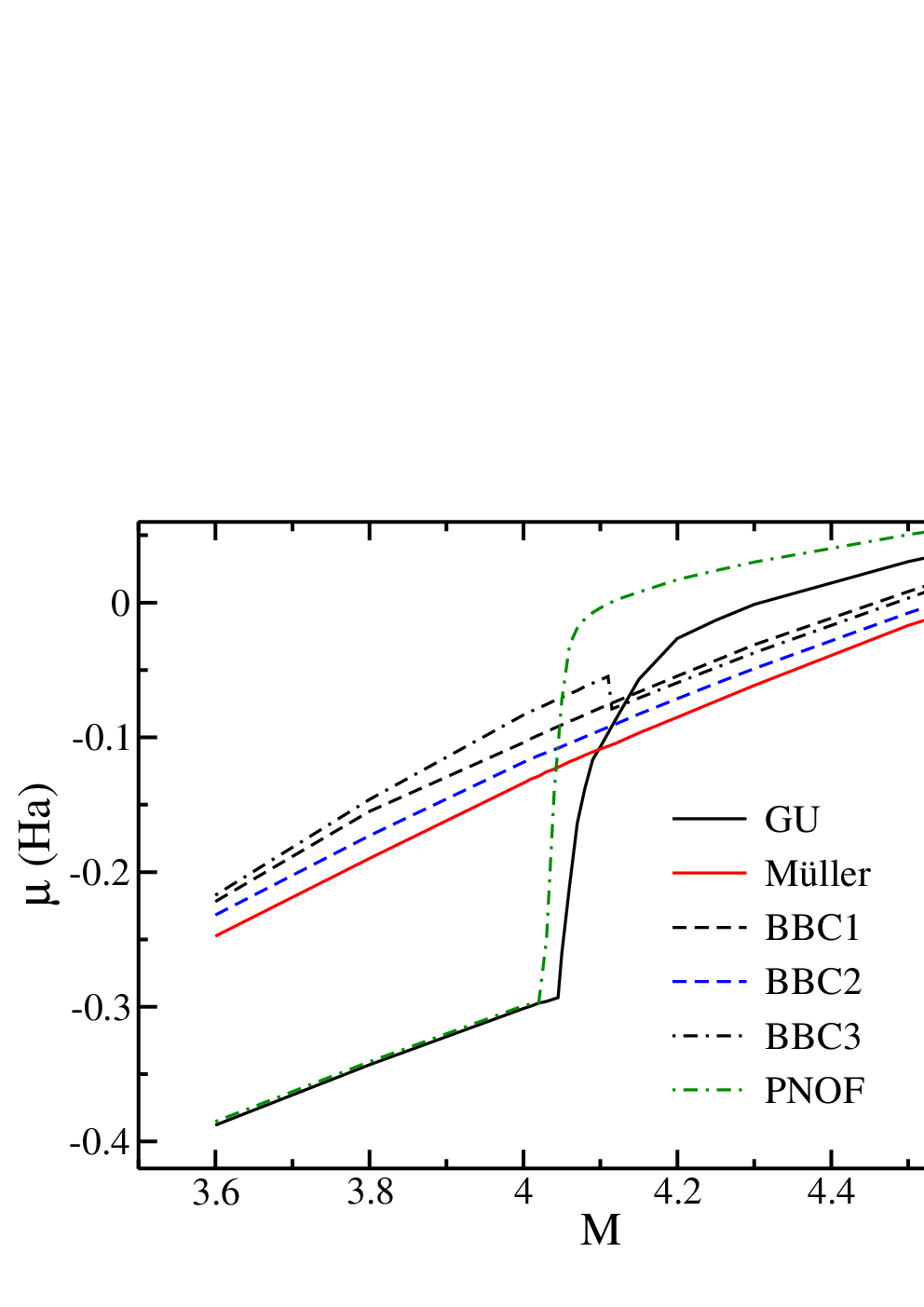
In all the calculations presented so far, we have used the functional of Goedecker and Umrigar, which involves the complete removal of the self-interaction terms. It is interesting to study the behavior of using different functionals, like for instance the recent BBC functionals of Gritsenko et al [7] and the PNOF of Piris[8, 9]. In the BBC1 and BBC2 functionals, the SI terms are present while in the BBC3, they are partially removed. However, the SI terms for the bonding and the anti-bonding orbitals remain. In the PNOF they are fully removed as in GU. In Fig. 6, we plot for LiH using the closed-shell treatment, for all these functionals. Surprisingly, only GU and PNOF show a pronounced step which compares well with the fundamental gap. The other functionals show either a completely smooth behavior or, in the case of BBC3, a small kink in the wrong direction. Therefore, we conclude that the complete removal of the SI terms is essential for obtaining the correct behavior of . The size of the step of for the PNOF is Ha and compares well with experiment (see Table 1). As a test, we also tried a modified version of BBC3 where we removed the SI terms completely. Consistent with the above conclusion, it also produces a step which is almost identical to PNOF. Additionally, this modified BBC3, like the GU functional, gives an accurate measure of the correlation energy at the equilibrium distance, but fails completely at the dissociation limit.
IV Conclusion
We have presented a formalism to calculate the fundamental gap within RDMFT for both open- as well as closed-shell systems. Our numerical results show that even for systems where the neutral system is closed-shell the results for the chemical potential are closer to the exact step function if an open-shell treatment is employed because adding charge of a specific spin to the system makes it open-shell. The application to several open-shell systems gives a very good agreement with experimental values in all cases. Also, the steps in the chemical potentials are such that they resemble the spin dependence of the ionization potential and the electron affinity of the real system. Our investigation of a possible basis set dependence reveals that it is necessary to include very diffuse states in the basis set in case the system does not bind extra charge. Whenever the system does bind extra charge the results are independent of the inclusion of the diffuse state in the basis set. To estimate the contribution of the occupation numbers and the natural orbitals to the fundamental gap we compared the results for the LiH molecule using a full variation and a variation of the occupation numbers only. We found that over 90% of the fundamental gap are due to the occupation numbers. This finding was confirmed for several other systems so far and we believe that it shows a general feature of RDMFT calculations. Finally, we investigated the behavior of several different functionals for the calculation of the fundamental gap. From our results we conclude that the exclusion of the self-interaction for all natural orbitals is essential to obtain reasonable results. Functionals without any removal of self-interaction simply yield a continuous chemical potential.
The present work is a contribution to the subject of calculating the fundamental gap of materials within RDMFT. The hope is that this theory gives results closer to experiment than DFT for this fundamental problem. It is our belief that the theoretical development presented in this work will have a significant impact in the application of RDMFT to periodic systems.
Acknowledgements.
We would like to thank A. Zacarias for valuable discussions on experimental and different theoretical results. This work was supported in part by the Deutsche Forschungsgemeinschaft within the program SPP 1145, and by EU’s Sixth Framework Program through the Nanoquanta Network of Excellence (NMP4-CT-2004-500198).References
- [1] P. Hohenberg and W. Kohn, Phys. Rev. 136, B 864 (1964).
- [2] W. Kohn and L. Sham, Phys. Rev. 140, A 1133 (1965).
- [3] T. Gilbert, Phys. Rev. B 12, 2111 (1975).
- [4] A. Müller, Phys. Lett. 105A, 446 (1984).
- [5] S. Goedecker and C. Umrigar, Phys. Rev. Lett. 81, 866 (1998).
- [6] M. Buijse and E. J. Baerends, Mol. Phys. 100, 401 (2002).
- [7] O. Gritsenko, K. Pernal, and E. J. Baerends, J. Chem. Phys. 122, 204102 (2005).
- [8] M. Piris, Int. J. Quant. Chem., 106, 1093 (2006)
- [9] P. Leiva, and M. Piris, J. Chem. Phys., 123, 214102 (2005)
- [10] N. N. Lathiotakis, N. Helbig, and E. K. U. Gross, Phys. Rev. B75, 195120 (2007).
- [11] J. P. Perdew and M. Levy, Phys. Rev. Lett. 51, 1884 (1983).
- [12] L. J. Sham and M. Schlüter, Phys. Rev. B 32, 3883 (1985).
- [13] M. Städele, J. A. Majewski, P. Vogl, and A. Görling, Phys. Rev. Lett. 79, 2089 (1997).
- [14] M. Städele et al., Phys. Rev. B 59, 10031 (1999).
- [15] S. Sharma, J. K. Dewhurst, and C. Ambrosch-Draxl, Phys. Rev. Lett. 95, 136402 (2005).
- [16] M. Grüning, A. Marini, and A. Rubio, J. Chem. Phys. 124, 154108 (2006).
- [17] J. Heyd, G. E. Scuseria, and M. Ernzerhof, J. Chem. Phys. 118, 8207 (2003).
- [18] J. Heyd and G. E. Scuseria, J. Chem. Phys. 120, 7274 (2004).
- [19] J. Heyd, J. E. Peralta, G. E. Scuseria, and R. L. Martin, J. Chem. Phys. 123, 174101 (2005).
- [20] J. P. Perdew, R. G. Parr, M. Levy, and J. L. Balduz, Jr., Phys. Rev. Lett. 49, 1691 (1982).
- [21] N. N. Lathiotakis, N. Helbig, and E. K. U. Gross, Phys. Rev. A 72, 030501 (2005).
- [22] P. Leiva, M Piris, Int. J. Quant. Chem. 107, 1 (2007).
- [23] L. J. Sham and M. Schlüter, Phys. Rev. Lett. 51, 1888 (1983).
- [24] W. Kohn, Phys. Rev. B 33, 4331 (1986).
- [25] A. Coleman, Rev. Mod. Phys. 35, 668 (1963).
- [26] N. Helbig, N. N. Lathiotakis, M. Albrecht, and E. K.U. Gross, Europhys. Lett., 77, 67003 (2007).
- [27] S. Sharma, N. Helbig, et al., in preparation.
- [28] M. W. Schmidt et al., J. Comp. Chem. 14, 1347 (1993).
- [29] J. A. Montgomery, Jr., J. W. Ochterski, and G. A. Petersson, J. Chem. Phys. 101, 5900 (1994).
- [30] A. A. Radzig and B. M. Smirnov, Reference Data on Atoms and Molecules (Springer Verlag, Berlin, 1985).
- [31] J. J. De Groote and M. Masili, J. Chem. Phys. 120, 2767 (2004).
- [32] H. R. Ihle and C. H. Wu, J. Chem. Phys. 63, 1605 (1975).
- [33] S. B. Sharp and G. I. Gellene, J. Chem. Phys. 113, 6122 (2000).