Gallager error correcting codes for binary asymmetric channels
Abstract
We derive critical noise levels for Gallager codes on asymmetric channels as a function of the input bias and the temperature. Using a statistical mechanics approach we study the space of codewords and the entropy in the various decoding regimes. We further discuss the relation of the convergence of the messsage passing algorithm with the endogeny property and complexity, characterizing solutions of recursive equations of distributions for cavity fields.
pacs
89.75.-k, 89.70.Kn, 75.10.Nr, 89.20.-a1 Introduction
Error-correcting codes play a central role in modern communication. These are used to communicate reliably in noisy media such as satellite and mobile communication. Currently, there is a wide range of error-correcting schemes, ranging from the classic Reed-Solomon codes [1], used today in mass storage media, to the more recent turbo codes [2] and low-density parity-check (LDPC) codes [3, 4] that have both shown near optimal performance.
Error-correcting codes exploit the idea of introducing redundancy into the message. The extra ‘redundant’ bits are constructed in a way known to both sender and receiver by correlating the message bits. If the channel noise is not too high the receiver can successfully decode and retrieve the exact original message. To minimize the transmission costs the amount of redundancy must be as small as possible. This inevitably makes the code more prone to errors; any good error correcting scheme must minimize both the required redundancy and the error probability. It is not at all a priory clear what are the limits in this trade-off. It was in 1948 that Claude Shannon blazed the trail [5] and proved that good error-correcting codes with arbitrarily small error probabilities do exist as long as the amount of redundancy is not smaller than a certain level, the so-called channel capacity.
However, Shannon’s groundbreaking proof was not suggestive as to how to construct practical useful codes that reach the Shannon limit. In 1962 Gallager proposed the family of the so-called low-density parity-check codes [3, 4]. Although conceptually simple, this coding scheme was largely forgotten due to the computational limitations of the time. Currently, however, with the advent of the computer era, they are recognized as one the best schemes available. The LDPC are easy to construct, have a low complexity and perform near the Shannon limit [6].
Gallager codes were re-discovered by MacKay and Neal [7] at around the same time when Sourlas [8] showed that statistical physics can be used to estimate the performance of error correcting codes. These two events brought in a surge of activity as well as an influx of research ideas from physics to information theory and vice versa. In particular, from a physics viewpoint, error-correcting codes have been so far studied quite extensively. For example, low-density parity-check ones on binary symmetric channels [9, 10, 11, 12, 13], on real-valued channels [14, 15], on irregular graphs [16] while more recently the error exponent was calculated in [17, 18]. Turbo codes have been studied in [19, 20]. For a more complete review on the subject see [21, 22]. Clearly, the bibliography of statistical physics of codes is largely biased towards the low-density parity-check ones: this is because the recently developed finite-connectivity techniques offer an ideal toolbox for the theoretical study of this field. Currently, the more recent developments in the physics of finitely connected systems allow one to extend previous results with algorithms that perform better [23, 24, 25]. Altough these algorithms reach the computational limits of today, maybe one day they will also become useful.
Qualitatively speaking the emerging picture for Gallager codes is that for sufficiently small noise levels, decoding with a message-passing algorithm with a linear computational complexity in the block size is possible and the error-free state is the only stable state. For higher noise levels, one finds a transition to a regime where suboptimal states are created (marking the so-called spinodal or dynamical transition) and where the message passing algorithms fail to find the most probable solution. For higher noise levels, a second transition occurs (thermodynamic transition) where the error-free solution ceases to be dominant. This marks the upper theoretical bound for error-free communication. This means that block-wise maximum likelihood decoding, which is shown to be NP-complete [26], fails.
In this paper we study Gallager codes on the family of binary asymmetric channels (BAC). The two extreme cases of this family include the binary symmetric channel (which has been the key actor in nearly all previous research) and the (fully asymmetric) Z-channel. The latter is used in communications through optical fibers. Within replica symmetry we calculate the location of the static and dynamic transitions. We also present phase diagrams describing where the frozen phase and clustered phases appear. As a reference point to test our theory we have used known results from information theory [27] and shown that it reproduces them with very good agreement.
Our paper is organized as follows: In the following section we provide the model definitions for Gallager codes and the decoding process. In section 3 we set up the decoding problem in statistical mechanical terms. In section 4 we derive the thermodynamic quantities for a simple limiting case (dense codes) while in section 5 we compute the free energy of the binary asymmetric channel. In section 6 we discuss the failure of belief propagation (BP) while in section 7 we present results from a one-step replica symmetry-breaking scheme. We end this paper with a discussion in section 8.
2 Model definitions
2.1 Gallager codes
The aim is to send a message reliably through a noisy medium. Hereby four processes are of importance: the generation of the message by the source, the encoding process, the noise and the decoding process.
We consider a source which produces messages with probability
| (1) |
with the bias of the input signal.

The message is sent from one point to another through a noisy channel. To communicate the message in an error-free way redundant bits are added to the message before it is sent through the channel (encoding process). The encoding process is defined by the map , with . The elements of the image of are called the codewords. Shannon, in his original paper [5], showed that for a family of codes, having a completely random set of codewords, it is possible for to decode errorlessly with probability one as long as the code rate , with the binary entropy, is smaller or equal to the maximal admissible amount of information we can send through the channel. This is given by the so-called channel capacity (see A for a computation of the channel capacity for the BAC). However, as Shannon’s random encoding turns out to be inefficient for practical error correction a new encoding/decoding strategy was sought. Gallager, among others, proposed a scheme for introducing more structure in the set of codewords [3, 4]. In particular, he suggested the linear space of codewords:
| (2) |
with
| (3) |
is the parity check matrix which is a sparse matrix with elements . The symbol denotes concatenation of two matrices. The matrix is of dimension and is an invertible matrix of dimension . The elements of and lie in . In regular Gallager codes the parity check matrix is constructed such that there are non-zero elements per row and non-zero elements per column. In irregular codes the number of ones per row and per columns are drawn from a distribution. Counting the number of ones in this matrix provides for regular codes the relation which expresses the code rate in terms of the code parameters. The equations implied by (2) are the parity-check equations. Using Gaussian elimination one can bring to a systematic form described by with such that and where is the identity matrix. The matrices and span the same space and are thus equivalent parity check matrices. We can now define the generator matrix such that due to the mod-2 arithmetic one obtains . With these definitions encoding is realized through . This implies that for .
Channel noise can be seen as a bit-flipping operation. The effect of noise can be presented as a transformation , where represents the channel true noise vector. The channel can be represented by the probability of a true noise vector given the message. For the BAC, equals (figure 1),
| (4) |
with
| (5) |
The parameters give the bit-flip probabilities of the channel. In (4) we assumed that the channel is memoryless. For convenience we define the variable such that the binary symmetric channel corresponds to while for one obtains the fully asymmetric Z-channel, which is of interest for optical communication (with the two states representing the presence or absence of light in the channel).
The receiver at the other end of the channel uses a prescribed set of operations to extract the original message from the received word (decoding). After obtaining the bit stream the receiver is required to solve, using the aforementioned properties of the generator matrix, the equations . Among the solutions of these equations an estimate for the true noise is obtained. Once this is found an estimate for the original message immediately follows. The estimates of the single bits are obtained by calculating the single bit marginals
| (6) |
The notation denotes the set of components of excluding the -th. The choice of determines the decoding process while are the variables of this decoding process. At first sight it seems impossible to calculate these quantities as we need operations. However, LDPC codes owe their success in the existence of a belief-propagation algorithm [28] (see also [9, 29]), whose computational complexity scales linearly in the system size , able to calculate the above marginals. This is achieved by interpreting the parity check equations of (2) as a bipartite graph (the so-called Tanner graph) in which variable nodes, associated to each , are connected to check nodes associated to each of the constraints of (2).
The performance of the code can be determined through a loss function [30]. If we take as loss function , which is the overlap between the true noise vector and the variables of the decoding process, the optimal estimator can be shown to be given by [31]. Thus we measure the performance through the order parameter defined as
| (7) |
The brackets denote the average over (6) and the bar denotes the average over and .
2.2 Decoding processes
Without loss of generality we can represent the conditional probability through
| (8) |
distinguishing between different states for each received bit. The subindex corresponds with the value of the received bit . The normalization constant is independent of the decoding variables and will be left out. This will be important for the calculation of the entropy. The parameters and , also called the Nishimori parameters, determine the decoding scheme in the case of symbol-wise maximum a-posteriori probability (symbol-wise MAP). In symbol-wise MAP we want to choose the probability distribution such that is maximal. Following [30] we can find these parameters by identifying (8) with the true posterior probability distribution determined by the characteristics of the source and the channel noise. Using Bayes’ rule we obtain
| (9) |
and
| (10) |
One can easily write down the probabilities and from the channel description of figure 1. For instance . For the a priory probability of codewords we have
| (11) |
since the first bits of the codeword are copies of the original message and all codewords must satisfy (2). From we then find that the Nishimori parameters become
| (12) | |||||
| (13) |
In general we will consider decoding processes where . When we get block-wise MAP decoding. We remark that for unbiased channels symbol-wise and block-wise MAP decoders perform the same as symbol-wise and block-wise maximum likelihood decoders.
3 Statistical mechanics for Gallager codes
3.1 The partition function
To begin the statistical mechanical analysis of the decoding process we define the equilibrium Boltzmann measure of candidate noise vectors given the parity check matrix, the true noise vector and the received bit stream:
| (14) |
where represents the partition function of our system:
| (15) |
To find the behavior of in (7), we calculate the typical value of the free energy for . Assuming self-averaging we can find by calculating the code- and noise-averaged free energy , given by
| (16) |
The hardcore restriction, which imposes that candidate noise vectors must satisfy the parity checks, can be written as
| (17) |
with and
The probability distribution of the tensor follows from the statistics of , namely
| (21) |
is the normalization constant, i.e. . We have used the notation to denote the ordered set . The joint probability in (16) does not factorize due to the asymmetry of the channel. It can be evaluated through
| (22) |
After making the gauge transformation , we have the following partition function
| (23) |
modulo irrelevant multiplicative constants. The quenched fields are drawn from the distribution
| (24) |
with
| (25) |
and .
3.2 Gauge transformation
The gauge theory of disordered systems, pioneered by Nishimori [32], uses symmetry relations to derive a number of exact results. Of particular interest is the Nishimori line on which one can compute exactly the internal energy and one can show that there are no replica symmetry breaking effects. For error correcting codes, using symbol-wise MAP decoding with turns out to be equivalent to computing decoding observables on the Nishimori line.
For an unbiased BSC we have . This model falls then in the category of channels characterized in [10]. Since the above distribution (25) fullfils the conditions we can write the free energy in a more symmetric form as in [10]. For any observable we can write
| (26) |
with
| (27) |
Making the transformations and also , with , we arrive at the more symmetric form
with . At we can, using the techniques in [31], exploit this symmetry to prove that the thermodynamic state is replica symmetric. The energy at equals
| (29) | |||||
The distribution is defined as
| (30) |
The average is over . One can also prove that which is equivalent to the statement that corresponds with MPM decoding [33].
4 A simple solvable detour: The random codeword model


Before we embark on the evaluation of the finitely connected case, we consider the simple limiting case of . This limit, implying an infinite number of parity checks, is of course of small practical importance but nevertheless very educational as it already contains a wealth of information about the code’s performance. It will also give us a first flavour about the effects of asymmetry in Gallager codes. In this limit it can be shown that the codewords , for an unbiased source, are sampled with a flat probability, thus this model is coined the ‘random codeword model’ (RCM). These codewords determine the paramagnetic behavior of the system. Besides these, the model also contains the ferromagnetic state . We choose . We could say that this choice identifies , which corresponds with the analysis done before. Below we follow the derivation as given in [10]. The energies of the codewords, after the gauge transformation , are given by
| (31) |
with and . The entropy of these states, for a given and , is equal to
| (32) |
with . The limit of maximum likelihood decoding is given by the noise levels where , with the magnetizations of the ferromagnetic state:
| (33) |
This zero entropy condition corresponds to , with the mutual information for an asymmetric channel, see equation (104). We thus find the Shannon limit back, see also figure 2. In finite temperature decoding we restrict the energies and by introducing the Lagrange parameters and . The free energy is defined through the Legendre transformation
| (34) |
We find that the entropy as a function of and , becomes zero when , with
| (35) | |||||||
The entropy can become negative as a result of having a partition sum dominated by atypical states. The number of these states becomes zero when . This corresponds with an entropy crisis as found in the random energy model [34], [35]. To avoid this we will introduce the spin glass phase corresponding with the ground states of the system. The spin glass state has a free energy given by
| (36) |
with . The paramagnetic free energy is given by
Comparing the free energies of the ferromagnetic, paramagnetic and spin glass state we find for the phase diagram presented in figure 3. We remark that increasing the degree of asymmetry in the channel noise leads to a bigger ferromagnetic region. The ferromagnetic-spin glass phase transition is given by . The triple point lies at .

5 Free energy and saddle point equations
In the more general case, the evaluation of the free energy (16) and of the various thermodynamic properties can be done either with the replica [36, 37, 38] or the cavity method [39, 40], both of which have been shown to lead to identical results. Although the two methods differ in their philosophy, they can be seen as two complementary sides of the same coin, and together they can offer a more complete understanding of the physics of the system under study. We follow here the replica methodology and postpone our discussion on the cavity method for B. The free energy is of the form
| (38) |
with
| (39) |
with the partition function given by (23). This expression, describing an average over parity check matrices and input codewords, can be dealt with using the replica method [39]. We replicate the -variables times to and the variables times to . The free energy per bit (16) is then given by an extremization problem:
| (40) |
The function equals
| (41) |
with
| (42) |
The order parameters and are solutions of the self-consistent equations
| (43) | |||
| (44) |
Inserting (43) into (44) produces a single self-consistent equation in terms of .
5.1 Replica Symmetry

For the joint distribution of the replicated spin variables we now write
| (45) |
In order to take the limit , one has to make an assumption for the form of the distribution . The simplest such ansatz corresponds to replica symmetry, i.e. assuming that the -replica indices with respect to the noise variables are inter-changable. More concretely we write
| (46) |
for some with . Using this ansatz we can convert the self-consistent equation of into one for the density and one for , namely
| (47) | |||
We defined the messages
| (48) |
To take the limit we make the following assumptions on the -dependencies
| (49) | |||||
with and . The distribution fullfills the self-consistent equation
| (51) |
with . The distribution turns out to be also a solution of the equation (51). The distributions are given through the equations
| (52) |
with and and
| (53) |
Equations (51) and (52) are the main equations from which the various thermodynamic quantities in this section will be derived. We remark that the distribution gives the distribution of cavity fields given the value of on the corresponding link and the value of and on the corresponding site. Finally we have to average over and . Substitution of the ansätze (45), (46), (49) and () in the expression (41) of the free energy leads to, after taking the limits and
| (54) |
with
| (55) | |||
| (56) |
and where we used the abbreviations
| (57) | |||||
| (58) | |||||
| (59) |
In the unbiased case , we have the stable solution and with
| (60) |
and
| (61) |
with
| (62) | |||
| (63) |

We see that for unbiased sources the formulas (52) and (54) are much simplified to (60) and (61). Generalization of these formulas to irregular graphs is straightforward. We note that and correspond, in the framework of the cavity method [41], to the free energy shifts due to link- and site-addition respectively. Equation (60) is also known as the ‘density evolution’ equation (while the equivalent (121) of B which refers to a single graph instance is termed as the ‘belief propagation’ equation).
We see that the state is always a solution to (52) and gives . If the initial state lies in the basin of attraction of this solution, errorless decoding is possible. We will term this the ferromagnetic solution. The ferromagnetic state has a free energy equal to
| (64) | |||||
From equations (61), (64) we see that for , the free energy becomes . To avoid these infinities we will solve the problem for and look at quantities that are finite for .
| 5 | 6 | 0.13739(5) | 0.26436(3) | 0.35546(2) | 0.70400(5) | 0.28709(2) | 0.54800(1) |
|---|---|---|---|---|---|---|---|
| 3 | 4 | 0.16703(1) | 0.20959(1) | 0.45580(2) | 0.57591(4) | 0.35426(1) | 0.44167(1) |
| 4 | 6 | 0.11692(1) | 0.17245(1) | 0.30802(2) | 0.47132(5) | 0.24615(1) | 0.36373(2) |
| 3 | 6 | 0.08406(1) | 0.09972(1) | 0.23146(2) | 0.27880(1) | 0.17977(2) | 0.21329(2) |
| 4 | 8 | 0.07681(1) | 0.10717(1) | 0.20056(2) | 0.2905(1) | 0.16137(2) | 0.22635(2) |

We solve the coupled set of equations (51) and (52) using a methodology similar qto ‘population dynamics’ [40]. We first derive the stationary distribution for the density (51) describing a population of -fields . We remark that since we need not to update separately a population of -fields. For every -field we associate a -population of -fields, namely . A stationary solution for the population of populations of -fields is found through the following algorithm:
- 1.
We select fields from the -population: with and the set of chosen indices .
- 2.
We calculate a new -field according to its update rule:
- 3.
We use the populations of -fields indexed by to calculate a new population of -fields with the update rule
- 4.
We select at random an index and replace the -th member of the -population by and the -th member of the -population by .
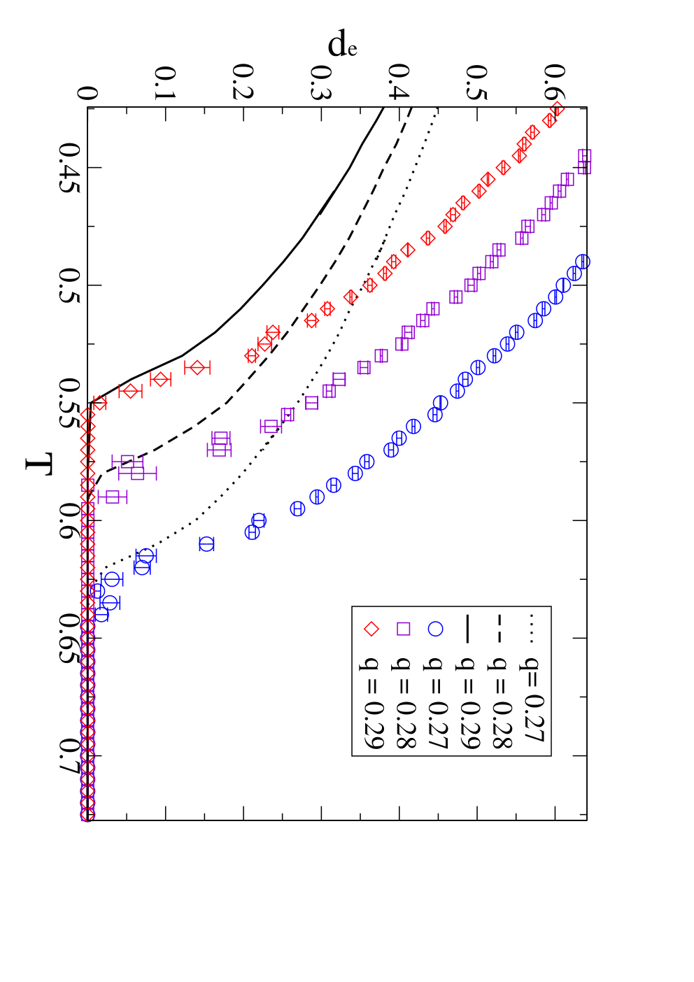
We start with the initial distribution . This corresponds to a state with no a priory knowledge on the message . At low temperature this distribution converges to the ferromagnetic state. Increasing the noise at a constant temperature we find that at some critical noise level a second solution appears (suboptimal solution) with . We remark that below the -threshold, the ferromagnetic state is the only stable state for all initial conditions. From an algorithmic point of view is the threshold to successful decoding with the belief propagation algorithm. The thermodynamic transition is determined by the point where the free energy of the suboptimal solution becomes lower then the free energy of the ferromagnetic solution. At this determines the limit for maximum likelihood decoding. In figure 4 we see that when we increase and keep the rate constant, the limit for maximum likelihood decoding increases but the limit for belief propagation decoding decreases. Indeed, we found that in the RCM the paramagnetic state is always stable. We find that, in contrary to the cases of symmetric channels, the bias in the input signal influences the decoding process. However, comparing the critical noise levels , above which errorless decoding is impossible for all type of encoding processes, between an optimal biased source and an unbiased source, see figure 15, we see that bias has few influence. In figure 5 we show, for a Z-channel, how these thresholds get influenced by the bias. For a BSC the minimum lies at , whereas for a Z-channel the minimum channel noise lies at a point . We also compared our results obtained through population dynamics with a specific application of the belief propagation algorithm on a specific graph instance. The results of both methods match very well. In table 1 we present the spinodal and thermodynamic critical values for different regular codes and for various degrees of symmetry. These results are consistent with values found in [22, 11] and in good agreement with those of [27]. In figure 6 we present the spinodal transition lines for different values of the inverse temperature and the parameter . We find re-entrance effects below the Nishimori line. We find these re-entrance effects also in the thermodynamic lines. In figure 7 we plot the entropy , with determined through equation (61), as a function of the channel parameters. We see that it becomes negative at the spinodal noise level . The entropy at the Nishimori temperature has a special meaning as it is the average entropy of the transmitted message once the received message is known. This is therefore the theoretical upper limit irrespectively of the decoding dynamics. The energy at , see equation (29), equals the ferromagnetic energy (64). From this it follows that the entropy at becomes greater than zero at the critical noise level . Performing a large expansion of (60) and (61), as done for the BSC in [10], we get for the critical noise levels, taking constant,
| (65) |
with . The function is given by
| (66) |
From (65) we find for a (3,6)-code when , and , . For a (3,4)-code we find when , and when , .
5.2 The entropy crisis
From figure 7 we have learned that the entropy can indeed become negative for the asymmetric channel. We also found re-entrance effects in the thermodynamic transition lines. This indicates that something is missing in our solution. In the SK-model [39], the negative entropy in the ground state is an indication that the replica symmetric formalism is incorrect. In general -spin models, see [42], we have at a temperature a transition from a paramagnetic phase to a one step replica symmetry breaking phase and at a temperature an entropy crisis corresponding with the vanishing of the configurational entropy. Here, though, because of the infinitely strong interactions, the first phase transition will not appear [43]. We will have an entropy crisis just like it occurs in the RCM. Because we are interested in the typical behavior of the system we should define the typical free energy , as
| (67) |
where is the inverse temperature at which the system freezes in the lowest energy paramagnetic configuration, i.e. .


Because of the hard constraints, we have indeed that following frozen ansatz, see [10],
| (68) |
with , fullfills the selfconsitent equations (44) . Using this ansatz in the self-consistent equations (44) and the free energy expression (41), we find back the replica symmetric equations (52) and (54) with . The extremization condition corresponds to the zero entropy condition, which for can only be fullfilled when . When we have , because there the free energy is indeed maximal. This corresponds with the frozen scenario of (67). We will call the phase where the entropy is zero and the spin glass phase and the phase where and the paramagnetic phase. In the spin glass phase the thermodynamic average is dominated by a subexponential amount (in the system size) of codewords whereas in the paramagnetic phase the average is dominated by an exponential amount of codewords. In figure 8 we plot the full thermodynamic phase diagram of the system in the space of for a regular code with an unbiased source and three different levels of symmetry in the channel noise. The re-entrance effects have disappeared because of the frozen ansatz.
6 Non-convergence regions of belief propagation and endogeny

Although the freezing scenario presented above seems to explain the thermodynamical phase diagram completely, the dynamics of the system can be disturbed by a clustering of the phase space. To investigate this more closely we will consider a system composed of two copies of the original dynamic variables. These are embedded on the same graph and interact with the same quenched fields. In this setting, convergence of the recursive decoding equations can be quantified through the resulting statistics of the joint system.
We remark that the convergence of the belief propagation equations can be seen as one example of a general class of problems in which one is interested in the stationary density that solves a distributional fixed-point problem. This problem and its applications to various fields has been studied in a rigorous way by Aldous and Bandyopadhyay [44] from the viewpoint of theoretical statistics. This link between the two fields has been observed in [45].
In the case of a two-replica system we define a partition function of a form similar to (23):
| (69) |
with . Analagously as in section 5 we find for the unbiased case, the following order parameter equations
| (70) | |||
| (71) |
We introduce the replica symmetric ansatz
| (72) |
We remark that a field coupling the and variables is not needed because in (71) the quenched field does not couple and variables. Substitution of this ansatz in the above self-consistent equations leads to
| (73) |
Now we check whether the distribution , with the solution to (60), converges to (note that all computations are done within RS). We introduce the quantity
| (74) |
We remark that corresponds in the two replica formalism to and hence corresponds with some sort of spin glass behavior in the same sense as in the SK model. This two replica formalism is, in certain models, proven to be equivalent with the endogenous property, see [44]. The failure of the endogenous property has serious consequences on the convergence of the BP equations. We define
| (75) |
with the log-likelihood ratio on site on the time step of the BP algorithm (121). As long as , the BP equations converge. In figure 9 we compare the parameter of both formalism and we find that indeed when the BP equations stop converging. We call the line marking the transition from to the endogeny line. In figures 10 and 11 we present this line respectively for a Z-channel and a BSC, together with the different thermodynamic and spinodal lines. In table 2 we give a summary of the various regions of the phase diagrams in figures 10 and 11. Performing a high connectivity expansion, like is done in [10] we find that the endogeny parameter of the paramagnetic solution is zero.


7 1RSB ansatz
From the results of the previous section we know that replica symmetry fails below a certain temperature. The non-convergence of the belief propagation equations below a certain temperature reveals that the amount of solutions of the belief propagation equations (121) scales exponentially with the system size. This can be solved using replica symmetry breaking, which correspond to a more advanced algorithm. In optimization problems, using insights of 1RSB-effects, practical algorithms have been found (see [46]). To count the number of the solutions of (121), we introduce a Lagrange parameter conjugate to the free energy of these solutions. We have a generalized free energy corresponding with
| (76) |
with a sum over pure states. By pure states we are referring to independent ergodic components in our system. If we call with the free energy of state we see that
| (77) |
with
| (78) |
These quantities can be calculated through the following ansatz (see [47]),
| (79) |
for some functional with . Replicas here are only interchangeable within the group to which they belong. Spin variables carry two indices denoting the group and replica within the group. This one-step replica symmetry breaking has been considered for the binary symmetric channel in [23].
Substituting this ansatz into the self-consistent equations (44) results in, using ,
| (80) |
where denotes a functional delta distribution in the sense that . We also introduced the distribution , equal to:
| (81) |
In (81) is given by
| (82) |
which in terms of the cavity terminology equals the free energy shift due to iteration. When we focus from now on on the unbiased case we get a somewhat simpler expression:
| (83) |
In principle this equation can be solved with the iterative scheme of population dynamics [40]. Substitution of (79) and (80) in (41) produces an expression for the generalized free energy
| (84) |
with the averages
| (85) | |||
| (86) |
The generalized free energy shifts and are given by:
| (87) | |||||
| (88) |
The free energy follows from :
| (89) |
with
| (90) | |||||
| (91) |
Combining (84) and (89) produces finally the complexity:
| (92) |
as a function of the free energy. An alternative way to derive the above is based on the cavity method (see B) which shows that the complexity corresponds to the entropy of the number of solutions to the cavity equations with free energy density .


7.1 A special case: the frozen-ansatz
The general scheme described by (80) allows one to retrieve the solutions of the frozen ansatz (68). This can be done by considering solutions of the form
| (93) |
This solution can be interpreted as having on each site a probability to have a state with . The distribution corresponds to site averages. In the case where is even, it is clear that (93) is a solution of the 1RSB self-consistent equations (80). For odd the reweighting factor in (80) makes sure that the zero fields do not appear. Hence (93) is also a solution of (80) when is odd. Substitution of (93) in (80) gives the following self-consistent equation for the distribution
TheseequationsturnouttobeequivalenttotheRSequations(60),wefoundbefore.Thiscanbeseenbysubstitutinga =exp(μx)/(2cosh(βx))μ= βf_RS(Φ_1RSB)s_RS = 0 (Σ_1RSB = 0)β¡β_gm=1β¿β_gm=β_g/βs_α = 0(p_c,q_c)(p_c,q_c)T=1
7.2 The more general case: the complete 1RSB

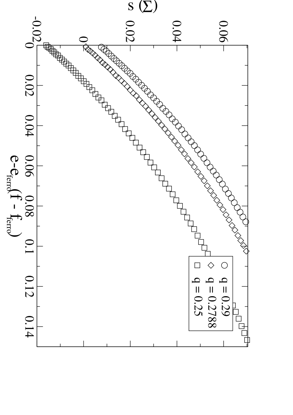
Finally we consider the solution of the 1RSB equations (83) and (84). Numerically the 1RSB approach is prone to many errors coming from the small sizes of the distributions (we used 1000 distributions of each 1000 fields). We also emphasize that the 1RSB replica and cavity method may contain many non controllable approximations. This is especially true for the complexity, see [48] and [49]. With this in mind we try to interpret the result presented in figure 14, which has been calculated for parameter values corresponding to the marked points of the phase diagram in figure 11. At the point marked with a cross we find a zero complexity for all values of . At the dotted marker we find a positive complexity for some values of . From the thermodynamical relation between and , we know that must decrease as a function of . Eliminating the branches where the complexity increases as a function of we find the results in figure 14. We find a regime with a positive complexity and a negative entropy. This means that there is an exponential number of solutions to the belief propagation equations and thus the belief propagation algorithm does no longer converge. We also remark that the fact that these solutions have a negative entropy is consistent with the freezing picture we found in section 7.1. It would be interesting to look for the change of the dynamic thresholds between the replica symmetric and 1RSB algorithms. In order to exclude finite size effects, we would need larger system sizes to determine accurately these thresholds.
8 Discussion
In this paper we study the decoding properties of LDPC-codes on a binary asymmetric channel, using tools from statistical mechanics on finitely connected systems. As a result of the channel asymmetry the microscopic Boltzmann distribution for the channel noise inherits an explicit dependence on the received message. This results in a set of recursive equations for two types of cavity fields. We determine the decoding thresholds for message passing algorithms as a function of the important parameters, e.g. the asymmetry, the bias and the temperature. Calculating the entropy we find the upper bound to any decoding scheme.
For dense codes we retrieve the random codeword model. The thermodynamic averages are characterized by the existence of a ferromagnetic, spin glass and paramagnetic phase. The ferromagnetic region increases with increasing asymmetry in the channel noise. Because the paramagnetic solution is always stable, the message passing algorithms fail to decode correctly the received message at all noise levels.
For low-density codes the emerging picture in the temperature-noise phase diagram is that for high temperatures we find two solutions for the cavity distributions. For these temperatures and low noise levels there is a ferromagnetic phase indicating succesful decoding. Increasing the noise level to a certain threshold the appearance of a paramagnetic solution distorts the decoding process. As the temperature is lowered this paramagnetic solution freezes into a zero-entropy solution, representing a subexponential number of codewords. Lowering the temperature even further the decoding dynamics of the system is distorted by an exponential number of metastable states. We discuss this failure in terms of the endogeny property of the recursive equations for the cavity fields.
Appendix A The capacity of the binary asymmetric channel
Shannon’s famous channel coding theorem states that error free communication can be possible as long as the rate is kept below a certain critical value , the channel capacity. We use the abbreviation for the binary entropy, . We here calculate the channel capacity for the binary asymmetric channel. It is defined as
| (102) |
where is the set of possible inputs to the channel and the set of possible outputs. The average mutual information
| (103) |
written in terms of the marginal- and conditional entropy represents the amount of information carried by the channel for a given noise probability. Thus provides the maximum admissible amount of information carried by the channel. In the case of a binary alphabet with and with we find that for the binary asymmetric channel, see figure 1, the mutual information is given by
| (104) |
The maximum of with respect to is attained at
| (105) |
with , provided that . Indeed, we see in figure (15) that at constant rate the channel noise gets a maximum at some . If on the other hand we keep the code fixed, and we take into consideration that the parity check bits are unbiased, we get a minimum value at .

Appendix B Cavity method
We can derive mean field equations for a specific graph instance using the cavity method [41]. The cavity method gives us a link between the different mean field solutions we find using the replica method and different decoding algorithms. First, we derive the cavity equations for a typical solution with a weight given by (11). We define the cavity graph as a graph having spins connected to hyperedges and cavity spins connected to hyperedges. On this graph we consider the graph operations defined in [41]: site addition, link addition and site iteration. We will try to count how the number of solutions to the equations,
| (106) |
corresponding with an energy density , change when performing the aforementioned graph operations. If is the set of solutions of (106), we define
| (107) |
is the entropy and are the quenched fields. Suppose we are only interested in small fluctuations around some reference energy . The probability that a configuration has an energy is then given by
| (108) |
with . We define through a Legendre transform the free energy F
| (109) |
We use the notation for the entropy density on the graph . Site addition is the graph operation which adds a site to connecting it with hyperedges to cavity spins. Under site addition , we assume that fullfills
| (110) |
where is the distribution of energy changes under site addition. From (110) we have
| (111) |
The free energy change under site addition, , is thus equal to
| (112) |
Link addition is the graph operation which adds a hyperedge between K cavity spins. Under this operation we find for
The free energy change under link addition becomes
| (114) |
When we start from a graph , we can perform K site additions or link additions to get a graph without cavity spins. In the limit we get
| (115) |
The distributions and are given by
| (116) |
with the external field at the new site. is the distribution of the spins on site when we go to a state with energy E. We assumed that the probabilities of the cavity spins are uncorrelated. It is possible to find a recursion relation for through
| (117) |
The joint probability of the spin at the new site, and the energy after iteration is
| (118) |
with
| (119) |
We see that the dependency disappears. We can parametrize the spin distributions as
| (120) |
to get the cavity or belief propagation equations
| (121) |
From (121) we can retrieve the equations (52), using
| (122) |
and the assumption that we have large loops in the graph. We find for the free energy changes and
| (123) | |||
| (124) |
Sometimes the cavity equations (121) do not converge because there are many solutions to these equations and each part of the graph converges to different kind of solutions. The reason is that the cavity spins are not uncorrelated. In that case we assume that there are solutions to the cavity equations with free energy f, i.e.
| (125) |
We then find through a complete analogue calculation as above the 1RSB equations on a specific graph instance. In that case .
References
References
- [1] I. S. Reed and G. Solomon, “Polynomial codes over certain finite fields,” SIAM Journal of Applied Mathematics, vol. 8, p. 300, 1960.
- [2] C. Berrou, A. Glavieux, and R. Thitimajshima, “Near shannon limit error-correcting coding and decoding: Turbo codes,” Proc. IEEE Int. Conf. Commun., p. 1064, 1993.
- [3] R. Gallager, “Low density parity check codes,” IRE Trans. Info. Theory, vol. 8, p. 21, 1962.
- [4] R. Gallager, Low density parity check codes, vol. 21 of Research Monograph Series. Cambridge MA: MIT Press, 1963.
- [5] C. E. Shannon, “A mathematical theory of communication,” Bell System Tech. J., vol. 27, pp. 379, 623, 1948.
- [6] T. Richardson and R. Urbanke, “The renaissance of gallager’s low-density parity-check codes,” IEEE Commun. Mag., vol. 41, p. 126, 2003.
- [7] D. J. C. MacKay and R. M. Neal, “Near shannon limit performance of low density parity check codes,” IEE Electronic Letters, vol. 32, p. 1645, 1996.
- [8] N. Sourlas, “Spin-glass models as error-correcting codes,” Nature, vol. 339, p. 693, 1989.
- [9] R. Vicente, D. Saad, and Y. Kabashima, “Finite-connectivity systems as error-correcting codes,” Phys. Rev. E, vol. 60, p. 5352, 1999.
- [10] A. Montanari, “The glassy phase of gallager codes,” Eur. Phys. J. B, vol. 23, p. 121, 2001.
- [11] S. Franz, M. Leone, A. Montanari, and F. Ricci-Tersenghi, “The dynamic phase transition for decoding algorithms,” Phys. Rev. E, vol. 66, p. 046120, 2002.
- [12] Y. Kabashima and D. Saad, “Statistical mechanics of error-correcting codes,” Europhys. Lett., vol. 45, p. 97, 1999.
- [13] T. Murayama, Y. Kabashima, D. Saad, and R. Vicente, “Statistical physics of regular low-density parity-check error-correcting codes,” Phys. Rev. E, vol. 62, p. 1577, 2000.
- [14] N. S. Skantzos, J. van Mourik, and D. Saad, “Magnetisation enumerator for real valued symmetric channels in gallager error-correcting codes,” Phys. Rev. E, vol. 67, p. 037101, 2003.
- [15] T. Tanaka and D. Saad, “Typical performance of regular low-density parity-check codes over general symmetric channels,” J. Phys. A: Math. Gen., vol. 36, p. 11143, 2003.
- [16] R. Vicente, D. Saad, and Y. Kabashima, “Statistical physics of irregular low-density parity-check nodes,” J. Phys. A: Math. Gen., vol. 33, p. 6527, 2000.
- [17] N. S. Skantzos, J. van Mourik, D. Saad, and Y. Kabashima, “Average and reliability error exponents in low-density parity-check codes,” J. Phys. A: Math. Gen., vol. 36, p. 11131, 2003.
- [18] T. Mora and O. Rivoire, “Statistical mechanics of error exponents for error-correcting codes,” Phys. Rev. E, vol. 74, p. 056110, 2006.
- [19] A. Montanari and N. Sourlas, “The statistical mechanics of turbo codes,” Eur. Phys. J. B, vol. 18, p. 107, 2000.
- [20] A. Montanari, “Turbo codes: the phase transition,” Eur. Phys. J. B, vol. 18, p. 121, 2000.
- [21] Y. Kabashima and D. Saad, “Statistical mechanics of low-density parity-checks codes,” J. Phys. A: Math. Gen., vol. 37, p. R1, 2004.
- [22] A. Montanari and R. Urbanke, “Modern coding theory: The statistical mechanics and computer science point of view.” Lectures at Les Houches Summer School on ‘Complex Systems’, 2006.
- [23] G. Migliorini and D. Saad, “Finite-connectivity spin-glass phase diagrams and low-density parity check codes,” Phys. Rev. E, vol. 73, p. 026122, 2006.
- [24] J. P. L. Hatchett and Y. Kabashima, “Survey propagation for the cascading sourlas code,” J. Phys. A: Math. Gen., vol. 39, p. 10659, 2006.
- [25] B. Wemmenhove and B. Kappen, “Survey propagation at finite temperature: application to a sourlas code as a toy model,” J. Phys. A: Math. Gen., vol. 39, p. 1265, 2006.
- [26] E. R. Berlekamp, R. J. McEliece, and H. C. A. van Tilborg, “On the inherent intractability of certain coding problems,” IEEE Trans. Inform. Theory, vol. 24, p. 384, 1978.
- [27] C. Wang, S. R. Kulkarni, and H. V. Poor, “Density evolution for asymmetric memoryless channels,” IEEE Trans. on Inf. Theory, vol. 51, p. 4216, 2005.
- [28] J. Pearl, Probabilistic Reasoning in Intelligent Systems: Networks of Plausible Inference. San Francisco, CA: Morgan Kaufmann, revised second printing ed., 1988.
- [29] J. S. Yedidia, W. T. Freeman, and Y. Weiss, Exploring Artificial Intelligence in the New Millennium, ch. 8, p. 236. Science & Technology Books, 2006.
- [30] Y. Iba, “The nishimori line and bayesian statistics,” J. Phys. A: Math. Gen., vol. 32, p. 3875, 1999.
- [31] H. Nishimori, Statistical physics of spin glasses and information processing. Oxford Science publication, 2001.
- [32] H. Nishimori, “Internal energy, specific heat and correlation function of the bond-random ising model,” J. Phys. Soc. Japan, vol. 66, p. 1169, 1981.
- [33] H. Nishimori, “Optimum decoding temperature for error-correcting codes,” J. Phys. Soc. Japan, vol. 62, p. 2973, 1993.
- [34] B. Derrida, “Thermodynamic origin of order parameters in mean-field models of spin glasses,” Phys. Rev. Lett., vol. 45, p. 79, 1980.
- [35] J. P. Bouchaud and M. Mézard, “Universality classes for extreme value statistics,” J. Phys. A.: Math. Gen., vol. 30, p. 7997, 1997.
- [36] L. Viana and A. J. Bray, “Phase diagrams for dilute spin glasses,” J. Phys. C: Solid State Phys, vol. 18, p. 3037, 1985.
- [37] I. Kanter and H. Sompolinsky, “Mean-field theory of spin-glasses with finite coordination number,” Phys. Rev. Lett., vol. 58, p. 164, 1987.
- [38] K. Y. M. Wong and D. Sherrington, “Graph bipartitioning and spin glasses on a random network of fixed finite valence,” J. Phys. A: Math. Gen., vol. 20, p. L793, 1987.
- [39] M. Mézard, G. Parisi, and M. A. Virasoro, Spin Glass Theory and Beyond, vol. 9 of World Scientific Lecture Notes in Physics. World Scientific Pub Co Inc., 1987.
- [40] M. Mézard and G. Parisi, “The bethe lattice spin glass revisited,” Eur. Phys. J. B, vol. 20, p. 217, 2001.
- [41] M. Mézard, F. Ricci-Tersenghi, and R. Zecchina, “Two solutions to diluted p-spin models and xorsat problems,,” J. Stat. Phys., vol. 111, p. 505, 2003.
- [42] S. Franz, M. Mézard, F. Ricci-Tersenghi, W. M, and R. Zecchina, “A ferromagnet with a glass transition,” Europhys. Lett., vol. 55, no. 4, p. 465, 2001.
- [43] O. C. Martin, M. Mézard, and O. Rivoire, “Frozen glass phase in the multi-index matching problem,” Phys. Rev. Lett., vol. 93, p. 217205, 2004.
- [44] D. J. Aldous and A. Bandyopadhyay, “A survey of max-type recursive distributional equations,” Annals of Applied Probability, vol. 15, p. 1047, 2005.
- [45] O. Rivoire, Phases Vitreuses, Optimisation et Grandes Déviations. PhD thesis, Université Paris-Sud, 2005.
- [46] A. Braunstein, M. Mézard, and R. Zecchina, “Survey propagation: An algorithm for satisfiability,” Random Structures and Algorithms, vol. 27, no. 2, p. 201, 2005.
- [47] R. Monasson, “Optimization problems and replica symmetry breaking in the finite connectivity spin glasses,” J. Phys. A.: Math. Gen., vol. 31, p. 513, 1998.
- [48] A. Montanari and F. Ricci-Tersenghi, “On the nature of the low-temperature phase in discontinuous mean-field spin glasses,” Eur. Phys. J. B, vol. 33, p. 339, 2003.
- [49] A. Cavagna, I. Giardina, and G. Parisi, “Cavity method for supersymmetry-breaking spin glasses,” Phys. Rev. B, vol. 71, p. 024422, 2005.