UTHEP-557

UTCCS-P-40

Precise determination of $B_{K}$ and light quark masses in quenched domain-wall QCD

Yousuke Nakamura¹, Sinya Aoki^1,2, Yusuke Taniguchi^1,3 and Tomoteru Yoshié^1,3
for the CP-PACS collaboration Affiliation: ¹Graduate School of Pure and Applied Sciences, University of Tsukuba, Tsukuba 305-8571, Japan
²Riken BNL Research Center, BNL, Upton, NY 11973, USA
³Center for Computational Physics, University of Tsukuba, Tsukuba 305-8577, Japan

August 24, 2026

Abstract

We calculate non-perturbative renormalization factors at hadronic scale for $\Delta S=2$ four-quark operators in quenched domain-wall QCD using the Schrödinger functional method. Combining them with the non-perturbative renormalization group running by the Alpha collaboration, our result yields the fully non-perturbative renormalization factor, which converts the lattice bare $B_{K}$ to the renormalization group invariant (RGI) $\widehat{B}_{K}$ . Applying this to the bare $B_{K}$ previously obtained by the CP-PACS collaboration at $a^{-1}\simeq 2,3,4$ GeV, we obtain $\widehat{B}_{K}=0.782(5)(7)$ (equivalent to $B_{K}^{\overline{\rm MS}}({\rm NDR},2{\rm GeV})=0.565(4)(5)$ by 2-loop running) in the continuum limit, where the first error is statistical and the second is systematic due to the continuum extrapolation. Except the quenching error, the total error we have achieved is less than 2%, which is much smaller than the previous ones. Taking the same procedure, we obtain $m_{u,d}^{\rm RGI}=5.613(66)$ MeV and $m_{s}^{\rm RGI}=147.1(17)$ MeV (equivalent to $m_{u,d}^{\overline{\rm MS}}(2{\rm GeV})=4.026(48)$ MeV and $m_{s}^{\overline{\rm MS}}(2{\rm GeV})=105.6(12)$ MeV by 4-loop running) in the continuum limit.

I Introduction

In the standard model, the dimension-six four-quark operator,

\displaystyle\mathcal{O}_{LL}=\overline{s}\gamma_{\mu}(1-\gamma_{5})d\cdot\overline{s}\gamma_{\mu}(1-\gamma_{5})d,

(I.1)

of the low-energy effective Hamiltonian induces the $K^{0}-\bar{K}^{0}$ mixing, and the estimation of its hadronic matrix element $\langle\bar{K}^{0}|\mathcal{O}_{LL}|K^{0}\rangle$ is required to extract Cabibbo-Kobayashi-Maskawa matrix elements from the experimental value of the indirect $CP$ violation parameter $\epsilon_{K}$ . The hadronic matrix element is parametrized by the kaon $B$ parameter $B_{K}$ , defined by

\displaystyle B_{K}=\frac{\langle\bar{K}^{0}|\overline{s}\gamma_{\mu}(1-\gamma_{5})d\cdot\overline{s}\gamma_{\mu}(1-\gamma_{5})d|K^{0}\rangle}{(8/3)\langle\bar{K}^{0}|\overline{s}\gamma_{\mu}\gamma_{5}d|0\rangle\langle 0|\overline{s}\gamma_{\mu}\gamma_{5}d|K^{0}\rangle},

(I.2)

and lattice QCD can provide the first principle calculation of it. In the past decades much effort have been devoted to the estimation of $B_{K}$ by employing various quark and gauge actions [1, 2, 3, 4, 5, 6, 7, 8, 9, 10, 11, 12, 13]. Recently it is recognized that an essential step toward the precise determination of $B_{K}$ is to control the systematic error associated with the renormalization, and for the precision now required, the non-perturbative renormalization seems necessary [3, 11, 12, 13]. Among several non-perturbative schemes on the lattice the Schrödinger functional (SF) scheme [14, 15, 16, 17] has an advantage that systematic errors can be unambiguously controlled: A unique renormalization scale is introduced through the box size to reduce the lattice artifact and a large range of the renormalization scale can be covered by the step scaling function (SSF) technique.

A few years ago the CP-PACS collaboration has calculated $B_{K}$ using the quenched domain-wall QCD (DWQCD) with the Iwasaki gauge action [6], and a good scaling behavior with small statistical errors has been observed. Systematic errors associated with the perturbative renormalization factor at one loop, however, can not be precisely estimated. A main purpose of this paper is to remove this uncertainty of the renormalization factor, by evaluating it non-perturbatively.

We adopt the SF scheme to control systematic uncertainties due to the finite lattice spacing. In the SF schemes, the renormalization factor $\mathcal{Z}_{B_{K}}(g_{0})$ , which convert the bare $B_{K}$ to the renormalization group invariant (RGI) $\widehat{B}_{K}$ , is decomposed into three steps as

\mathcal{Z}_{B_{K}}(g_{0})=Z_{VA+AV}^{\rm PT}(\infty,\mu_{\rm max})Z_{VA+AV}^{\rm NP}(\mu_{\rm max},\mu_{\rm min})Z_{B_{K}}^{\rm NP}(g_{0},a\mu_{\rm min})

(I.3)

at a given bare coupling.

The first one is the renormalization factor at the hadronic scale $\mu_{\rm min}$ , which is given by

Z_{B_{K}}^{\rm NP}(g_{0},a\mu_{\rm min})=\frac{Z_{VV+AA}(g_{0},a\mu_{\rm min})}{Z_{A}^{2}(g_{0})},

(I.4)

where $Z_{VV+AA}$ and $Z_{A}$ are the renormalization factors for the parity even part of ${\mathcal{O}}_{LL}$ and for the axial vector current, respectively. Here $a\mu_{\rm min}\ll 1$ should always be satisfied to keep the lattice artifact small enough for the reliable continuum extrapolation. This factor depends on both renormalization scheme and lattice regularization. Multiplying it by the lattice bare operator, the regularization dependence is removed and only the scheme dependence remains.

$Z_{VA+AV}^{\rm NP}(\mu_{\rm max},\mu_{\rm mix})$ represents non-perturbative RG running for the parity odd part of ${\mathcal{O}}_{LL}$ , from the low energy scale $\mu_{\rm min}$ to the high energy scale $\mu_{\rm max}=2^{7}\mu_{\rm min}$ where perturbation theory can be safely applied. Among three steps this part requires the most extensive calculation. Since this factor does not depend on a specific lattice regularization after the continuum extrapolation, we can employ $Z_{VA+AV}^{\rm NP}(\mu_{\rm max},\mu_{\rm min})$ evaluated previously by the Alpha collaboration with the improved Wilson fermion action[18], instead of calculating it by ourselves. Note that the renormalization factors for the parity even and the parity odd parts agree after the continuum extrapolation, thanks to the chiral symmetry.

The last factor $Z_{VA+AV}^{\rm PT}(\infty,\mu_{\rm max})$ is the RG evolution from the high energy scale $\mu_{\rm max}$ to infinity, which absorbs the scale dependence to give the RGI operator. Since we are already deep in the perturbative region at $\mu_{\rm max}$ , we can evaluate this factor perturbatively, using the two loop calculation in Ref. [19]. Note that the scheme dependence is also removed at this stage and the RGI operator becomes scheme independent.

Our target in this paper is the calculation of the first factor $Z_{B_{K}}^{\rm NP}(g_{0},a\mu_{\rm min})$ . In order to further reduce the computational cost, we use a relation that $Z_{V}=Z_{A}$ implied by the chiral symmetry of the DWQCD in SF scheme [20], together with another one that $Z_{VV+AA}=Z_{VA+AV}$ , which will be checked numerically in this paper. Therefore, throughout this paper, we adopt the following definition,

Z_{B_{K}}(g_{0},\mu)=\frac{Z_{VA+AV}(g_{0},a\mu)}{Z_{V}^{2}(g_{0})}.

(I.5)

This paper is organized as follows. In section II we introduce the SF renormalization scheme and RGI operator for ${B}_{K}$ following the Alpha collaboration. Numerical simulation details are described in section III. In section IV we present our main results for the non-perturbatively renormalized RGI $\widehat{B}_{K}$ , and we discuss its continuum extrapolation. We have also made several numerical checks of our formulation. Section V is devoted to the non-perturbative renormalization of light quark masses. Our conclusion and discussion are given in section VI.

II Schrödinger functional scheme and RGI operator

II.1 Renormalization group invariant operator

A bare $n$ -point correlation function on the lattice,

\displaystyle G_{0}(x_{1},\cdots,x_{n};a;g_{0},m_{0})=\left\langle O_{1}(x_{1})\cdots O_{n}(x_{n})\right\rangle,

(II.6)

is multiplicatively renormalized in the mass independent scheme as

\displaystyle G_{R}(x_{1},\cdots,x_{n};\mu;g_{R}(\mu),m_{R}(\mu))=\left(\prod_{i=1}^{n}Z_{O_{i}}(g_{0},a\mu)\right)G_{0}(x_{1},\cdots,x_{n};a;g_{0},m_{0}),

(II.7)

where $g_{R}$ and $m_{R}$ are the gauge coupling and the quark mass respectively, while corresponding bare quantities have the subscript $0$ .

The RG equation for the $n$ -point function reads

\displaystyle\left(\mu\frac{\partial}{\partial\mu}+\beta(g_{R})\frac{\partial}{\partial g_{R}}+\tau(g_{R})m_{R}\frac{\partial}{\partial m_{R}}-\sum_{i=1}^{n}\gamma_{O_{i}}(g_{R})\right)G_{R}(x_{1},\cdots,x_{n};\mu;g_{R}(\mu),m_{R}(\mu))=0,

where

	$\displaystyle\beta(g_{R})=\mu\frac{\partial g_{R}(\mu)}{\partial\mu},\qquad\tau(g_{R})=\frac{\mu}{m_{R}(\mu)}\frac{\partial m_{R}(\mu)}{\partial\mu},$		(II.9)
	$\displaystyle\gamma_{O_{i}}(g_{R})=\lim_{a\to 0}\frac{1}{Z_{O_{i}}(g_{0},a\mu)}\mu\frac{\partial Z_{O_{i}}(g_{0},a\mu)}{\partial\mu}.$		(II.10)

From the RG equation, the finite scale evolution of $G_{R}$ from $\mu$ to $\mu^{\prime}$ is calculated as

\displaystyle G_{R}(x_{1},\cdots,x_{n};\mu^{\prime};g_{R}(\mu^{\prime}),m_{R}(\mu^{\prime}))=\left(\prod_{i=1}^{n}U_{i}(\mu^{\prime},\mu)\right)G_{R}(x_{1},\cdots,x_{n};\mu;g_{R}(\mu),m_{R}(\mu)),

(II.11)

where

\displaystyle U_{i}(\mu^{\prime},\mu)=\exp\left(\int_{\overline{g}(\mu)}^{\overline{g}(\mu^{\prime})}dg\frac{\gamma_{O_{i}}(g)}{\beta(g)}\right)=\lim_{a\to 0}\frac{Z_{O_{i}}(g_{0},a\mu^{\prime})}{Z_{O_{i}}(g_{0},a\mu)}

(II.12)

is the scale evolution for each operator in the continuum limit. Using this factor we can define the RGI operator $\widehat{O}(x)$ as

\displaystyle\widehat{O}(x)=\left(\frac{g_{R}^{2}(\mu)}{4\pi}\right)^{-\frac{\gamma_{O}^{(0)}}{2b_{0}}}\exp\left(-\int_{0}^{g_{R}(\mu)}dg\left(\frac{\gamma_{O}(g)}{\beta(g)}-\frac{\gamma_{O}^{(0)}}{b_{0}g}\right)\right)O_{R}(x;\mu),

(II.13)

where $b_{0}$ and $\gamma_{O}^{(0)}$ are given by

	$\displaystyle\beta(g)=-b_{0}g^{3}-b_{1}g^{5}-b_{2}g^{7}+\cdots$		(II.14)
	$\displaystyle\gamma_{O}(g)=-\gamma_{O}^{(0)}g^{2}-\gamma_{O}^{(1)}g^{4}-\gamma_{O}^{(2)}g^{6}+\cdots,$		(II.15)

and $O_{R}(x;\mu)$ is the renormalized operator at some scale $\mu$ .

As mentioned in the introduction, the evaluation of the RGI operator in the SF scheme is decomposed into three steps. The lattice bare operator is renormalized at scale $\mu_{\rm min}$ non-perturbatively with the first factor $Z_{O}^{\rm NP}(g_{0},a\mu_{\rm min})$ . The scale evolution from $\mu_{\rm min}$ to $\mu_{\rm max}$ is given by the second one,

\displaystyle Z_{O}^{\rm NP}(\mu_{\rm max},\mu_{\rm min})=U(\mu_{\rm max},\mu_{\rm min}),

(II.16)

which can be evaluated non-perturbatively using the step scaling function. The last factor is the running from $\mu_{\rm max}$ to infinity, which can be calculated safely by the perturbative expansion as

Z_{O}^{\rm PT}(\infty,\mu_{\rm max})=\left(\frac{g_{R}^{2}(\mu_{\rm max})}{4\pi}\right)^{-\frac{\gamma_{O}^{(0)}}{2b_{0}}}\exp\left(-\int_{0}^{g_{R}(\mu_{\rm max})}dg\left(\frac{\gamma_{O}(g)}{\beta(g)}-\frac{\gamma_{O}^{(0)}}{b_{0}g}\right)\right).

(II.17)

II.2 Schrödinger functional scheme

In the SF method, the renormalization scheme is specified by the choice of the correlation function in the finite box. Since we rely on the result by the Alpha collaboration [18] for the RG running from $\mu_{\rm min}$ to $\mu_{\rm max}$ , the same correlation function must be taken as the renormalization scheme for our definition of $Z_{B_{K}}^{\rm NP}(g_{0},\mu_{\rm min})$ .

We here consider The following form of the correlation function,

\mathcal{F}_{\Gamma_{A}\Gamma_{B}\Gamma_{C}}^{\pm}(x_{0})=\frac{1}{L^{3}}\langle\mathcal{O}_{21}[\Gamma_{A}]\mathcal{O}_{45}[\Gamma_{B}]O_{VA+AV}^{\pm}(x)\mathcal{O}^{\prime}_{53}[\Gamma_{C}]\rangle,

(II.18)

where subscripts $1\sim 5$ represent quark flavours, and

	$\displaystyle O_{VA+AV}^{\pm}$	$\displaystyle=$	$\displaystyle\frac{1}{2}\Bigl(\left({\overline{\psi}}_{1}\gamma_{\mu}\psi_{2}\right)\left({\overline{\psi}}_{3}\gamma_{\mu}\gamma_{5}\psi_{4}\right)+\left({\overline{\psi}}_{1}\gamma_{\mu}\gamma_{5}\psi_{2}\right)\left({\overline{\psi}}_{3}\gamma_{\mu}\psi_{4}\right)$		(II.19)
			$\displaystyle\pm\left(\left({\overline{\psi}}_{1}\gamma_{\mu}\psi_{4}\right)\left({\overline{\psi}}_{3}\gamma_{\mu}\gamma_{5}\psi_{2}\right)+\left({\overline{\psi}}_{1}\gamma_{\mu}\gamma_{5}\psi_{4}\right)\left({\overline{\psi}}_{3}\gamma_{\mu}\psi_{2}\right)\right)\Bigr)$		(II.19)

is the parity odd four quark operator made of four different flavors. Boundary operators $\mathcal{O}_{ij}$ and $\mathcal{O}^{\prime}_{ij}$ are given in terms of boundary fields $\zeta$ and $\zeta^{\prime}$ [17] as

\mathcal{O}_{ij}[\Gamma]=a^{6}\sum_{\vec{x}\vec{y}}\bar{\zeta}_{i}(\vec{x})\Gamma\zeta_{j}(\vec{y}),\hskip 14.22636pt\mathcal{O}^{\prime}_{ij}[\Gamma]=a^{6}\sum_{\vec{x}\vec{y}}\bar{\zeta}^{\prime}_{i}(\vec{x})\Gamma\zeta^{\prime}_{j}(\vec{y}).

(II.20)

Due to the SF boundary condition for fermion fields the boundary operator should be parity odd and we then have two independent choices, $\Gamma=\gamma_{5}$ and $\Gamma=\gamma_{k}$ $(k=1,2,3)$ . For the correlation function to be totally parity-even we need at least three boundary operators as in (II.18).

The Alpha collaboration has adopted five independent choices for the correlation function

$\displaystyle F_{1}^{\pm}(x_{0})$	$\displaystyle=$	$\displaystyle\mathcal{F}^{\pm}_{\gamma_{5},\gamma_{5},\gamma_{5}}(x_{0}),$
$\displaystyle F_{2}^{\pm}(x_{0})$	$\displaystyle=$	$\displaystyle\frac{1}{6}\sum_{j,k,l=1}^{3}\epsilon_{jkl}\mathcal{F}^{\pm}_{\gamma_{j},\gamma_{k},\gamma_{l}}(x_{0}),$
$\displaystyle F_{3}^{\pm}(x_{0})$	$\displaystyle=$	$\displaystyle\frac{1}{3}\sum_{k=1}^{3}\mathcal{F}^{\pm}_{\gamma_{5},\gamma_{k},\gamma_{k}}(x_{0}),$	(II.21)
$\displaystyle F_{4}^{\pm}(x_{0})$	$\displaystyle=$	$\displaystyle\frac{1}{3}\sum_{k=1}^{3}\mathcal{F}^{\pm}_{\gamma_{k},\gamma_{5},\gamma_{k}}(x_{0}),$
$\displaystyle F_{5}^{\pm}(x_{0})$	$\displaystyle=$	$\displaystyle\frac{1}{3}\sum_{k=1}^{3}\mathcal{F}^{\pm}_{\gamma_{k},\gamma_{k},\gamma_{5}}(x_{0}).$

To remove logarithmic divergences of boundary fields $\zeta$ ’s from these correlation functions, one can consider the following 9 ratio of the correlation functions,

$\displaystyle h_{i}^{\pm}(x_{0})$	$\displaystyle=$	$\displaystyle\frac{F_{i}^{\pm}(x_{0})}{f_{1}^{3/2}},\hskip 14.22636pti=1,\dots,5,$
$\displaystyle h_{6}^{\pm}(x_{0})$	$\displaystyle=$	$\displaystyle\frac{F_{2}^{\pm}(x_{0})}{k_{1}^{3/2}},$	(II.22)
$\displaystyle h_{i+4}^{\pm}(x_{0})$	$\displaystyle=$	$\displaystyle\frac{F_{i}^{\pm}(x_{0})}{f_{1}^{1/2}k_{1}},\hskip 14.22636pti=3,4,5,$

where

\displaystyle f_{1}=-\frac{1}{2L^{6}}\langle\mathcal{O}^{\prime}_{12}[\gamma_{5}]\mathcal{O}_{21}[\gamma_{5}]\rangle,\qquad k_{1}=-\frac{1}{6L^{6}}\sum_{k=1}^{3}\langle\mathcal{O}^{\prime}_{12}[\gamma_{k}]\mathcal{O}_{21}[\gamma_{k}]\rangle,

(II.23)

are the boundary-boundary correlation functions. Each ratio, distinguished by the label $s=1,\cdots,9$ , gives a different renormalization scheme. Among these 9 choices, $h_{s=1,3,7}^{+}(x_{0})$ and $h_{s=2,4,5,6,8,9}^{-}(x_{0})$ define good schemes [19], whose scaling violations are perturbatively shown to be small.

The renormalization factor we need in this study is defined by

Z_{VA+AV;s}^{\pm}(g_{0},\mu)h_{s}^{\pm}(x_{0}=L/2;g_{0})=h_{s}^{\pm({\rm tree})}(x_{0}=L/2),

(II.24)

where $s$ labels the scheme, and $h_{s}^{\pm({\rm tree})}$ is the correlation function at the tree level in the continuum theory.

According to Ref. [21], the renormalization factor for the local vector current is defined through the Ward-Takahashi identity as

\displaystyle Z_{V}=\frac{f_{1}}{f_{V}(x_{0}=L/2)},\qquad f_{V}(x_{0})=-\frac{a^{3}}{2L^{6}}\sum_{\vec{x}}\left\langle{\cal O^{\prime}}_{12}[\gamma_{5}]V_{0}(\vec{x},x_{0}){\cal O}_{31}[\gamma_{5}]\right\rangle,

(II.25)

where $V_{\mu}(x)={\overline{\psi}}_{2}(x)\gamma_{\mu}\psi_{3}(x)$ .

III Numerical simulation details

III.1 Gauge action

The theory is defined on an $L^{3}\times T$ lattice of $L=T=N_{L}a=N_{T}a$ [18], with the periodic boundary condition in the spatial directions and the Dirichlet boundary condition in the temporal direction. The dynamical gauge variables are spatial links $U_{k}(x)$ at $x_{0}=1,\dots,N_{T}-1$ and temporal ones $U_{0}(x)$ at $x_{0}=0,\dots,N_{T}-1$ . The Dirichlet boundary condition is imposed on the spatial link at $x_{0}=0$ and $N_{T}$ as

\displaystyle U_{k}(\vec{x},x_{0}=0)=\exp[aC_{k}],\quad U_{k}(\vec{x},x_{0}=N_{T})=\exp[aC^{\prime}_{k}],

(III.26)

where $C_{k}$ and $C^{\prime}_{k}$ are anti-Hermitian diagonal matrices [14, 15], which we set to zero in our simulation.

We employ the renormalization group improved gauge action ,

\displaystyle S_{\rm gluon}[U]=\frac{2}{g_{0}}\left(W_{P}(g_{0}^{2})\sum_{\rm plaquette}{\rm Re}\,{\rm tr}(I-U_{\rm pl})+W_{R}(g_{0}^{2})\sum_{\rm rectangle}{\rm Re}\,{\rm tr}(I-U_{\rm rtg})\right)

(III.27)

where $U_{\rm pl}$ represents the standard plaquette and $U_{\rm rtg}$ an $1\times 2$ six-link rectangle. The $O(a)$ lattice artifact due to temporal boundary is removed by setting weight factors $W_{P}$ and $W_{R}$ as

	$\displaystyle W_{P}(g_{0}^{2})$	$\displaystyle=$	$\displaystyle\begin{cases}c_{0}c_{t}^{P}(g_{0}^{2})\hskip 14.22636pt\text{Set of temporal plaquettes that just touch one of the boundaries}\\ c_{0}\phantom{c_{t}^{P}(g_{0}^{2})}\hskip 14.22636pt\text{Otherwise}\end{cases}$
	$\displaystyle W_{R}(g_{0}^{2})$	$\displaystyle=$	$\displaystyle\begin{cases}c_{1}c_{t}^{R}(g_{0}^{2})\hskip 14.22636pt\text{Set of temporal rectangles that have exactly two links on a boundary}\\ c_{1}\phantom{c_{t}^{R}(g_{0}^{2})}\hskip 14.22636pt\text{Otherwise}\end{cases}.$

The coefficients $c_{0}$ and $c_{1}$ are normalized such that $c_{0}+8c_{1}=1$ . In this paper we take $c_{1}=-0.331$ (the Iwasaki gauge action) [22]. The boundary coefficients are expanded perturbatively as

	$\displaystyle c_{0}c^{P}_{t}(g_{0}^{2})=c_{0}\left(1+c_{t}^{P(1)}g_{0}^{2}+O(g_{0}^{4})\right),$		(III.28)
	$\displaystyle c_{1}c^{R}_{t}(g_{0}^{2})=c_{1}\left(\frac{3}{2}+c_{t}^{R(1)}g_{0}^{2}+O(g_{0}^{4})\right).$		(III.29)

Since only a single improvement condition

\displaystyle c_{0}c_{t}^{P(1)}+4c_{1}c_{t}^{R(1)}=0.1518

(III.30)

is available[23], there exists no unique choice. Therefore, in this study, we adopt the condition A [24] that $c_{t}^{R(1)}=2c_{t}^{P(1)}$ .

III.2 Fermion action

In this paper we adopt the orbifolding construction of the SF formalism for the domain-wall fermion [25, 26, 27]. Instead of folding the temporal direction as was discussed in Ref. [27], we keep both positive and negative regions in the temporal direction, in order to implement the even-odd preconditioning in five dimensions. The gauge link in the negative region is defined to satisfy the time reflection symmetry as

\displaystyle U_{k}(\vec{x},x_{0})=U_{k}(\vec{x},-x_{0}),\quad U_{0}(\vec{x},x_{0})=U_{0}^{\dagger}(\vec{x},-x_{0}-1).

(III.31)

We implement the Shamir’s domain-wall fermion action [28, 29] on $2N_{T}\times N_{L}^{3}\times N_{5}$ lattice,

\displaystyle S_{\rm dwf}=\sum_{\vec{x},\vec{y}}\sum_{x_{0},y_{0}=-N_{T}+1}^{N_{T}}\sum_{s,t=1}^{N_{5}}{\overline{\psi}}(x,s)D_{\rm dwf}(x,s;y,t)\psi(y,t),

(III.32)

where the temporal coordinates $x_{0}$ and $y_{0}$ run from $-N_{T}+1$ to $N_{T}$ , while the fifth dimensional coordinates $s$ and $t$ from $1$ to $N_{5}$ . For the orbifolding we set the anti-periodic boundary condition in the temporal direction,

\displaystyle\psi(\vec{x},x_{0}+2N_{T},s)=-\psi(\vec{x},x_{0},s),\quad{\overline{\psi}}(\vec{x},x_{0}+2N_{T},s)=-{\overline{\psi}}(\vec{x},x_{0},s).

(III.33)

On the other hand, the periodic boundary condition with the phase $\theta=1/2$ in spatial directions[15, 18],

\displaystyle\psi({x}_{k}+N_{L},x_{0},s)=e^{i\theta}\psi({x}_{k},x_{0},s),\quad{\overline{\psi}}({x}_{k}+N_{L},x_{0},s)=e^{-i\theta}{\overline{\psi}}({x}_{k},x_{0},s),

(III.34)

is imposed by replacing the spatial gauge link as $U_{k}(x)\rightarrow e^{i\theta/N_{L}}U_{k}(x)$ . We set the physical quark mass to be zero for the mass independent (massless) scheme.

The physical quark field is defined in the standard manner as

\displaystyle q(x)=(P_{L}\delta_{s,1}+P_{R}\delta_{s,N_{5}})\psi(x,s),\quad\overline{q}(x)={\overline{\psi}}(x,s)(\delta_{s,N_{5}}P_{L}+\delta_{s,1}P_{R}),

(III.35)

with $P_{L/R}=(1\pm\gamma_{5})/2$ , and its propagator on the $2N_{T}\times N_{L}^{3}\times N_{5}$ lattice is given by

\displaystyle G_{\rm quark}(x,y)=\left(P_{L}\delta_{s,1}+P_{R}\delta_{s,N_{5}}\right)\left(\frac{1}{D_{\rm dwf}}\right)_{x,y;s,t}\left(\delta_{t,N_{5}}P_{L}+\delta_{t,1}P_{R}\right).

(III.36)

Imposing the orbifolding projection we get the physical quark propagator in the SF formalism as

\displaystyle G_{\rm quark}^{\rm SF}(x,y)=2(\Pi_{-}G_{\rm quark}\Pi_{+})_{x,y},\qquad\Pi_{\pm}=\frac{1\pm\gamma_{0}R}{2},

(III.37)

where $R$ is the time reflection operator: $R_{x_{0},y_{0}}q(\vec{x},y_{0})=q(\vec{x},-x_{0})$ . Due to the projection, the physical quark fields satisfy the proper homogeneous SF Dirichlet boundary condition at $x_{0}=0,N_{T}$ such that

	$\displaystyle P_{+}q(x)\|_{x_{0}=0}=0,\quad P_{-}q(x)\|_{x_{0}=N_{T}}=0,$		(III.38)
	$\displaystyle{\overline{q}}(x)P_{-}\|_{x_{0}=0}=0,\quad{\overline{q}}(x)P_{+}\|_{x_{0}=N_{T}}=0.$		(III.39)

As usual, the boundary-bulk and boundary-boundary propagator are constructed in terms of the SF quark propagator (III.37) [16].

III.3 Parameters

The CP-PACS collaboration has calculated the lattice bare $B_{K}$ in quenched DWQCD with the Iwasaki gauge action at the domain wall height $M=1.8$ and the fifth dimensional length $N_{5}=16$ [6]. In order to renormalize this $B_{K}$ we have to take the same lattice formulation. The bare value of $B_{K}$ , calculated at three lattice spacings $\beta=2.6$ , $2.9$ and $3.2$ ^*^* * The data at $\beta=3.2$ is new and not published in [6]. Its numerical analysis is briefly given in appendix B. ( $a^{-1}\sim 2$ , $3$ and $4$ GeV) in the previous simulation[6], is listed in table 1.

The renormalization scale at the low energy (hadronic scale) is introduced as $1/\mu_{\rm min}=2L_{\rm max}$ , where $L_{\rm max}$ is defined through the renormalized coupling $\overline{g}^{2}(1/L_{\rm max})=3.480$ in the SF scheme [18], and $L_{\rm max}/r_{0}=0.749(18)$ [24] in the continuum limit. ( $\mu_{\rm min}=1/2L_{\rm max}\sim 263$ MeV for $r_{0}=0.5$ fm). At $\beta=2.6$ , $2.9$ and $3.2$ , $N_{L}$ which satisfies $aN_{L}=2L_{\rm max}=1.498r_{0}$ can be estimated, using the interpolation formula [24],

\ln\left(\frac{a}{r_{0}}\right)=-2.193-1.344(\beta-3)+0.191(\beta-3)^{2},

(III.40)

valid at $2.456\leq\beta\leq 3.53$ . To cover the resulting lattice sizes, $N_{L}=7.60625,11.7144,17.4317$ , we take 7 lattice sizes, $N_{L}=6,\cdots,18$ , and using the formula (III.40) again, we tune $\beta$ so that the physical box size satisfies $aN_{L}=2L_{\rm max}=1.498r_{0}$ at each $N_{L}$ .

Quenched gauge configurations are generated by the HMC algorithm. First $2000$ trajectories are discarded for thermalization, and the correlation functions are calculated every $200$ trajectories. By the jackknife analysis we found that each configuration separated by 200 trajectories is almost independent. A value of $\beta$ and a number of configurations at each lattice size are listed in table 2.

IV Non-perturbative renormalization of $B_{K}$

IV.1 Extraction of renormalization factors

The behavior of $Z_{V}$ given in (II.25) is plotted as a function of time $x_{0}$ in Fig. 1 at $N_{L}=6\sim 20$ . As $a$ decreases( $N_{L}$ increases), $Z_{V}$ becomes flatter in $x_{0}$ . Typical behaviors of $Z_{VA+AV;s}^{+}$ (II.24) is given for the schemes $s=1$ in Fig. 2 and the schemes $s=2$ in Fig. 3, and $Z_{VA+AV;s}^{-}$ for $s=1$ in Fig. 4 and $s=2$ in Fig. 5. Both renormalization factors are almost $x_{0}$ independent for $s=1$ , while they strongly depend on $x_{0}$ for $s=2$ .

Taking the value at $x_{0}=L/2$ [18], we get renormalization factors, whose numerical value are listed in table 3. Combining $Z_{VA+AV;s}^{+}$ and $Z_{V}$ , we get the renormalization factors for $B_{K}$ in (I.5), which is also listed in the table 3. All errors in the table are evaluated by a single elimination jackknife procedure.

IV.2 Scaling behavior of the step scaling function at $L_{\rm max}$

In this subsection, we discuss universality of the scale evolution function $Z_{VA+AV}^{\rm NP}(\mu_{\rm max},\mu_{\rm min})$ . More explicitly we calculate the SSF at the largest coupling $u=\bar{g}^{2}(1/L_{\rm max})=3.480$ for four values of $\beta$ ’s (lattice spacings) to make the continuum extrapolation, and compare the result with that by the Alpha collaboration [18]. The SSF of the four-fermion operator is defined as a ratio of the renormalization factors at two different box sizes:

\displaystyle\Sigma_{VA+AV;s}^{\pm}(u,a/L)=\frac{Z_{VA+AV;s}^{\pm}(g_{0},a/(2L))}{Z_{VA+AV;s}^{\pm}(g_{0},a/L)}\biggl|_{m=0,\overline{g}^{2}(1/L)=u}.

(IV.41)

Since we have already calculated $Z^{\pm}(g_{0},a/(2L_{\rm max}))$ in the previous subsection, we need to calculate $Z^{\pm}(g_{0},a/L_{\rm max})$ except $N_{L}=20=2L_{\rm max}/a$ . Number of configuration is fixed to $100$ for all $N_{L}$ . Values of $Z^{\pm}(g_{0},a/L_{\rm max})$ at $N_{L}=4,6,8,10$ and $Z^{\pm}(g_{0},a/(2L_{\rm max}))$ at $N_{L}=20$ are given in table 4.

In Fig. 6, we compare our SSF (filled circles) for $\Sigma_{VA+AV;1}^{+}(u,a/L)$ (Left) and $\Sigma_{VA+AV;8}^{-}(u,a/L)$ (Right) with those by the Alpha collaboration calculated with the clover fermion (triangle up) and the Wilson fermion (triangle down) as a function of $a/L$ , together with their combined continuum limit by star [18]. We have surprisingly found that the scaling violation of our SSF is large and they seem to approach their continuum limits with oscillation. To check whether this oscillating behavior is caused by the $\mathcal{O}(a)$ bulk chiral symmetry breaking effect of the DWQCD at finite $N_{5}$ or not, we investigate the $N_{5}$ dependence of the SSF at $u=3.480$ . As is shown in Fig. 7, comparisons between $N_{5}=8$ and $N_{5}=16$ for $\Sigma_{VA+AV;1}(u,L/a=4)$ and between $N_{5}=32$ and $N_{5}=16$ for $\Sigma_{VA+AV;1}(u,L/a=6)$ indicate no $N_{5}$ dependence within statistical errors. The $\mathcal{O}(a)$ bulk chiral symmetry breaking effect has nothing to do with the oscillating behavior.

We then suspect that the bad scaling behavior is caused by the $\mathcal{O}(a)$ boundary effect in the SF scheme of DWQCD. To confirm this, we calculate the tree level SSF on the lattice,

\displaystyle\Sigma_{VA+AV;1}^{+}(a/L)=\frac{Z_{VA+AV;1}^{+}(a/2L)^{\rm lattice}_{\rm tree}}{Z_{VA+AV;1}^{+}(a/L)^{\rm lattice}_{\rm tree}},

(IV.42)

where $N_{5}\to\infty$ limit is already taken. At tree level, we have $\Sigma_{VA+AV;1}^{+}(a/L)=\Sigma_{VA+AV;8}^{-}(a/L)$ , which of course approach to 1 in the continuum limit. In this calculation, we take the tadpole improved value $M_{\rm tad}=1.5$ at $\beta\sim 2.9$ for the value of $M$ instead of the tree level value $M=1.8$ , in order to take into account an additive shift of $M$ caused by the quantum correction. We plot the scaling behavior of $\Sigma_{VA+AV;1}^{+}(a/L)$ by open circles in Fig. 8, which shows an oscillation similar to one in Fig. 6. On the other hand, if we take $M$ is close to but smaller than unity, the scaling behavior is much improved without oscillation, as is shown by open triangles at $M=0.9$ in Fig 8.

The tree level analysis indicates that the scaling behavior can be improved by changing the domain-wall height $M$ so that the tadpole improved value becomes close to unity. Motivated by this, we have recalculated the non-perturbative SSF at $M=1.4$ , which corresponds to $M_{\rm tad}\simeq 1.0$ at the range of our $\beta$ . Results are given in table 5, and are plotted by open diamonds in Fig 9. It is clearly seen that the scaling behavior at $M=1.4$ is much improved, so that the linear continuum extrapolation can be made using last three points. The value in the continuum limit (filled symbol) is consistent with the previous one by the Alpha collaboration (star).

We explore a different method to improve the scaling behavior of the SSF, without performing new simulations at different value of $M$ . A main idea is to cancel the oscillating behavior of the SSF by that at tree level, changing the renormalization condition from (II.24) to

\displaystyle Z_{VA+AV;s}^{\pm}(g_{0},\mu)h_{s}^{\pm}(x_{0}=L/2;g_{0})=h_{s\ {\rm(lattice)}}^{\pm({\rm tree})}(x_{0}=L/2),

(IV.43)

where the tree level correlation function, evaluated at $M=M_{\rm tad}$ for corresponding $\beta$ , is used in the right-hand side. We call this method the tree level improvement. Results are given in table 6 and 7, and are plotted by open squares in the Fig 9. We find that the magnitude of oscillation is reduced, so that a linear continuum extrapolation using last three data becomes possible. The value in the continuum limit is consistent with both one by the Alpha collaboration and one at $M=1.4$ .

In addition to the SSF of $VA+AV$ , we have also considered the SSF of $B_{K}$ defined by

\displaystyle\Sigma_{B_{K}}(u,a/L)=\frac{Z_{B_{K}}(g_{0},a/2L)}{Z_{B_{K}}(g_{0},a/L)}

(IV.44)

at $L=L_{\rm max}$ . Results are plotted as a function of $a/L$ in Fig. 10 for three “good schemes”. In each figure, results at $M=1.8$ with and without the tree level improvement are represented by open squares and open circles, respectively, while the result at $M=1.4$ by open diamonds. The scaling behaviors are reasonably well with the tree level improvement or at $M=1.4$ . Even without improvement, the oscillation is not so large. Linear extrapolations with three data at finest lattice spacings give consistent results among all three cases. The large oscillating behavior seems to be partly canceled between $Z_{VA+AV}^{+}$ and $Z_{V}$ in $Z_{B_{K}}$ .

We finally perform combined linear fits of the $M=1.4$ data and the tree level improved data using the finest three lattice spacings. Values in the continuum limit of all SSF are given in table 8.

IV.3 Renormalization of $B_{K}$

In this subsection we evaluate the renormalization factor $\mathcal{Z}_{B_{K};s}(g_{0})$ which convert the lattice bare $B_{K}(g_{0})$ of DWQCD to the RGI $\widehat{B}_{K}$ . As suggested in the previous subsection, we here employ the renormalization factor obtained with the tree level improved condition, hoping that this also improves the scaling behavior of $B_{K}$ . Combining our renormalization factor $Z_{B_{K};s}^{\rm NP}(g_{0},\mu_{\rm min})$ in table 6 with the RG running factor $Z_{VA+AV}^{\rm PT}(\infty,\mu_{\rm max})Z_{VA+AV}^{\rm NP}(\mu_{\rm max},\mu_{\rm min})$ given by the Alpha collaboration [18], we obtain the renormalization factor $\mathcal{Z}_{B_{K};s}(g_{0})$ at each $\beta$ in table 9.

In order to obtain the renormalization factors at $\beta=2.6$ , $2.9$ and $3.2$ , we interpolate the result at each scheme $s$ by the polynomial,

\displaystyle\mathcal{Z}_{B_{K};s}(\beta)=a_{s}+b_{s}(\beta-3)+c_{s}(\beta-3)^{2},

(IV.45)

which is shown in the left panel of Fig. 11 for schemes 1, 3, 7, together with interpolated values at three $\beta$ ’s by solid symbols. As is shown in the figure the polynomial interpolation works very well with small $\chi^{2}/{\rm dof}\sim 0.1$ . Since the renormalization factor $\mathcal{Z}_{B_{K};s}$ should not depend on schemes, the discrepancy between three schemes is considered to be the lattice artifact and therefore it should disappear at high $\beta$ , as seen in the figure. The renormalization factors with and without the tree level improvement are compared in the right panel of Fig. 11. Two renormalization factors are consistent within statistical errors, and agree completely at high $\beta$ as expected.

Multiplying the renormalization factor to the bare $B_{K}(g_{0})$ , we obtain the RGI $\widehat{B}_{K}$ in table 10. The scaling behavior of $\widehat{B}_{K}$ is shown in the Fig. 12 for $s=1,3,7$ , as a function of $m_{V}a$ . Note that the scaling behavior of $\widehat{B}_{K}$ with other (bad) schemes is indeed bad, therefore we do not use them in our analysis. Since the scaling violations are small, we have made the constant continuum extrapolation using the last two data points. We arrive at

$\displaystyle\widehat{B}_{K}$	$\displaystyle=$	$\displaystyle 0.783(9)\quad\quad\text{for Scheme 1},$	(IV.46)
$\displaystyle\widehat{B}_{K}$	$\displaystyle=$	$\displaystyle 0.776(10)\quad\quad\text{for Scheme 3},$	(IV.47)
$\displaystyle\widehat{B}_{K}$	$\displaystyle=$	$\displaystyle 0.786(9)\quad\quad\text{for Scheme 7}.$	(IV.48)

Since the values in the three schemes agree within errors in the continuum limit, we have made the combined constant fit for all three schemes, which gives

\displaystyle\widehat{B}_{K}=0.782(5)\quad(\chi^{2}/{\rm dof}=0.87).

(IV.49)

To estimate the ambiguity of the continuum extrapolation, we have also made the combined linear extrapolation using all 9 data points, and we obtain

\displaystyle\widehat{B}_{K}=0.789(14)\quad(\chi^{2}/{\rm dof}=0.16).

(IV.50)

Now the final result we obtain leads

\displaystyle\widehat{B}_{K}=0.782(5)(7)

(IV.51)

where the central value and the first error are taken from the combined constant fit, while the systematic error, given in the second, is estimated by the difference between the constant and the linear fits. Our result is consistent with previous results nonperturbatively renormalized by DWQCD [11] with the RI/MOM scheme ( $\widehat{B}_{K}=0.786(31)$ ) and by tmQCD [12, 13] with the SF scheme ( $\widehat{B}_{K}=0.735(71)$ ).

For the latter convenience, we convert $\widehat{B}_{K}$ to the renormalized $B_{K}$ in $\overline{\rm MS}$ scheme with the naive dimensional regularization (NDR) at a scale $\mu=2$ GeV. The renormalized operator in $\overline{\rm MS}$ scheme is obtained by inverting the definition of the RGI operator as

\displaystyle O_{\overline{\rm MS}}(x;\mu)=\left(\frac{g_{\overline{\rm MS}}^{2}(\mu)}{4\pi}\right)^{\frac{\gamma_{O}^{(0)}}{2b_{0}}}\exp\left(\int_{0}^{g_{\overline{\rm MS}}(\mu)}dg\left(\frac{\gamma_{O}^{\overline{\rm MS}}(g)}{\beta_{\overline{\rm MS}}(g)}-\frac{\gamma_{O}^{(0)}}{b_{0}g}\right)\right)\widehat{O}(x),

(IV.52)

where $\beta_{\overline{\rm MS}}(g)$ and $\gamma_{O}^{\overline{\rm MS}}(g)$ are renormalization group functions in $\overline{\rm MS}$ scheme, which are estimated at four loops for $\beta_{\overline{\rm MS}}(g)$ [30] and at two loops for $\gamma_{O}^{\overline{\rm MS}}(g)$ [31]. The gauge coupling $g_{\overline{\rm MS}}(\mu)$ in $\overline{\rm MS}$ scheme is given in terms of $\Lambda_{\overline{\rm MS}}$ as

\displaystyle\Lambda_{\overline{\rm MS}}=\mu(b_{0}g^{2}_{\overline{\rm MS}}(\mu))^{-\frac{b_{1}}{2b_{0}^{2}}}\exp\left[-\frac{1}{2b_{0}g^{2}_{\overline{\rm MS}}(\mu)}\right]\exp\left[-\int_{0}^{g_{\overline{\rm MS}}(\mu)}dg\left(\frac{1}{\beta_{\overline{\rm MS}}(g)}+\frac{1}{b_{0}g^{3}}-\frac{b_{1}}{b_{0}^{2}g}\right)\right].

We adopt a value $\Lambda_{\overline{\rm MS}}=0.586(48)/r_{0}$ in Ref. [32], and take $r_{0}=0.5$ fm to set a scale. Multiplying $\mathcal{Z}_{B_{K};s}(g_{0})$ with the factor in (IV.52), we obtain the renormalization factor ${Z}_{B_{K}}^{\overline{\rm MS}}(g_{0},{\rm 2GeV})$ , which is listed in table 11. The scaling behavior of $B_{K}^{\overline{\rm MS}}$ is given in the Fig. 13. Note that our non-perturbative result differs from at $\beta=2.9$ but agrees with at $\beta=3.2$ with the previous result [6] of the DWQCD with perturbative renormalization [33, 34, 35]. The continuum extrapolation has been made as before, and we obtain the final result,

\displaystyle B_{K}^{\overline{\rm MS}}({\rm NDR},2{\rm GeV})

\displaystyle=

\displaystyle 0.565(4)(5).

(IV.54)

IV.4 Chiral symmetry breaking effect

As a further check, we investigate whether the assumption that $Z_{VV+AA}=Z_{VA+AV}$ holds or not in our DWQCD. We give only a result here and a detail of the SF formalism relevant in the analysis can be found in appendix A.

If the chiral symmetry were exact, under chiral rotation of the first flavor

\displaystyle q_{1}\to\widetilde{q}_{1}=i\gamma_{5}{q}_{1},\quad\zeta_{1}\to\widetilde{\zeta}_{1}=-i\gamma_{5}{\zeta}_{1},\quad\zeta^{\prime}_{1}\to\widetilde{\zeta}^{\prime}_{1}=-i\gamma_{5}{\zeta}^{\prime}_{1},

(IV.55)

we could have the chiral Ward-Takahashi identity,

\displaystyle\langle{O}_{VA+AV}\mathcal{O}[\zeta]\rangle_{S}=\langle{O}_{VV+AA}\widetilde{\mathcal{O}}[\zeta]\rangle_{S},

(IV.56)

where $\widetilde{\mathcal{O}}[\zeta]$ is the chirally rotated boundary operator of (II.20). A subscript $S$ represents an action under which the expectation value is evaluated. Note that the boundary fields are also rotated, which satisfies opposite SF boundary condition to (III.39). Therefore both actions are identical in the bulk but have opposite temporal boundary conditions. From this WT identity we obtain $Z_{VV+AA}=Z_{VA+AV}$ .

Unfortunately the domain-wall fermion action has a non-invariant part under the chiral rotation as

\displaystyle S_{\rm dwf}\rightarrow S_{\rm dwf}+Y,

(IV.57)

where $Y=\bar{\psi}X\psi$ is the bulk chiral symmetry violating term at the middle of the fifth dimension. Therefore the WT identity becomes

\displaystyle\langle{O}_{VA+AV}\mathcal{O}[\zeta]\rangle_{S}=\langle{O}_{VV+AA}\tilde{\mathcal{O}}[\zeta]\rangle_{S+Y}\neq\langle{O}_{VV+AA}\tilde{\mathcal{O}}[\zeta]\rangle_{S}.

(IV.58)

A possible chiral symmetry violation comes from the contribution of $Y$ , which is expected to be suppressed exponentially in $N_{5}$ . We estimate the violating effect by comparing $\langle{O}_{VA+AV}\mathcal{O}[\zeta]\rangle_{S}$ with $\langle{O}_{VV+AA}\tilde{\mathcal{O}}[\zeta]\rangle_{S}$ directly.

We evaluate the renormalization factor $Z_{VV+AA}(g_{0},\mu_{\rm min})$ using the chirally rotated boundary condition and correlation functions of (II.21) and (II.23) with the statistics of 100 configurations. The results are listed in table 12 for the unimproved renormalization condition, and the time dependences of $Z^{\pm}_{VA+AV}$ and $Z^{\pm}_{VV+AA}$ are shown in Fig. 14 and 15 for schemes 1 and 8, respectively. We observe good agreements between them at all $L/a$ , and a similar results are obtained at other schemes. This investigation concludes that the relation $Z_{VV+AA}=Z_{VA+AV}$ holds within statistical errors in our simulations.

V Non-perturbative renormalization of quark masses

From the relation derived from the axial-vector Ward-Takahashi identity in DWQCD[6] that

\displaystyle Z_{m}=\frac{1}{Z_{P}},

(V.59)

we obtain the renormalization factor of quark masses from $Z_{P}$ , which can easily be extracted as a by-product of the calculation in the previous sections. In this section, we report our results for the nonperturbative renormalization of quark masses.

V.1 Renormalization group invariant quark mass

The renormalization group invariant quark mass is defined by

\displaystyle M

\displaystyle=

\displaystyle\overline{m}(\mu)\left(2b_{0}\overline{g}^{2}(\mu)\right)^{-\frac{d_{0}}{2b_{0}}}\exp\left(-\int_{0}^{\overline{g}(\mu)}dg\left(\frac{\tau(g)}{\beta(g)}-\frac{d_{0}}{b_{0}g}\right)\right),

(V.60)

where $\overline{m}(\mu)$ is a renormalized mass in some scheme at scale $\mu$ . We evaluate the renormalization factor ${\cal Z}_{M}$ , which converts the bare quark mass on the lattice in DWQCD to the RGI quark mass. A strategy to derive the renormalization factor is the same as that for $B_{K}$ , and we write

\mathcal{Z}_{M}(g_{0})=Z_{m}^{\rm PT}(\infty,\mu_{\rm max})Z_{m}^{\rm NP}(\mu_{\rm max},\mu_{\rm min})Z_{m}^{\rm NP}(g_{0},a\mu_{\rm min}).

(V.61)

The first two factors have already been calculated by the Alpha collaboration as [36, 37]

\displaystyle Z_{m}^{\rm PT}(\infty,\mu_{\rm max})Z_{m}^{\rm NP}(\mu_{\rm max},\mu_{\rm min})=\frac{M}{\overline{m}(\mu_{\rm min})}=1.157(12)

(V.62)

at the same scale $\mu_{\rm min}=1/(2L_{\rm max})$ as $B_{K}$ . As in the case for $B_{K}$ what we need to calculate is the third factor,

\displaystyle Z_{m}(g_{0},a\mu_{\rm min})=\frac{1}{Z_{P}(g_{0},\mu_{\rm min})}.

(V.63)

The Alpha collaboration adopted the definition for the renormalization factor of the pseudoscalar density such that

\displaystyle Z_{P}(1/L)=\frac{\sqrt{3f_{1}}}{f_{P}(x_{0}=L/2)},\quad f_{P}(x_{0})=-\frac{1}{3}\left\langle P_{0}^{a}(x_{0},\vec{x}){\cal O}_{0}^{a}\right\rangle,\quad f_{1}=-\frac{1}{3L^{6}}\left\langle{\cal O^{\prime}}_{0}^{a}{\cal O}_{0}^{a}\right\rangle,

(V.64)

where

\displaystyle P^{a}(x)={\overline{q}}(x)\gamma_{5}\tau^{a}q(x),\quad\mathcal{O}^{a}=a^{6}\sum_{\vec{x}\vec{y}}\bar{\zeta}(\vec{x})\gamma_{5}\tau^{a}\zeta(\vec{y})

(V.65)

are bulk and boundary pseudoscalar densities.

Parameters for numerical simulations are same as those in section III.3. A typical behavior of $Z_{P}$ as a function of time is shown in Fig. 16. Values of $Z_{P}$ and $Z_{m}$ at $x_{0}=L/2$ are listed in table 3, with errors evaluated by a single elimination jackknife procedure.

V.2 Scaling behavior of the step scaling function at $L_{\rm max}$

We again study the scaling behavior of the SSF,

\displaystyle\Sigma_{P}(u,a/L)=\frac{Z_{P}(g_{0},a/2L)}{Z_{P}(g_{0},a/L)}\biggl|_{m=0,\overline{g}^{2}(1/L)=u}

(V.66)

at $L=L_{\rm max}$ , which can be calculated from data in table 3 and 4. As seen in Fig.17, the scaling violation in this case is also large and it seems to approach the continuum limit with oscillation.

As before, we try to improve the scaling behavior by either taking $M=1.4$ or using the tree level improvement with the renormalization condition that

\displaystyle Z_{P}(1/L)\frac{f_{P}(x_{0}=L/2)}{\sqrt{f_{1}}}

\displaystyle=

\displaystyle\left(Z_{P}\right)_{({\rm lattice})}^{({\rm tree})}\frac{f_{P}(x_{0}=L/2)_{({\rm lattice})}^{({\rm tree})}}{\sqrt{\left(f_{1}\right)_{({\rm lattice})}^{({\rm tree})}}},

(V.67)

where $\left(Z_{P}\right)_{({\rm lattice})}^{({\rm tree})}=\displaystyle\frac{1}{M_{\rm tad}\left(2-M_{\rm tad}\right)}$ . The SSF obtained from the ratio of $Z_{P}$ in tables 5, 6 and 7 is plotted in Fig. 18 for data at $M=1.4$ (open diamonds) and for the tree level improvement (open squares). In both cases the scaling behaviors are improved and the linear continuum extrapolation using the finest three data in each case are consistent with the value by the Alpha collaboration. A combined linear fit to both data gives $\sigma_{m}(u)=0.853(13)$ with $\chi^{2}/{\rm dof}=0.71$ .

V.3 Renormalization of quark masses

We employ the tree level improved condition (V.67) for the renormalization of quark masses. Multiplying $Z_{m}^{\rm NP}(g_{0},a\mu_{\rm min})$ in table 6 with the RG running factor (V.62), we obtain the renormalization factor ${\cal Z}_{M}$ in table 13, which is plotted in Fig. 19 by open triangles, together with data in table 14 at $\beta=2.6$ , $2.9$ and $3.2$ (filled symbols) by the quadratic interpolation. Data without the improvement are also shown in the figure. A discrepancy between the two are clearly observed at low $\beta$ .

We convert the bare masses in table 1 to the RGI light quark masses, which is listed in table 14. Here $m_{ud}$ is the up and down averaged quark mass determined by $\pi$ , while $m_{s}(K)$ or $m_{s}(\phi)$ is the strange quark mass by $K$ or $\phi$ , respectively, and $-m_{\rm res}$ is the residual mass of the DWQCD at which the pion mass vanishes. Following the previous paper [6], we adopt $m_{q}+m_{\rm res}$ for our definition of quark masses. Lattice spacing is given with $\rho$ meson input.

Since the scaling behavior of the RGI quark masses is reasonably good as shown in Fig. 20, we take the constant continuum extrapolations, which give

	$\displaystyle\hat{m}_{ud}^{\rm RGI}=5.613(66)\;({\rm MeV}),$		(V.68)
	$\displaystyle\hat{m}_{s}^{\rm RGI}(K)=147.1(17)\;({\rm MeV}),$		(V.69)
	$\displaystyle\hat{m}_{s}^{\rm RGI}(\phi)=187.1(41)\;({\rm MeV}).$		(V.70)

To compare the previous results, these values are converted to the $\overline{\rm MS}$ scheme by

\displaystyle m^{\overline{\rm MS}}(\mu)=M\left(2b_{0}{\left(g^{\overline{\rm MS}}(\mu)\right)}^{2}\right)^{\frac{d_{0}}{2b_{0}}}\exp\left(\int_{0}^{g^{\overline{\rm MS}}(\mu)}dg\left(\frac{\tau^{\overline{\rm MS}}(g)}{\beta^{\overline{\rm MS}}(g)}-\frac{d_{0}}{b_{0}g}\right)\right),

(V.71)

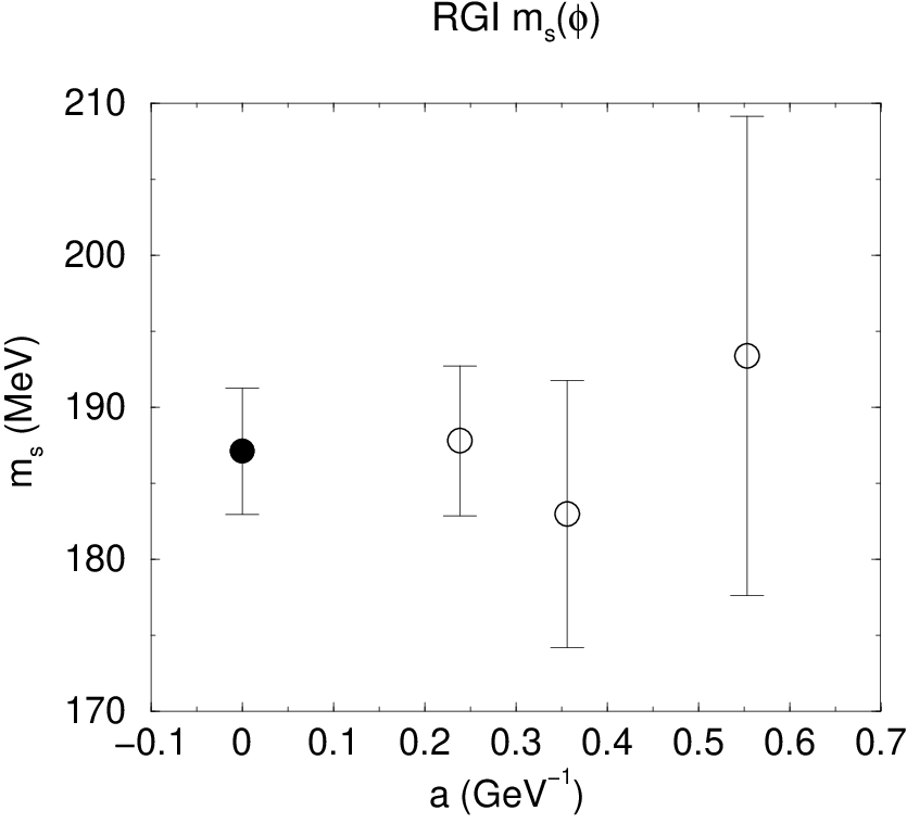
where four loop expression is used for renormalization group functions $\beta$ and $\tau$ in the $\overline{\rm MS}$ scheme[30, 38]. The results in Fig. 21 show good scalings, and the constant continuum extrapolations give

	$\displaystyle{m}_{ud}^{\overline{\rm MS}}({\rm NDR},2{\rm GeV})=4.026(48)\;({\rm MeV}),$		(V.72)
	$\displaystyle{m}_{s}^{\overline{\rm MS}}(K)({\rm NDR},2{\rm GeV})=105.6(12)\;({\rm MeV}),$		(V.73)
	$\displaystyle{m}_{s}^{\overline{\rm MS}}(\phi)({\rm NDR},2{\rm GeV})=134.2(30)\;({\rm MeV}).$		(V.74)

Contrary to the case of $B_{K}$ , perturbatively renormalized quark masses of the previous CP-PACS result (filled squares) are underestimated, as seen in the figure. This clearly shows that the necessity of the non-perturbative renormalization for precision calculations in lattice QCD. We think that the large effects of the renormalizations are mainly canceled in the ratio of the $B_{K}$ definition, and therefore, such cancellations can not be expected for general operators.

VI Conclusion and Discussions

In this paper we have performed the non-perturbative renormalization of $B_{K}$ and quark masses in the quenched domain-wall QCD using the Schrödinger functional method. Combined with the non-perturbative running obtained by Alpha collaboration, we have obtained the renormalization factors, which convert the lattice bare $B_{K}$ and quark masses previously obtained by the CP-PACS collaboration to the RGI values. We obtain

	$\displaystyle\widehat{B}_{K}=0.782(5)(7),$		(VI.75)
	$\displaystyle\hat{m}_{ud}^{\rm RGI}=5.613(66)\;({\rm MeV}),$		(VI.76)
	$\displaystyle\hat{m}_{s}^{\rm RGI}(K)=147.1(17)\;({\rm MeV}),$		(VI.77)
	$\displaystyle\hat{m}_{s}^{\rm RGI}(\phi)=187.1(41)\;({\rm MeV}).$		(VI.78)

in the continuum limit. These values correspond to renormalized values in $\overline{\rm MS}$ scheme with the naive dimensional regularization are given as

	$\displaystyle B_{K}^{\overline{\rm MS}}({\rm NDR},2{\rm GeV})=0.565(4)(5),$		(VI.79)
	$\displaystyle{m}_{ud}^{\overline{\rm MS}}({\rm NDR},2{\rm GeV})=4.026(48)\;({\rm MeV}),$		(VI.80)
	$\displaystyle{m}_{s}^{\overline{\rm MS}}(K)({\rm NDR},2{\rm GeV})=105.6(12)\;({\rm MeV}),$		(VI.81)
	$\displaystyle{m}_{s}^{\overline{\rm MS}}(\phi)({\rm NDR},2{\rm GeV})=134.2(30)\;({\rm MeV}).$		(VI.82)

With the non-perturbative renormalization in the DWQCD and data at $a^{-1}\simeq 2,3,4$ GeV, we can extract $B_{K}$ within 2% errors, except the quenching errors. The error in $B_{K}$ is directly reflected to that in the CKM triangle constraint from $\epsilon_{K}$ . If we adopt our $B_{K}$ for an input, the error of the constraint is improved as is shown in Fig. 22. The solid lines are central value and one standard deviation of the constraint from $\epsilon_{K}$ with our $B_{K}$ . The dashed lines are results with $B_{K}$ adopted by the CKM fitter group [42]. For other inputs we used those given by the CKM fitter. ^†^† † We use the standard formula for $\epsilon_{K}$ as is given in Ref. [42]. Note however that our figure is not a global fit.

Although the perturbative renormalization can also achieve the same level of accuracy for $B_{K}$ , it is clearly shown that the nonperturbative renormalization is indeed necessary for the precise determination of quark masses in lattice QCD.

Acknowledgments

This work is supported in part by Grants-in-Aid of the Ministry of Education (NO.15540251, 13135204, 18740130).

References

[1] T. Blum and A. Soni, Phys. Rev. D 56 (1997) 174 [arXiv:hep-lat/9611030].
[2] T. Blum and A. Soni, Phys. Rev. Lett. 79 (1997) 3595 [arXiv:hep-lat/9706023].
[3] S. Aoki et al. [JLQCD Collaboration], Phys. Rev. Lett. 80 (1998) 5271. [arXiv:hep-lat/9710073].
[4] S. Aoki et al. [JLQCD Collaboration], Phys. Rev. Lett. 81 (1998) 1778 [arXiv:hep-lat/9705035].
[5] S. Aoki et al. [JLQCD Collaboration], Phys. Rev. D 60 (1999) 034511 [arXiv:hep-lat/9901018].
[6] A. Ali Khan et al. [CP-PACS Collaboration], Phys. Rev. D 64 (2001) 114506. [arXiv:hep-lat/0105020].
[7] N. Garron, L. Giusti, C. Hoelbling, L. Lellouch and C. Rebbi, Phys. Rev. Lett. 92 (2004) 042001 [arXiv:hep-ph/0306295].
[8] T. A. DeGrand [MILC Collaboration], Phys. Rev. D 69 (2004) 014504 [arXiv:hep-lat/0309026].
[9] D. Becirevic, Ph. Boucaud, V. Gimenez, V. Lubicz and M. Papinutto, Eur. Phys. J. C 37 (2004) 315 [arXiv:hep-lat/0407004].
[10] W. Lee, T. Bhattacharya, G. T. Fleming, R. Gupta, G. Kilcup and S. R. Sharpe, Phys. Rev. D 71 (2005) 094501 [arXiv:hep-lat/0409047].
[11] Y. Aoki et al., Phys. Rev. D 73 (2006) 094507. [arXiv:hep-lat/0508011].
[12] P. Dimopoulos, J. Heitger, F. Palombi, C. Pena, S. Sint and A. Vladikas [ALPHA Collaboration], Nucl. Phys. B 749 (2006) 69 [arXiv:hep-ph/0601002].
[13] P. Dimopoulos, J. Heitger, F. Palombi, C. Pena, S. Sint and A. Vladikas, Nucl. Phys. B 776 (2007) 258 [arXiv:hep-lat/0702017].
[14] M. Lüscher, R. Narayanan, P. Weisz and U. Wolff, Nucl. Phys. B 384 (1992) 168 [arXiv:hep-lat/9207009].
[15] M. Lüscher, S. Sint, R. Sommer and P. Weisz Nucl. Phys. B 478 (1996) 365 [arXiv:hep-lat/9605038].
[16] M. Lüscher and P. Weisz, Nucl. Phys. B 479 (1996) 429 [arXiv:hep-lat/9606016].
[17] S. Sint, Nucl. Phys. Proc. Suppl. 94 (2001) 79 [arXiv:hep-lat/0011081]. and references there in.
[18] ALPHA Collaboration, M. Guagnelli et al. JHEP 0603 (2006) 088. [arXiv:hep-lat/0505002].
[19] F. Palombi, C. Pena and S. Sint, JHEP 0603 (2006) 089. [arXiv:hep-lat/0505003].
[20] S. Aoki et al. [CP-PACS Collaboration], Phys. Rev. D70 (2004) 034503 [arXiv:hep-lat/0312011].
[21] M. Lüscher, S. Sint, R. Sommer and H. Wittig, Nucl. Phys. B 491 (1997) 344 [arXiv:hep-lat/9611015].
[22] Y. Iwasaki, preprint, UTHEP-118 (Dec. 1983), unpublished.
[23] S. Takeda, S. Aoki and K. Ide, Phys. Rev. D 68 (2003) 014505 [arXiv:hep-lat/0304013].
[24] CP-PACS Collaboration, S. Takeda et al., Phys. Rev. D70 (2004) 074510 [arXiv:hep-lat/0408010].
[25] Y. Taniguchi, JHEP 0512 (2005) 037 [arXiv:hep-lat/0412024].
[26] Y. Taniguchi, arXiv:hep-lat/0507008.
[27] Y. Taniguchi, JHEP 0610 (2006) 027. [arXiv:hep-lat/0604002].
[28] Y. Shamir, Nucl. Phys. B 406 (1993) 90 [arXiv:hep-lat/9303005].
[29] V. Furman and Y. Shamir, Nucl. Phys. B 439, 54 (1995) [arXiv:hep-lat/9405004].
[30] T. van Ritbergen, J. A. M. Vermaseren and S. A. Larin, Phys. Lett. B 400 (1997) 379 [arXiv:hep-ph/9701390].
[31] A. J. Buras and P. H. Weisz, Nucl. Phys. B 333 (1990) 66.
[32] S. Necco and R. Sommer, Nucl. Phys. B 622 (2002) 328 [arXiv:hep-lat/0108008].
[33] S. Aoki, T. Izubuchi, Y. Kuramashi and Y. Taniguchi, Phys. Rev. D 59 (1999) 094505 [arXiv:hep-lat/9810020].
[34] S. Aoki, T. Izubuchi, Y. Kuramashi and Y. Taniguchi, Phys. Rev. D 60 (1999) 114504 [arXiv:hep-lat/9902008].
[35] S. Aoki, T. Izubuchi, Y. Kuramashi and Y. Taniguchi, Phys. Rev. D 67 (2003) 094502 [arXiv:hep-lat/0206013].
[36] S. Sint and P. Weisz [ALPHA collaboration], Nucl. Phys. B 545 (1999) 529 [arXiv:hep-lat/9808013].
[37] S. Capitani, M. Lüscher, R. Sommer and H. Wittig [ALPHA Collaboration], Nucl. Phys. B 544 (1999) 669 [arXiv:hep-lat/9810063].
[38] K. G. Chetyrkin and A. Retey, Nucl. Phys. B 583 (2000) 3 [arXiv:hep-ph/9910332].
[39] S. Aoki et al. [CP-PACS Collaboration], Phys. Rev. Lett. 84 (2000) 238 [arXiv:hep-lat/9904012].
[40] A. Ali Khan et al. [CP-PACS Collaboration], Phys. Rev. Lett. 85 (2000) 4674 [Erratum-ibid. 90 (2003) 029902] [arXiv:hep-lat/0004010].
[41] S. Aoki et al. [JLQCD Collaboration], Phys. Rev. Lett. 82 (1999) 4392 [arXiv:hep-lat/9901019].
[42] J. Charles et al. [CKMfitter Group], Eur. Phys. J. C 41 (2005) 1 [arXiv:hep-ph/0406184].

Appendix A Chiral Ward-Takahashi identity for SF formalism with DWF

In this appendix we derive the Ward-Takahashi identity (IV.58) for the Schrödinger functional formalism with domain-wall fermion. An explicit form of the chirally rotated correlation function used for evaluation of $Z_{VV+AA}$ is presented. We use the same notation of Ref. [27] for the SF formalism in this appendix.

In this paper we adopt following massless DWF action with an orbifolding projection

	$\displaystyle S_{\rm dwf}^{\rm SF}=a^{4}\sum\frac{1}{2}{\overline{\psi}}{\overline{\Pi}}_{+}D_{\rm dwf}\psi$		(A.83)
	$\displaystyle{\overline{\Pi}}_{\pm}=\frac{1\pm\gamma_{0}\gamma_{5}PQR}{2}.$		(A.84)

Here $P$ is a parity transformation in fifth direction $P_{s,t}\psi(\vec{x},x_{0},t)=\psi(\vec{x},x_{0},N_{5}-s+1)$ , and $R$ is a time reflection operator acting on the temporal direction $R_{x_{0},y_{0}}\psi(\vec{x},y_{0},s)=\psi(\vec{x},-x_{0},s)$ . $Q$ is the vector charge matrix for the chiral transformation [29]

\displaystyle Q_{s,t}=\begin{pmatrix}1&0&0&0&0&0\cr 0&1&0&0&0&0\cr 0&0&1&0&0&0\cr 0&0&0&-1&0&0\cr 0&0&0&0&-1&0\cr 0&0&0&0&0&-1\cr\end{pmatrix},\quad({\rm for}\;N_{5}=6).

(A.85)

For this action the physical quark propagator is given by

\displaystyle G_{\rm quark}^{\rm SF}(x,y)=2(G_{\rm quark}\Pi_{+})_{x,y},\quad\Pi_{\pm}=\frac{1\pm\gamma_{0}R}{2}.

(A.86)

This propagator is shown to agree with (III.37) numerically and we employ the latter in our numerical simulations.

We consider the chiral rotation of the first flavour

\displaystyle\psi_{1}(x,s)\to\widetilde{\psi}_{1}(x,s)=\left(e^{-i\alpha Q}\right)_{st}{\psi}_{1}(x,t),\quad{\overline{\psi}}_{1}(x,s)\to\widetilde{{\overline{\psi}}}_{1}(x,s)={{\overline{\psi}}}_{1}(x,t)\left(e^{i\alpha Q}\right)_{ts},

(A.87)

under which the physical quark and boundary quark fields are rotated as

	$\displaystyle\widetilde{q}_{1}(x)=e^{i\alpha\gamma_{5}}{q}_{1}(x),\quad\widetilde{{\overline{q}}}_{1}(x)={{\overline{q}}}_{1}(x)e^{i\alpha\gamma_{5}},$		(A.88)
	$\displaystyle\widetilde{\zeta}_{1}(x)=e^{-i\alpha\gamma_{5}}{\zeta}_{1}(x),\quad\widetilde{\overline{\zeta}}_{1}(x)={\overline{\zeta}}_{1}(x)e^{-i\alpha\gamma_{5}},$		(A.89)
	$\displaystyle\widetilde{\zeta}^{\prime}_{1}(x)=e^{-i\alpha\gamma_{5}}{\zeta}^{\prime}_{1}(x),\quad\widetilde{\overline{\zeta}}^{\prime}_{1}(x)={\overline{\zeta}}^{\prime}_{1}(x)e^{-i\alpha\gamma_{5}}.$		(A.90)

For $\alpha=\pi/2$ the action for the first flavour is transformed as

	$\displaystyle S_{\rm dwf}^{\rm SF}\to\widetilde{S}_{\rm dwf}^{\rm SF}+Y,$		(A.91)
	$\displaystyle\widetilde{S}_{\rm dwf}^{\rm SF}=a^{4}\sum\frac{1}{2}\widetilde{{\overline{\psi}}}{{\overline{\Pi}}}_{-}{D}_{\rm dwf}\widetilde{\psi},$		(A.92)
	$\displaystyle Y=a^{4}\sum\widetilde{{\overline{\psi}}}{{\overline{\Pi}}}_{-}X\widetilde{\psi},$		(A.93)
	$\displaystyle aX=\left(P_{L}\delta_{s,\frac{N_{5}}{2}}\delta_{t,\frac{N_{5}}{2}+1}+P_{R}\delta_{s,\frac{N_{5}}{2}+1}\delta_{t,\frac{N_{5}}{2}}\right)\delta_{x,y}.$		(A.94)

We notice that the orbifolding projection in the rotated action $\widetilde{S}_{\rm dwf}^{\rm SF}$ has an opposite sign and the rotated quark fields satisfy the opposite Dirichlet boundary condition to (III.39)

	$\displaystyle P_{-}\widetilde{q}_{1}(x)\|_{x_{0}=0}=0,\quad P_{+}\widetilde{q}_{1}(x)\|_{x_{0}=N_{T}}=0,$		(A.95)
	$\displaystyle\widetilde{{\overline{q}}}_{1}(x)P_{+}\|_{x_{0}=0}=0,\quad\widetilde{{\overline{q}}}_{1}(x)P_{-}\|_{x_{0}=N_{T}}=0.$		(A.96)

Now we derive the Ward-Takahashi identity for the four point function (II.18) and two point functions (II.23) as

$\displaystyle\mathcal{F}_{\Gamma_{A}\Gamma_{B}\Gamma_{C}}^{\pm}$	$\displaystyle=$	$\displaystyle\frac{1}{L^{3}}\langle\mathcal{O}_{21}[\Gamma_{A}]\mathcal{O}_{45}[\Gamma_{B}]O_{VA+AV}^{\pm}(x)\mathcal{O}^{\prime}_{53}[\Gamma_{C}]\rangle_{S}$	(A.97)
	$\displaystyle=$	$\displaystyle\frac{1}{L^{3}}\langle\widetilde{\mathcal{O}}_{21}[\Gamma_{A}i\gamma_{5}]\mathcal{O}_{45}[\Gamma_{B}]i\widetilde{O}_{VV+AA}^{\pm}(x)\mathcal{O}^{\prime}_{53}[\Gamma_{C}]\rangle_{\tilde{S}+Y},$	(A.97)
$\displaystyle f_{1}$	$\displaystyle=$	$\displaystyle-\frac{1}{2L^{6}}\langle\mathcal{O}_{12}^{\prime}[\gamma_{5}]\mathcal{O}_{21}[\gamma_{5}]\rangle_{S}=-\frac{1}{2L^{6}}\langle i\widetilde{\mathcal{O}}_{12}^{\prime}[1]i\widetilde{\mathcal{O}}_{21}[1]\rangle_{\tilde{S}+Y},$	(A.98)
$\displaystyle k_{1}$	$\displaystyle=$	$\displaystyle-\frac{1}{6L^{6}}\sum_{k=1}^{3}\langle\mathcal{O}^{\prime}_{12}[\gamma_{k}]\mathcal{O}_{21}[\gamma_{k}]\rangle_{S}=-\frac{1}{6L^{6}}\sum_{k=1}^{3}\langle\widetilde{\mathcal{O}}^{\prime}_{12}[i\gamma_{5}\gamma_{k}]\widetilde{\mathcal{O}}_{21}[\gamma_{k}i\gamma_{5}]\rangle_{\tilde{S}+Y},$	(A.99)

where

	$\displaystyle\widetilde{O}^{\pm}_{VV+AA}$	$\displaystyle=$	$\displaystyle\left(\widetilde{{\overline{q}}}_{1}\gamma_{\mu}q_{2}\right)\left({\overline{q}}_{3}\gamma_{\mu}q_{4}\right)+\left(\widetilde{{\overline{q}}}_{1}\gamma_{\mu}\gamma_{5}q_{2}\right)\left({\overline{q}}_{3}\gamma_{\mu}\gamma_{5}q_{4}\right)$		(A.100)
			$\displaystyle\pm\left\{\left(\widetilde{{\overline{q}}}_{1}\gamma_{\mu}q_{4}\right)\left({\overline{q}}_{3}\gamma_{\mu}q_{2}\right)+\left(\widetilde{{\overline{q}}}_{1}\gamma_{\mu}\gamma_{5}q_{4}\right)\left({\overline{q}}_{3}\gamma_{\mu}\gamma_{5}q_{2}\right)\right\}.$		(A.100)

Operators with tilde consist of the chirally rotated field for the first flavour, which satisfies the opposite SF Dirichlet boundary condition. Subscript $S$ and $\tilde{S}+Y$ mean the action under which the VEV is taken.

The chiral symmetry breaking effect comes from a contribution of $Y$ on the right hand side of the WT identity, which generates an operator mixing with the parity even operator. The contribution should be suppressed exponentially in the physical quark propagator and this is the case at tree level. We evaluate the effect by comparing two correlation functions directly

\displaystyle\langle\mathcal{O}_{21}[\Gamma_{A}]\mathcal{O}_{45}[\Gamma_{B}]O_{VA+AV}^{\pm}(x)\mathcal{O}^{\prime}_{53}[\Gamma_{C}]\rangle_{S}\leftrightarrow\langle\widetilde{\mathcal{O}}_{21}[\Gamma_{A}i\gamma_{5}]\mathcal{O}_{45}[\Gamma_{B}]i\widetilde{O}_{VV+AA}^{\pm}(x)\mathcal{O}^{\prime}_{53}[\Gamma_{C}]\rangle_{\tilde{S}}.

(A.101)

For this purpose we define the renormalization factor for the parity even four fermi operator as

	$\displaystyle Z_{VV+AA;s}^{\pm}(g_{0},a\mu)=\frac{\widetilde{h}_{s}^{\pm({\rm tree})}(x_{0}=L/2)}{\widetilde{h}_{s}^{\pm}(x_{0}=L/2;g_{0})},$		(A.102)
	$\displaystyle\widetilde{h}_{1}^{\pm}(x_{0})=\frac{\widetilde{\mathcal{F}}_{\gamma_{5},\gamma_{5},\gamma_{5}}^{\pm}(x_{0})}{\widetilde{f}_{1}^{3/2}},$		(A.103)
	$\displaystyle\widetilde{\mathcal{F}}_{\Gamma_{A}\Gamma_{B}\Gamma_{C}}^{\pm}(x_{0})=\frac{1}{L^{3}}\langle\widetilde{\mathcal{O}}_{21}[\Gamma_{A}i\gamma_{5}]\mathcal{O}_{45}[\Gamma_{B}]i\widetilde{O}_{VV+AA}^{\pm}(x)\mathcal{O}^{\prime}_{53}[\Gamma_{C}]\rangle_{\tilde{S}},$		(A.104)
	$\displaystyle\widetilde{f}_{1}=-\frac{1}{2L^{6}}\langle i\widetilde{\mathcal{O}}_{12}^{\prime}[1]i\widetilde{\mathcal{O}}_{21}[1]\rangle_{\tilde{S}}$		(A.105)

and compare it with that for the parity odd operator.

Appendix B Numerical analysis of $B_{K}$ for $\beta=3.2$

Since the numerical data of CP-PACS collaboration at $\beta=3.2$ is new and not published, we give a short summary of its numerical analysis in this appendix.

B.1 Run parameters and measurements

We carry out run at $\beta=3.2$ , corresponding to a lattice spacing $a^{-1}=4.19(6)$ GeV determined from the the $\rho$ meson mass $m_{\rho}=770$ MeV. We use the lattice size $N_{\sigma}^{3}\times N_{t}\times N_{5}=48^{3}\times 80\times 16$ . This lattice has a reasonably large spatial size of $aN_{\sigma}\approx 2.3$ fm and fifth dimensional length $N_{5}=16$ , which has been confirmed to be enough for $B_{K}$ [6]. In this numerical simulation the domain wall height is taken to be $M=1.8$ .

We take degenerate quarks in our calculations. The value of bare quark mass is chosen to be $m_{f}a=0.009,0.018,0.027,0.036$ , which covers the range that $m_{PS}/m_{V}\approx 0.5334-0.8224$ .

Quenched gauge configurations are generated on four-dimensional lattices. A sweep of gauge update contains one pseudo-heatbath and four overrelaxation steps. After a thermalization of 2000 sweeps hadron propagators and 3-point functions necessary to evaluate $B_{K}$ are calculated at every 200th sweep. The gauge configuration on each fifth dimensional coordinate $s$ is identical and is fixed to the Coulomb gauge.

The domain-wall quark propagator needed to extract the $B_{K}$ is calculated by the conjugate gradient algorithm with an even-odd pre-conditioning. Two quark propagators are evaluated for each configuration corresponding to the wall sources placed at either $t=4$ or $77$ in the time direction with the Dirichlet boundary condition, while the periodic boundary condition is imposed in the spatial directions. The two quark propagators are combined to form the kaon Green function with an insertion of the four-quark operator at time slices $1\leq t\leq N_{t}$ in a standard manner. We employ the same quark propagators to evaluate pseudoscalar and vector meson propagators, and extract their masses.

B.2 Pseudo scalar and vector meson masses

We extract pseudoscalar and vector meson masses $m_{PS}$ and $m_{V}$ at each $m_{f}$ by a single exponential fit with meson propagators. Representative plots of effective masses are shown in Figs. 23 and 24. Fitting ranges chosen from inspection of such plots are $24\leq t\leq 55$ and $14\leq t\leq 30$ for pseudoscalar and vector meson masses, respectively.

For the chiral extrapolation we fit $m_{PS}^{2}$ and $m_{V}$ linearly in $m_{f}a$ as illustrated in Fig. 25. Since pseudoscalar meson mass does not vanish at $m_{f}=0$ , we employ a fit of the form

	$\displaystyle m_{PS}^{2}a^{2}$	$\displaystyle=$	$\displaystyle A_{PS}(m_{f}a+m_{\rm res}a),$		(B.106)
	$\displaystyle m_{V}a$	$\displaystyle=$	$\displaystyle A_{V}+B_{V}m_{f}a$		(B.107)

and determine the parameters $A_{PS},m_{\rm res}a$ for the pseudoscalar meson, and $A_{V},B_{V}$ for the vector meson. The physical bare masses, $m_{f}^{ud}$ for the generated $u$ and $d$ quarks and $m_{f}^{s}$ for the $s$ quark are determined by equations that

$\displaystyle\frac{\sqrt{A_{PS}(m_{f}^{ud}a+m_{\rm res}a)}}{A_{V}+B_{V}m_{f}^{ud}a}$	$\displaystyle=$	$\displaystyle\frac{m_{\pi}}{m_{\rho}}=\frac{0.135}{0.77},$	(B.108)
$\displaystyle\frac{\sqrt{A_{PS}\left((m_{f}^{s}(K)a+m_{f}^{ud}a)/2+m_{\rm res}a\right)}}{A_{V}+B_{V}m_{f}^{ud}a}$	$\displaystyle=$	$\displaystyle\frac{m_{K}}{m_{\rho}}=\frac{0.495}{0.77},$	(B.109)
$\displaystyle\frac{A_{V}+B_{V}m_{f}^{s}(\phi)a}{A_{V}+B_{V}m_{f}^{ud}a}$	$\displaystyle=$	$\displaystyle\frac{m_{\phi}}{m_{\rho}}=\frac{1.0194}{0.77}.$	(B.110)

For the $s$ quark, we extract two values of the $s$ quark mass, $m_{f}^{s}(K)$ from the kaon mass input or $m_{f}^{s}(\phi)$ from the phi meson mass input. We then fix the lattice spacing $a$ by setting the vector meson mass at the physical quark mass point $m_{f}^{ud}$ to the experimental value $m_{\rho}=770$ MeV. Numerical values of lattice spacing and quark masses are listed in table 1.

B.3 Extraction of $B$ parameters

In the course of our simulation we measure the kaon $B_{K}$ (I.2). The $s$ and $d$ quark fields defining $B_{K}$ are the physical fields given by (III.35), and the four-quark and bilinear operators are taken to be local in the 4-dimensional space-time.

In Fig. 26 we show typical data for the ratio of kaon Green functions for $B_{K}$ as a function of the temporal site $t$ of the weak operator. The values of these quantities at each $m_{f}$ are extracted by fitting the plateau with a constant. The fitting range, determined by the inspection of plots for the ratio and those for the effective pseudo scalar meson mass, is $24\leq t\leq 55$ .

The bare value of $B_{K}$ is interpolated as a function of $m_{f}a$ using a formula suggested by chiral perturbation theory,

\displaystyle B_{K}=B\left(1-3c\ m_{f}a\ \log(m_{f}a)+b\ m_{f}a\right).

(B.111)

This interpolation is illustrated in Fig. 27. The physical value of $B_{K}$ is obtained at the point $m_{f}=(m_{f}^{s}(K)+m_{f}^{ud})/2$ estimated from the experimental value of $m_{K}/m_{\rho}$ (a solid circle in Fig. 27). The result is given in table 1.

$\beta$	$2.6$	$2.9$	$3.2$
$B_{K}^{(0)}$	$0.5908(57)$	$0.5655(69)$	$0.5478(71)$
$a^{-1}$ (GeV)	$1.807(37)$	$2.807(55)$	$4.186(65)$
${m}_{ud}$ (MeV)	$0.40(34)$	$1.85(50)$	$4.65(52)$
${m}_{ud}+{m}_{\rm res}$ (MeV)	$3.306(68)$	$3.226(72)$	$3.216(52)$
${m}_{s}(K)$ (MeV)	$83.8(19)$	$83.2(20)$	$85.8(14)$
${m}_{s}(K)+{m}_{\rm res}$ (MeV)	$86.7(18)$	$84.6(19)$	$84.3(14)$
${m}_{s}(\phi)$	$114.1(93)$ (MeV)	$104.6(50)$	$107.8(27)$

Table 1: Numerical values of bare

B_{K}

in DWQCD given by CP-PACS collaboration [6]. Values of lattice spacing and bare quark masses are also listed. Here

m_{ud}

is the

u,d

quark mass from the

\pi

input,

m_{s}(K/\phi)

is the strange quark mass from the

K

(\phi)

input, and

-m_{\rm res}

is a residual quark mass where the pion mass vanishes. Data at

\beta=3.2

is new and not published in Ref. [6].

$N_{L}$	$6$	$8$	$10$	$12$	$14$	$16$	$18$	$20$
$\beta$	$2.4446$	$2.6339$	$2.7873$	$2.9175$	$3.0313$	$3.1331$	$3.2254$	$3.3103$
num. of conf. for scheme $1\sim 5$	$5165$	$3632$	$2000$	$2188$	$1000$	$868$	$778$	$104$
num. of conf. for scheme $6\sim 9$	$1165$	$1032$	$1000$	$670$	$284$	$312$	$200$	$104$

Table 2: Values of

\beta

which satisfies

aN_{T}=2L_{\rm max}

and number of configurations for each lattice size. Data at

N_{L}=20

is used only for the step scaling function.

$N_{L}$	$6$	$8$	$10$	$12$	$14$	$16$	$18$
$\beta$	$2.4446$	$2.6339$	$2.7873$	$2.9175$	$3.0313$	$3.1331$	$3.2254$
$Z_{V}$	$0.79580(23)$	$0.85837(18)$	$0.87048(15)$	$0.90395(12)$	$0.92286(30)$	$0.94463(13)$	$0.96184(12)$
$Z_{VA;1}^{+}$	$0.69767(89)$	$0.8778(14)$	$0.9189(18)$	$1.0179(21)$	$1.0785(34)$	$1.1388(37)$	$1.1821(44)$
$Z_{VA;2}^{+}$	$0.7196(13)$	$0.9089(21)$	$0.9679(28)$	$1.0758(31)$	$1.1521(53)$	$1.2132(59)$	$1.264(18)$
$Z_{VA;3}^{+}$	$0.7398(11)$	$0.9439(18)$	$0.9956(23)$	$1.1088(26)$	$1.1804(44)$	$1.2484(48)$	$1.2994(58)$
$Z_{VA;4}^{+}$	$0.6850(11)$	$0.8528(17)$	$0.9030(23)$	$0.9982(24)$	$1.0648(40)$	$1.1196(45)$	$1.1645(54)$
$Z_{VA;5}^{+}$	$0.6819(11)$	$0.8489(18)$	$0.8985(23)$	$0.9933(25)$	$1.0595(42)$	$1.1138(47)$	$1.157(16)$
$Z_{VA;6}^{+}$	$0.6382(18)$	$0.7812(25)$	$0.8224(26)$	$0.8980(35)$	$0.9592(53)$	$1.0093(56)$	$1.039(31)$
$Z_{VA;7}^{+}$	$0.6817(16)$	$0.8541(21)$	$0.8930(23)$	$0.9822(31)$	$1.0450(49)$	$1.1058(49)$	$1.1409(66)$
$Z_{VA;8}^{+}$	$0.6319(17)$	$0.7702(23)$	$0.8103(24)$	$0.8838(32)$	$0.9422(48)$	$0.9913(50)$	$1.0202(65)$
$Z_{VA;9}^{+}$	$0.6292(18)$	$0.7668(25)$	$0.8061(26)$	$0.8785(34)$	$0.9395(51)$	$0.9859(55)$	$1.015(28)$
$Z_{VA;1}^{-}$	$0.61284(68)$	$0.7101(11)$	$0.7024(13)$	$0.7472(15)$	$0.7587(25)$	$0.7886(25)$	$0.8061(30)$
$Z_{VA;2}^{-}$	$0.6677(14)$	$0.7791(22)$	$0.7937(28)$	$0.8516(28)$	$0.8820(48)$	$0.9074(53)$	$0.934(13)$
$Z_{VA;3}^{-}$	$0.69325(88)$	$0.8290(15)$	$0.8301(18)$	$0.8945(20)$	$0.9152(33)$	$0.9532(35)$	$0.9783(41)$
$Z_{VA;4}^{-}$	$0.6082(11)$	$0.6931(17)$	$0.6974(21)$	$0.7413(21)$	$0.7630(35)$	$0.7837(38)$	$0.8019(42)$
$Z_{VA;5}^{-}$	$0.6074(11)$	$0.6910(17)$	$0.6968(21)$	$0.7400(20)$	$0.7627(34)$	$0.7823(38)$	$0.802(10)$
$Z_{VA;6}^{-}$	$0.5924(21)$	$0.6679(28)$	$0.6726(27)$	$0.7135(36)$	$0.7295(55)$	$0.7537(56)$	$0.769(23)$
$Z_{VA;7}^{-}$	$0.6391(13)$	$0.7506(20)$	$0.7433(19)$	$0.7958(27)$	$0.8089(44)$	$0.8418(44)$	$0.8618(55)$
$Z_{VA;8}^{-}$	$0.5614(19)$	$0.6245(25)$	$0.6244(24)$	$0.6572(32)$	$0.6698(48)$	$0.6921(50)$	$0.7018(55)$
$Z_{VA;9}^{-}$	$0.5608(19)$	$0.6233(25)$	$0.6235(24)$	$0.6570(32)$	$0.6706(48)$	$0.6909(50)$	$0.703(19)$
$Z_{B_{K};1}$	$1.1017(12)$	$1.1914(19)$	$1.2127(24)$	$1.2457(25)$	$1.2663(40)$	$1.2763(42)$	$1.2778(47)$
$Z_{B_{K};2}$	$1.1363(18)$	$1.2336(28)$	$1.2774(37)$	$1.3166(38)$	$1.3527(63)$	$1.3596(66)$	$1.366(19)$
$Z_{B_{K};3}$	$1.1682(15)$	$1.2811(24)$	$1.3139(30)$	$1.3570(32)$	$1.3860(52)$	$1.3991(55)$	$1.4045(63)$
$Z_{B_{K};4}$	$1.0816(15)$	$1.1574(23)$	$1.1918(29)$	$1.2216(30)$	$1.2502(48)$	$1.2547(50)$	$1.2587(58)$
$Z_{B_{K};5}$	$1.0768(15)$	$1.1521(23)$	$1.1857(30)$	$1.2157(30)$	$1.2441(50)$	$1.2482(53)$	$1.251(17)$
$Z_{B_{K};6}$	$1.0084(23)$	$1.0605(32)$	$1.0854(34)$	$1.0990(42)$	$1.1285(62)$	$1.1313(62)$	$1.123(33)$
$Z_{B_{K};7}$	$1.0772(20)$	$1.1594(27)$	$1.1787(30)$	$1.2021(37)$	$1.2294(57)$	$1.2394(55)$	$1.2329(72)$
$Z_{B_{K};8}$	$0.9984(22)$	$1.0456(30)$	$1.0695(31)$	$1.0817(39)$	$1.1086(56)$	$1.1111(56)$	$1.1025(71)$
$Z_{B_{K};9}$	$0.9942(23)$	$1.0410(32)$	$1.0640(33)$	$1.0752(41)$	$1.1054(60)$	$1.1050(61)$	$1.097(30)$
$Z_{P}$	$0.65512(64)$	$0.66259(88)$	$0.64990(99)$	$0.6560(10)$	$0.6580(16)$	$0.6606(16)$	$0.6627(18)$
$Z_{m}$	$1.5264(15)$	$1.5092(20)$	$1.5387(23)$	$1.5244(24)$	$1.5198(37)$	$1.5137(37)$	$1.5091(42)$

Table 3: Numerical values of

Z_{V}(g_{0})

Z_{VA+AV;s}^{\pm}(g_{0},a\mu_{\rm min})

and

Z_{B_{K};s}(g_{0},a\mu_{\rm min})

2L_{\rm max}

. Values of

Z_{P}(g_{0},a\mu_{\rm min})

and

Z_{m}(g_{0},a\mu_{\rm min})

are also listed for the latter use.

$N_{L}$	$4$	$6$	$8$	$10$	$20$
$\beta$	$2.6339$	$2.9175$	$3.1331$	$3.3103$	$3.3103$
$Z_{V}$	$0.9905(21)$	$0.87148(98)$	$0.97930(77)$	$0.97587(57)$	$0.97898(26)$
$Z_{VA;1}^{+}$	$1.0784(69)$	$0.7937(48)$	$1.0967(59)$	$1.0853(70)$	$1.258(11)$
$Z_{VA;2}^{+}$	$1.0302(74)$	$0.8061(63)$	$1.0945(84)$	$1.1054(91)$	$1.349(16)$
$Z_{VA;3}^{+}$	$1.1000(72)$	$0.8215(56)$	$1.1446(67)$	$1.1384(83)$	$1.376(14)$
$Z_{VA;4}^{+}$	$1.0058(70)$	$0.7807(56)$	$1.0480(74)$	$1.0555(76)$	$1.246(12)$
$Z_{VA;5}^{+}$	$1.0076(71)$	$0.7811(57)$	$1.0498(77)$	$1.0555(76)$	$1.240(12)$
$Z_{VA;6}^{+}$	$1.0018(70)$	$0.7703(54)$	$1.0346(73)$	$1.0366(73)$	$1.1181(91)$
$Z_{VA;7}^{+}$	$1.0797(69)$	$0.7969(49)$	$1.1024(59)$	$1.0907(71)$	$1.2145(89)$
$Z_{VA;8}^{+}$	$0.9871(67)$	$0.7574(51)$	$1.0094(68)$	$1.0113(66)$	$1.0995(85)$
$Z_{VA;9}^{+}$	$0.9890(68)$	$0.7578(51)$	$1.0112(72)$	$1.0112(66)$	$1.0942(88)$
$Z_{VA;1}^{-}$	$1.0609(63)$	$0.7389(30)$	$0.9721(49)$	$0.9349(57)$	$0.8252(67)$
$Z_{VA;2}^{-}$	$0.9831(82)$	$0.7746(69)$	$0.9775(93)$	$0.9847(99)$	$0.971(15)$
$Z_{VA;3}^{-}$	$1.1135(69)$	$0.7933(42)$	$1.0644(60)$	$1.0334(74)$	$0.995(10)$
$Z_{VA;4}^{-}$	$0.9423(74)$	$0.7288(58)$	$0.9043(79)$	$0.9033(79)$	$0.842(11)$
$Z_{VA;5}^{-}$	$0.9435(74)$	$0.7329(57)$	$0.9088(79)$	$0.9070(75)$	$0.841(11)$
$Z_{VA;6}^{-}$	$0.9559(77)$	$0.7401(61)$	$0.9239(83)$	$0.9234(81)$	$0.805(11)$
$Z_{VA;7}^{-}$	$1.0929(66)$	$0.7696(37)$	$1.0252(54)$	$0.9901(65)$	$0.8777(72)$
$Z_{VA;8}^{-}$	$0.9248(71)$	$0.7070(53)$	$0.8710(73)$	$0.8654(70)$	$0.7430(93)$
$Z_{VA;9}^{-}$	$0.9260(71)$	$0.7110(54)$	$0.8753(74)$	$0.8690(67)$	$0.7425(93)$
$Z_{B_{K};1}$	$1.0992(51)$	$1.0450(53)$	$1.1436(61)$	$1.1397(73)$	$1.313(11)$
$Z_{B_{K};2}$	$1.0502(59)$	$1.0615(74)$	$1.1413(88)$	$1.1608(96)$	$1.407(17)$
$Z_{B_{K};3}$	$1.1213(55)$	$1.0816(63)$	$1.1935(71)$	$1.1954(87)$	$1.436(15)$
$Z_{B_{K};4}$	$1.0252(54)$	$1.0280(64)$	$1.0928(76)$	$1.1084(80)$	$1.300(13)$
$Z_{B_{K};5}$	$1.0271(55)$	$1.0285(65)$	$1.0947(80)$	$1.1084(81)$	$1.294(13)$
$Z_{B_{K};6}$	$1.0211(54)$	$1.0142(62)$	$1.0788(75)$	$1.0885(76)$	$1.1667(95)$
$Z_{B_{K};7}$	$1.1005(51)$	$1.0493(54)$	$1.1495(62)$	$1.1453(74)$	$1.2672(93)$
$Z_{B_{K};8}$	$1.0062(51)$	$0.9972(57)$	$1.0525(69)$	$1.0619(69)$	$1.1472(89)$
$Z_{B_{K};9}$	$1.0081(52)$	$0.9977(58)$	$1.0544(73)$	$1.0619(70)$	$1.1417(93)$
$Z_{P}$	$0.8718(36)$	$0.7680(33)$	$0.8160(36)$	$0.8051(37)$	$0.6712(53)$
$Z_{m}$	$1.1471(48)$	$1.3020(55)$	$1.2254(54)$	$1.2421(56)$	$1.490(12)$

Table 4: Numerical values of

Z_{V}(g_{0})

Z_{VA+AV;s}^{\pm}(g_{0},2a\mu_{\rm min})

Z_{B_{K};s}(g_{0},2a\mu_{\rm min})

Z_{P}(g_{0},2a\mu_{\rm min})

and

Z_{m}(g_{0},2a\mu_{\rm min})

L_{\rm max}

for SSF. A box size of

N_{L}=20

lattice is

2L_{\rm max}

$N_{L}$	$4$	$6$	$8$	$10$	$8$	$12$	$16$	$20$
$\beta$	$2.6339$	$2.9175$	$3.1331$	$3.3103$	$2.6339$	$2.9175$	$3.1331$	$3.3103$
$Z_{VA;1}^{+}$	$0.7664(38)$	$0.7669(49)$	$0.7928(54)$	$0.8157(50)$	$0.8778(14)$	$1.0179(21)$	$1.1388(37)$	$1.258(11)$
$Z_{VA;2}^{+}$	$0.7602(44)$	$0.7661(60)$	$0.7977(71)$	$0.8210(71)$	$0.9089(21)$	$1.0758(31)$	$1.2132(59)$	$1.349(16)$
$Z_{VA;3}^{+}$	$0.7829(39)$	$0.7937(55)$	$0.8260(62)$	$0.8629(96)$	$0.9439(18)$	$1.1088(26)$	$1.2484(48)$	$1.376(14)$
$Z_{VA;4}^{+}$	$0.7440(42)$	$0.7397(52)$	$0.7655(60)$	$0.801(14)$	$0.8528(17)$	$0.9982(24)$	$1.1196(45)$	$1.246(12)$
$Z_{VA;5}^{+}$	$0.7445(42)$	$0.7407(52)$	$0.7670(63)$	$0.802(14)$	$0.8489(18)$	$0.9933(25)$	$1.1138(47)$	$1.240(12)$
$Z_{VA;6}^{+}$	$0.7379(41)$	$0.7321(51)$	$0.7542(58)$	$0.7748(61)$	$0.7812(25)$	$0.8980(35)$	$1.0093(56)$	$1.1181(91)$
$Z_{VA;7}^{+}$	$0.7675(38)$	$0.7700(50)$	$0.7957(53)$	$0.8302(89)$	$0.8541(21)$	$0.9822(31)$	$1.1058(49)$	$1.2145(89)$
$Z_{VA;8}^{+}$	$0.7294(40)$	$0.7176(47)$	$0.7374(52)$	$0.771(13)$	$0.7702(23)$	$0.8838(32)$	$0.9913(50)$	$1.0995(85)$
$Z_{VA;9}^{+}$	$0.7298(41)$	$0.7186(48)$	$0.7389(56)$	$0.771(14)$	$0.7668(25)$	$0.8785(34)$	$0.9859(55)$	$1.0942(88)$
$Z_{VA;1}^{-}$	$0.8065(28)$	$0.7611(37)$	$0.7532(41)$	$0.7437(39)$	$0.7101(11)$	$0.7472(15)$	$0.7886(25)$	$0.8252(67)$
$Z_{VA;2}^{-}$	$0.8076(47)$	$0.7693(60)$	$0.7688(68)$	$0.7573(81)$	$0.7791(22)$	$0.8516(28)$	$0.9074(53)$	$0.971(15)$
$Z_{VA;3}^{-}$	$0.8465(34)$	$0.8193(48)$	$0.8221(52)$	$0.8241(92)$	$0.8290(15)$	$0.8945(20)$	$0.9532(35)$	$0.995(10)$
$Z_{VA;4}^{-}$	$0.7757(43)$	$0.7211(49)$	$0.7114(56)$	$0.711(13)$	$0.6931(17)$	$0.7413(21)$	$0.7837(38)$	$0.842(11)$
$Z_{VA;5}^{-}$	$0.7770(42)$	$0.7247(47)$	$0.7165(53)$	$0.717(13)$	$0.6910(17)$	$0.7400(20)$	$0.7823(38)$	$0.841(11)$
$Z_{VA;6}^{-}$	$0.7839(44)$	$0.7352(51)$	$0.7269(56)$	$0.7147(70)$	$0.6679(28)$	$0.7135(36)$	$0.7537(56)$	$0.805(11)$
$Z_{VA;7}^{-}$	$0.8299(32)$	$0.7948(44)$	$0.7920(45)$	$0.7929(85)$	$0.7506(20)$	$0.7958(27)$	$0.8418(44)$	$0.8777(72)$
$Z_{VA;8}^{-}$	$0.7605(41)$	$0.6996(45)$	$0.6854(50)$	$0.684(12)$	$0.6245(25)$	$0.6572(32)$	$0.6921(50)$	$0.7430(93)$
$Z_{VA;9}^{-}$	$0.7617(40)$	$0.7031(43)$	$0.6902(48)$	$0.690(12)$	$0.6233(25)$	$0.6570(32)$	$0.6909(50)$	$0.7425(93)$
$Z_{B_{K};1}$	$1.0096(33)$	$1.0715(63)$	$1.1041(69)$	$1.1221(66)$	$1.1914(19)$	$1.2457(25)$	$1.2763(42)$	$1.313(11)$
$Z_{B_{K};2}$	$1.0014(41)$	$1.0704(79)$	$1.1110(94)$	$1.1295(96)$	$1.2336(28)$	$1.3166(38)$	$1.3596(66)$	$1.407(17)$
$Z_{B_{K};3}$	$1.0314(36)$	$1.1089(72)$	$1.1504(81)$	$1.187(13)$	$1.2811(24)$	$1.3570(32)$	$1.3991(55)$	$1.436(15)$
$Z_{B_{K};4}$	$0.9801(38)$	$1.0334(67)$	$1.0661(78)$	$1.102(19)$	$1.1574(23)$	$1.2216(30)$	$1.2547(50)$	$1.300(13)$
$Z_{B_{K};5}$	$0.9807(39)$	$1.0348(68)$	$1.0683(83)$	$1.103(19)$	$1.1521(23)$	$1.2157(30)$	$1.2482(53)$	$1.294(13)$
$Z_{B_{K};6}$	$0.9721(37)$	$1.0228(65)$	$1.0504(76)$	$1.0659(82)$	$1.0605(32)$	$1.0990(42)$	$1.1313(62)$	$1.1667(95)$
$Z_{B_{K};7}$	$1.0112(33)$	$1.0758(63)$	$1.1082(68)$	$1.142(12)$	$1.1594(27)$	$1.2021(37)$	$1.2394(55)$	$1.2672(93)$
$Z_{B_{K};8}$	$0.9608(36)$	$1.0026(59)$	$1.0270(68)$	$1.060(18)$	$1.0456(30)$	$1.0817(39)$	$1.1111(56)$	$1.1472(89)$
$Z_{B_{K};9}$	$0.9615(37)$	$1.0040(60)$	$1.0291(73)$	$1.061(18)$	$1.0410(32)$	$1.0752(41)$	$1.1050(61)$	$1.1417(93)$
$Z_{P}$	$0.8277(22)$	$0.7670(30)$	$0.7394(35)$	$0.7240(31)$	$0.66259(88)$	$0.6560(10)$	$0.6606(16)$	$0.6712(53)$
$Z_{m}$	$1.2082(32)$	$1.3038(51)$	$1.3524(65)$	$1.3812(60)$	$1.5092(20)$	$1.5244(24)$	$1.5137(37)$	$1.490(12)$

Table 5: Numerical values of

Z_{VA+AV;s}^{\pm}(g_{0},a\mu)

Z_{B_{K};s}(g_{0},a\mu)

Z_{P}(g_{0},a\mu)

and

Z_{m}(g_{0},a\mu)

L_{\rm max}

and

2L_{\rm max}

M=1.4

for SSF.

$N_{L}$	$6$	$8$	$10$	$12$	$14$	$16$	$18$
$\beta$	$2.4446$	$2.6339$	$2.7873$	$2.9175$	$3.0313$	$3.1331$	$3.2254$
$Z_{V}$	$0.85609(24)$	$0.88162(19)$	$0.88822(16)$	$0.91166(12)$	$0.92852(30)$	$0.94719(13)$	$0.96359(12)$
$Z_{VA;1}^{+}$	$0.8285(11)$	$0.9344(15)$	$0.9645(19)$	$1.0392(21)$	$1.0951(34)$	$1.1470(37)$	$1.1880(44)$
$Z_{VA;2}^{+}$	$0.8546(15)$	$0.9675(23)$	$1.0160(30)$	$1.0983(32)$	$1.1698(53)$	$1.2218(59)$	$1.270(18)$
$Z_{VA;3}^{+}$	$0.8785(13)$	$1.0047(19)$	$1.0450(24)$	$1.1320(27)$	$1.1985(44)$	$1.2573(49)$	$1.3058(58)$
$Z_{VA;4}^{+}$	$0.8134(13)$	$0.9077(18)$	$0.9479(24)$	$1.0191(25)$	$1.0811(41)$	$1.1276(45)$	$1.1703(54)$
$Z_{VA;5}^{+}$	$0.8098(13)$	$0.9036(19)$	$0.9431(25)$	$1.0141(26)$	$1.0758(42)$	$1.1218(47)$	$1.163(16)$
$Z_{VA;6}^{+}$	$0.7582(21)$	$0.8317(26)$	$0.8634(28)$	$0.9169(35)$	$0.9741(53)$	$1.0166(56)$	$1.044(31)$
$Z_{VA;7}^{+}$	$0.8099(18)$	$0.9093(23)$	$0.9375(24)$	$1.0029(31)$	$1.0612(50)$	$1.1138(50)$	$1.1467(66)$
$Z_{VA;8}^{+}$	$0.7507(20)$	$0.8200(25)$	$0.8507(26)$	$0.9024(33)$	$0.9568(48)$	$0.9985(51)$	$1.0254(66)$
$Z_{VA;9}^{+}$	$0.7475(21)$	$0.8164(26)$	$0.8463(27)$	$0.8970(35)$	$0.9541(52)$	$0.9930(55)$	$1.020(28)$
$Z_{VA;1}^{-}$	$0.72775(80)$	$0.7558(12)$	$0.7373(14)$	$0.7628(16)$	$0.7704(25)$	$0.7942(26)$	$0.8101(30)$
$Z_{VA;2}^{-}$	$0.7929(17)$	$0.8293(23)$	$0.8331(29)$	$0.8694(29)$	$0.8956(48)$	$0.9139(53)$	$0.938(13)$
$Z_{VA;3}^{-}$	$0.8232(10)$	$0.8825(16)$	$0.8713(19)$	$0.9132(20)$	$0.9293(33)$	$0.9600(36)$	$0.9832(41)$
$Z_{VA;4}^{-}$	$0.7223(13)$	$0.7377(18)$	$0.7320(22)$	$0.7568(22)$	$0.7748(35)$	$0.7893(38)$	$0.8058(43)$
$Z_{VA;5}^{-}$	$0.7213(13)$	$0.7355(18)$	$0.7314(22)$	$0.7555(21)$	$0.7745(34)$	$0.7879(38)$	$0.806(10)$
$Z_{VA;6}^{-}$	$0.7038(24)$	$0.7111(30)$	$0.7061(29)$	$0.7285(36)$	$0.7408(56)$	$0.7592(56)$	$0.773(23)$
$Z_{VA;7}^{-}$	$0.7593(16)$	$0.7991(21)$	$0.7803(20)$	$0.8126(28)$	$0.8214(45)$	$0.8479(44)$	$0.8662(55)$
$Z_{VA;8}^{-}$	$0.6669(22)$	$0.6649(26)$	$0.6555(25)$	$0.6710(33)$	$0.6802(49)$	$0.6971(50)$	$0.7054(56)$
$Z_{VA;9}^{-}$	$0.6663(22)$	$0.6636(27)$	$0.6546(26)$	$0.6708(33)$	$0.6811(49)$	$0.6959(50)$	$0.706(19)$
$Z_{B_{K};1}$	$1.1304(12)$	$1.2021(19)$	$1.2225(24)$	$1.2504(25)$	$1.2702(40)$	$1.2784(42)$	$1.2795(47)$
$Z_{B_{K};2}$	$1.1660(18)$	$1.2447(28)$	$1.2878(37)$	$1.3215(38)$	$1.3568(63)$	$1.3619(66)$	$1.368(19)$
$Z_{B_{K};3}$	$1.1987(15)$	$1.2927(24)$	$1.3246(31)$	$1.3621(32)$	$1.3902(52)$	$1.4014(55)$	$1.4064(63)$
$Z_{B_{K};4}$	$1.1098(15)$	$1.1679(23)$	$1.2015(30)$	$1.2262(30)$	$1.2540(48)$	$1.2568(50)$	$1.2604(59)$
$Z_{B_{K};5}$	$1.1049(16)$	$1.1626(23)$	$1.1954(31)$	$1.2202(31)$	$1.2479(50)$	$1.2503(53)$	$1.253(17)$
$Z_{B_{K};6}$	$1.0351(24)$	$1.0703(32)$	$1.0945(34)$	$1.1032(42)$	$1.1321(62)$	$1.1333(62)$	$1.124(33)$
$Z_{B_{K};7}$	$1.1056(20)$	$1.1701(27)$	$1.1885(30)$	$1.2067(37)$	$1.2334(58)$	$1.2416(56)$	$1.2347(72)$
$Z_{B_{K};8}$	$1.0248(22)$	$1.0553(30)$	$1.0784(31)$	$1.0859(39)$	$1.1121(56)$	$1.1131(57)$	$1.1041(71)$
$Z_{B_{K};9}$	$1.0204(24)$	$1.0506(32)$	$1.0729(33)$	$1.0794(41)$	$1.1089(60)$	$1.1070(61)$	$1.099(31)$
$Z_{P}$	$0.70476(69)$	$0.68054(91)$	$0.6631(10)$	$0.6616(10)$	$0.6620(16)$	$0.6624(16)$	$0.6639(18)$
$Z_{m}$	$1.4189(14)$	$1.4694(20)$	$1.5080(23)$	$1.5115(24)$	$1.5106(37)$	$1.5096(37)$	$1.5063(42)$

Table 6: Numerical values of

Z_{V}(g_{0})

Z_{VA+AV;s}^{\pm}(g_{0},a\mu_{\rm min})

and

Z_{B_{K};s}(g_{0},a\mu_{\rm min})

2L_{\rm max}

with the tree level improved renormalization condition (IV.43). Values of

Z_{P}(g_{0},a\mu_{\rm min})

and

Z_{m}(g_{0},a\mu_{\rm min})

are also listed.

$N_{L}$	$4$	$6$	$8$	$10$	$20$
$\beta$	$2.6339$	$2.9175$	$3.1331$	$3.3103$	$3.3103$
$Z_{V}$	$1.1071(24)$	$0.9756(11)$	$1.01320(80)$	$1.00782(59)$	$0.97970(26)$
$Z_{VA;1}^{+}$	$1.3728(88)$	$1.0330(63)$	$1.1844(64)$	$1.1716(76)$	$1.261(11)$
$Z_{VA;2}^{+}$	$1.3115(94)$	$1.0493(83)$	$1.1820(91)$	$1.1933(98)$	$1.352(16)$
$Z_{VA;3}^{+}$	$1.4004(92)$	$1.0693(72)$	$1.2361(72)$	$1.2289(90)$	$1.380(14)$
$Z_{VA;4}^{+}$	$1.2803(89)$	$1.0162(73)$	$1.1318(80)$	$1.1395(82)$	$1.249(12)$
$Z_{VA;5}^{+}$	$1.2827(90)$	$1.0167(74)$	$1.1338(84)$	$1.1394(82)$	$1.243(12)$
$Z_{VA;6}^{+}$	$1.2753(89)$	$1.0026(71)$	$1.1173(79)$	$1.1190(79)$	$1.1209(91)$
$Z_{VA;7}^{+}$	$1.3744(88)$	$1.0373(64)$	$1.1906(64)$	$1.1774(77)$	$1.2175(89)$
$Z_{VA;8}^{+}$	$1.2566(85)$	$0.9858(66)$	$1.0901(74)$	$1.0917(71)$	$1.1022(86)$
$Z_{VA;9}^{+}$	$1.2590(87)$	$0.9863(67)$	$1.0920(77)$	$1.0916(72)$	$1.0968(89)$
$Z_{VA;1}^{-}$	$1.3505(80)$	$0.9618(40)$	$1.0498(53)$	$1.0092(62)$	$0.8273(68)$
$Z_{VA;2}^{-}$	$1.251(10)$	$1.0083(90)$	$1.056(10)$	$1.063(11)$	$0.973(15)$
$Z_{VA;3}^{-}$	$1.4175(88)$	$1.0325(55)$	$1.1496(65)$	$1.1156(79)$	$0.997(10)$
$Z_{VA;4}^{-}$	$1.1995(94)$	$0.9486(75)$	$0.9766(85)$	$0.9751(85)$	$0.844(11)$
$Z_{VA;5}^{-}$	$1.2010(94)$	$0.9539(75)$	$0.9815(85)$	$0.9791(81)$	$0.843(11)$
$Z_{VA;6}^{-}$	$1.2169(98)$	$0.9634(79)$	$0.9978(89)$	$0.9968(87)$	$0.807(11)$
$Z_{VA;7}^{-}$	$1.3913(84)$	$1.0017(48)$	$1.1072(58)$	$1.0688(70)$	$0.8799(73)$
$Z_{VA;8}^{-}$	$1.1773(90)$	$0.9203(69)$	$0.9407(79)$	$0.9342(76)$	$0.7448(94)$
$Z_{VA;9}^{-}$	$1.1788(90)$	$0.9254(70)$	$0.9453(80)$	$0.9381(72)$	$0.7443(93)$
$Z_{B_{K};1}$	$1.1200(52)$	$1.0854(55)$	$1.1537(62)$	$1.1535(74)$	$1.314(11)$
$Z_{B_{K};2}$	$1.0700(60)$	$1.1025(77)$	$1.1514(89)$	$1.1749(98)$	$1.408(17)$
$Z_{B_{K};3}$	$1.1425(56)$	$1.1234(65)$	$1.2041(72)$	$1.2099(88)$	$1.437(15)$
$Z_{B_{K};4}$	$1.0446(55)$	$1.0677(67)$	$1.1025(77)$	$1.1218(81)$	$1.301(13)$
$Z_{B_{K};5}$	$1.0465(56)$	$1.0682(68)$	$1.1044(81)$	$1.1218(82)$	$1.295(13)$
$Z_{B_{K};6}$	$1.0404(55)$	$1.0534(64)$	$1.0884(76)$	$1.1017(77)$	$1.1678(95)$
$Z_{B_{K};7}$	$1.1213(52)$	$1.0898(56)$	$1.1597(62)$	$1.1592(75)$	$1.2685(93)$
$Z_{B_{K};8}$	$1.0252(52)$	$1.0358(60)$	$1.0619(70)$	$1.0748(70)$	$1.1483(89)$
$Z_{B_{K};9}$	$1.0271(53)$	$1.0363(60)$	$1.0637(74)$	$1.0748(70)$	$1.1427(93)$
$Z_{P}$	$0.9745(41)$	$0.8598(36)$	$0.8443(37)$	$0.8315(38)$	$0.6717(53)$
$Z_{m}$	$1.0262(43)$	$1.1631(49)$	$1.1844(52)$	$1.2027(55)$	$1.489(12)$

Table 7: Numerical values of

Z_{V}(g_{0})

Z_{VA+AV;s}^{\pm}(g_{0},2a\mu_{\rm min})

Z_{B_{K};s}(g_{0},2a\mu_{\rm min})

Z_{P}(g_{0},2a\mu_{\rm min})

and

Z_{m}(g_{0},2a\mu_{\rm min})

L_{\rm max}

for SSF with the tree level improved renormalization condition (IV.43). A box size of

N_{L}=20

lattice is

2L_{\rm max}

scheme	$\sigma_{VA+AV;s}^{+}$	$\sigma_{VA+AV;s}^{-}$	$\sigma_{B_{K}}$
1	$1.136(22)$	$0.841(16)$	$1.116(23)$
2	$1.221(33)$	$0.988(32)$	$1.197(34)$
3	$1.164(29)$	$0.889(22)$	$1.143(30)$
4	$1.182(30)$	$0.944(28)$	$1.158(31)$
5	$1.180(30)$	$0.936(27)$	$1.154(32)$
6	$1.120(24)$	$0.905(26)$	$1.099(25)$
7	$1.096(22)$	$0.835(18)$	$1.076(23)$
8	$1.113(24)$	$0.887(25)$	$1.091(25)$
9	$1.111(25)$	$0.880(25)$	$1.087(26)$

Table 8: Value of the SSF in the continuum limit

\sigma_{VA+AV;s}^{\pm}

and

\sigma_{B_{K};s}

L_{\rm max}

, obtained by a combined linear fit of data at

M=1.8

with the tree level improved renormalization condition and at

M=1.4

$\beta$	$2.444602$	$2.633865$	$2.787275$	$2.917468$	$3.031335$	$3.133065$	$3.225406$
${\cal Z}_{B_{K};1}$	$1.256(22)$	$1.336(23)$	$1.358(23)$	$1.389(24)$	$1.411(25)$	$1.420(25)$	$1.422(25)$
${\cal Z}_{B_{K};2}$	$1.252(28)$	$1.337(30)$	$1.383(31)$	$1.419(32)$	$1.457(33)$	$1.463(33)$	$1.469(39)$
${\cal Z}_{B_{K};3}$	$1.208(23)$	$1.303(25)$	$1.335(25)$	$1.373(26)$	$1.401(27)$	$1.413(27)$	$1.418(27)$
${\cal Z}_{B_{K};4}$	$1.321(27)$	$1.390(28)$	$1.430(29)$	$1.459(30)$	$1.492(31)$	$1.496(31)$	$1.500(31)$
${\cal Z}_{B_{K};5}$	$1.294(25)$	$1.361(27)$	$1.400(28)$	$1.429(28)$	$1.461(29)$	$1.464(29)$	$1.467(35)$
${\cal Z}_{B_{K};6}$	$1.361(25)$	$1.407(26)$	$1.439(27)$	$1.451(27)$	$1.489(28)$	$1.490(28)$	$1.478(51)$
${\cal Z}_{B_{K};7}$	$1.273(21)$	$1.347(22)$	$1.368(23)$	$1.389(23)$	$1.420(24)$	$1.429(24)$	$1.421(25)$
${\cal Z}_{B_{K};8}$	$1.392(26)$	$1.433(27)$	$1.464(27)$	$1.475(28)$	$1.510(29)$	$1.512(29)$	$1.499(29)$
${\cal Z}_{B_{K};9}$	$1.365(20)$	$1.406(20)$	$1.435(21)$	$1.444(21)$	$1.484(23)$	$1.481(23)$	$1.470(46)$

Table 9: Numerical values of renormalization factors

\mathcal{Z}_{B_{K};s}(g_{0})

for the RGI

B_{K}

$\beta$	$2.6$	$2.9$	$3.2$	continuum	$\chi^{2}/{\rm dof}$
$\mathcal{Z}_{B_{K};1}(g_{0})$	$1.314(13)$	$1.389(13)$	$1.422(18)$
$\mathcal{Z}_{B_{K};2}(g_{0})$	$1.321(17)$	$1.419(18)$	$1.470(26)$
$\mathcal{Z}_{B_{K};3}(g_{0})$	$1.279(14)$	$1.373(14)$	$1.417(20)$
$\mathcal{Z}_{B_{K};4}(g_{0})$	$1.378(16)$	$1.459(16)$	$1.502(22)$
$\mathcal{Z}_{B_{K};5}(g_{0})$	$1.350(15)$	$1.429(16)$	$1.470(23)$
$\mathcal{Z}_{B_{K};6}(g_{0})$	$1.400(15)$	$1.458(15)$	$1.493(28)$
$\mathcal{Z}_{B_{K};7}(g_{0})$	$1.327(13)$	$1.395(13)$	$1.425(18)$
$\mathcal{Z}_{B_{K};8}(g_{0})$	$1.428(15)$	$1.482(15)$	$1.508(21)$
$\mathcal{Z}_{B_{K};9}(g_{0})$	$1.399(12)$	$1.452(12)$	$1.486(23)$
$\widehat{B}_{K;1}$	$0.777(11)$	$0.786(12)$	$0.779(14)$	$0.7830(91)$	$0.14$
$\widehat{B}_{K;2}$	$0.781(12)$	$0.802(14)$	$0.806(18)$	$0.804(11)$	$0.03$
$\widehat{B}_{K;3}$	$0.756(11)$	$0.776(13)$	$0.776(15)$	$0.776(98)$	$-$
$\widehat{B}_{K;4}$	$0.814(12)$	$0.825(14)$	$0.823(16)$	$0.824(11)$	$0.009$
$\widehat{B}_{K;5}$	$0.797(12)$	$0.808(13)$	$0.805(17)$	$0.807(10)$	$0.019$
$\widehat{B}_{K;6}$	$0.827(12)$	$0.825(13)$	$0.818(18)$	$0.823(10)$	$0.10$
$\widehat{B}_{K;7}$	$0.784(11)$	$0.789(12)$	$0.781(14)$	$0.7856(91)$	$0.19$
$\widehat{B}_{K;8}$	$0.844(12)$	$0.838(13)$	$0.826(16)$	$0.833(10)$	$0.34$
$\widehat{B}_{K;9}$	$0.827(11)$	$0.821(12)$	$0.814(16)$	$0.8185(96)$	$0.12$

Table 10: Renormalization factors

\mathcal{Z}_{B_{K};s}(g_{0})

and RGI

\widehat{B}_{K}

at three

\beta

’s with their continuum extrapolations for schemes

s=1,\cdots,9

. Values of

\chi^{2}/{\rm dof}

are also listed.

$\beta$	$2.6$	$2.9$	$3.2$	continuum	$\chi^{2}/{\rm dof}$
$Z_{B_{K};1}^{\overline{\rm MS}}(g_{0},2{\rm GeV})$	$0.9494(96)$	$1.003(10)$	$1.027(13)$
$Z_{B_{K};2}^{\overline{\rm MS}}(g_{0},2{\rm GeV})$	$0.954(12)$	$1.025(13)$	$1.062(19)$
$Z_{B_{K};3}^{\overline{\rm MS}}(g_{0},2{\rm GeV})$	$0.924(10)$	$0.991(11)$	$1.023(15)$
$Z_{B_{K};4}^{\overline{\rm MS}}(g_{0},2{\rm GeV})$	$0.995(12)$	$1.054(12)$	$1.085(16)$
$Z_{B_{K};5}^{\overline{\rm MS}}(g_{0},2{\rm GeV})$	$0.975(11)$	$1.032(12)$	$1.062(17)$
$Z_{B_{K};6}^{\overline{\rm MS}}(g_{0},2{\rm GeV})$	$1.011(11)$	$1.053(11)$	$1.078(20)$
$Z_{B_{K};7}^{\overline{\rm MS}}(g_{0},2{\rm GeV})$	$0.9582(94)$	$1.0080(98)$	$1.029(13)$
$Z_{B_{K};8}^{\overline{\rm MS}}(g_{0},2{\rm GeV})$	$1.032(11)$	$1.070(12)$	$1.089(16)$
$Z_{B_{K};9}^{\overline{\rm MS}}(g_{0},2{\rm GeV})$	$1.0108(90)$	$1.0490(91)$	$1.073(17)$
$B_{K;1}^{\overline{\rm MS}}({\rm NDR},2{\rm GeV})$	$0.5609(78)$	$0.5675(89)$	$0.563(10)$	$0.5655(66)$	$0.11$
$B_{K;2}^{\overline{\rm MS}}({\rm NDR},2{\rm GeV})$	$0.5638(92)$	$0.580(10)$	$0.582(13)$	$0.5807(79)$	$0.015$
$B_{K;3}^{\overline{\rm MS}}({\rm NDR},2{\rm GeV})$	$0.5458(80)$	$0.5607(92)$	$0.561(11)$	$0.5608(71)$	$0.0004$
$B_{K;4}^{\overline{\rm MS}}({\rm NDR},2{\rm GeV})$	$0.5880(90)$	$0.596(10)$	$0.594(12)$	$0.5952(77)$	$0.016$
$B_{K;5}^{\overline{\rm MS}}({\rm NDR},2{\rm GeV})$	$0.5759(87)$	$0.5837(97)$	$0.582(12)$	$0.5830(75)$	$0.012$
$B_{K;6}^{\overline{\rm MS}}({\rm NDR},2{\rm GeV})$	$0.5974(88)$	$0.5956(97)$	$0.591(14)$	$0.5941(80)$	$0.073$
$B_{K;7}^{\overline{\rm MS}}({\rm NDR},2{\rm GeV})$	$0.5661(78)$	$0.5700(89)$	$0.564(10)$	$0.5673(66)$	$0.20$
$B_{K;8}^{\overline{\rm MS}}({\rm NDR},2{\rm GeV})$	$0.6095(89)$	$0.6053(99)$	$0.597(12)$	$0.6019(76)$	$0.28$
$B_{K;9}^{\overline{\rm MS}}({\rm NDR},2{\rm GeV})$	$0.5972(78)$	$0.5932(89)$	$0.588(12)$	$0.5914(71)$	$0.12$

Table 11: Renormalization factors

Z_{B_{K};s}^{\overline{\rm MS}}(g_{0},2{\rm GeV})

and renormalized

{B}_{K}

\overline{\rm MS}

scheme with NDR at three

\beta

’s with their continuum extrapolations for schemes

s=1,\cdots,9

. Values of

\chi^{2}/{\rm dof}

are also listed.

$L$	$6$	$8$	$10$	$12$	$14$	$16$	$18$
$\beta$	$2.444602$	$2.633865$	$2.787275$	$2.917468$	$3.031335$	$3.133065$	$3.225406$
$Z_{VV+AA;1}^{+}$	0.7240(31)	0.8799(37)	0.9230(46)	1.0158(94)	1.077(10)	1.138(10)	1.176(13)
$Z_{VV+AA;2}^{+}$	0.7460(43)	0.9086(55)	0.9720(72)	1.072(14)	1.156(15)	1.213(17)	1.236(18)
$Z_{VV+AA;3}^{+}$	0.7669(37)	0.9475(47)	1.0012(58)	1.103(12)	1.178(12)	1.251(13)	1.284(16)
$Z_{VV+AA;4}^{+}$	0.7102(37)	0.8527(45)	0.9054(58)	0.997(11)	1.069(11)	1.118(13)	1.142(14)
$Z_{VV+AA;5}^{+}$	0.7071(38)	0.8473(45)	0.9007(60)	0.992(12)	1.061(12)	1.109(13)	1.138(14)
$Z_{VV+AA;6}^{+}$	0.6639(33)	0.7827(37)	0.8224(48)	0.9061(96)	0.9581(89)	1.001(11)	1.029(11)
$Z_{VV+AA;7}^{+}$	0.7095(29)	0.8578(34)	0.8957(41)	0.9865(84)	1.0390(75)	1.1008(91)	1.137(11)
$Z_{VV+AA;8}^{+}$	0.6570(32)	0.7720(35)	0.8099(45)	0.8912(88)	0.9431(80)	0.9838(97)	1.0103(99)
$Z_{VV+AA;9}^{+}$	0.6542(33)	0.7671(37)	0.8058(47)	0.8866(94)	0.9361(89)	0.976(10)	1.008(11)
$Z_{VV+AA;1}^{-}$	0.6328(24)	0.7153(30)	0.7056(34)	0.7480(64)	0.7614(73)	0.7928(86)	0.8108(94)
$Z_{VV+AA;2}^{-}$	0.6903(47)	0.7766(58)	0.7986(75)	0.848(14)	0.912(14)	0.909(15)	0.907(14)
$Z_{VV+AA;3}^{-}$	0.7156(31)	0.8347(39)	0.8368(47)	0.8842(91)	0.9246(92)	0.964(11)	0.975(13)
$Z_{VV+AA;4}^{-}$	0.6299(38)	0.6916(45)	0.7004(56)	0.741(11)	0.7914(96)	0.787(11)	0.7836(99)
$Z_{VV+AA;5}^{-}$	0.6278(38)	0.6884(43)	0.6990(55)	0.743(11)	0.7829(97)	0.781(11)	0.7856(99)
$Z_{VV+AA;6}^{-}$	0.6142(37)	0.6690(43)	0.6757(53)	0.716(11)	0.7559(92)	0.750(10)	0.7550(96)
$Z_{VA+AV;7}^{-}$	0.6621(26)	0.7557(32)	0.7486(37)	0.7904(70)	0.8157(75)	0.8480(91)	0.863(10)
$Z_{VV+AA;8}^{-}$	0.5828(34)	0.6261(37)	0.6266(46)	0.6626(94)	0.6982(76)	0.6928(94)	0.6935(85)
$Z_{VV+AA;9}^{-}$	0.5808(34)	0.6233(38)	0.6253(46)	0.6645(98)	0.6906(81)	0.6873(95)	0.6952(88)

Table 12: Numerical values of renormalization factors

Z_{VV+AA;s}^{+}(g_{0},a\mu_{\rm min})

and

Z_{VV+AA;s}^{-}(g_{0},a\mu_{\rm min})

for the parity even operator with the chirally rotated scheme. A number of configurations is

100

on each lattice size.

$\beta$	$2.444602$	$2.633865$	$2.787275$	$2.917468$	$3.031335$	$3.133065$	$3.225406$
${\cal Z}_{m}$	$1.642(17)$	$1.700(18)$	$1.745(18)$	$1.749(18)$	$1.748(19)$	$1.747(19)$	$1.743(19)$

Table 13: Numerical values of the renormalization factor

\mathcal{Z}_{m}(g_{0})

for the RGI quark mass.

$\beta$	$2.6$	$2.9$	$3.2$	continuum	$\chi^{2}/{\rm dof}$
${\cal Z}_{m}$	$1.694(10)$	$1.749(10)$	$1.742(13)$
$\hat{m}_{ud}$ (MeV)	$0.68(58)$	$3.23(87)$	$8.11(90)$	$12.2(15)$	$2.0$
$\hat{m}_{s}(K)$ (MeV)	$141.9(33)$	$145.5(37)$	$149.4(27)$	$154.8(52)$	$0.036$
$\hat{m}_{ud}+\hat{m}_{\rm res}$ (MeV)	$5.60(12)$	$5.64(13)$	$5.60(10)$	$5.613(66)$	$0.033$
$\hat{m}_{s}(K)+\hat{m}_{\rm res}$ (MeV)	$146.9(31)$	$147.9(34)$	$146.9(26)$	$147.1(17)$	$0.033$
$\hat{m}_{s}(\phi)$ (MeV)	$193(16)$	$183.0(88)$	$187.8(49)$	$187.1(41)$	$0.20$

Table 14: The renormalization factor

\mathcal{Z}_{m}(g_{0})

and RGI light quark masses at three

\beta

’s with their continuum linear extrapolations. Values of

\chi^{2}/{\rm dof}

are also listed.

$\beta$	$2.6$	$2.9$	$3.2$	continuum	$\chi^{2}/{\rm dof}$
$Z_{m}^{\overline{\rm MS}}$ (MeV)	$1.2153(72)$	$1.2545(74)$	$1.2497(96)$
${m}_{ud}^{\overline{\rm MS}}$ (MeV)	$0.49(42)$	$2.31(63)$	$5.81(65)$	$8.8(10)$	$2.0$
${m}_{s}^{\overline{\rm MS}}(K)$ (MeV)	$101.8(23)$	$104.4(26)$	$107.2(19)$	$111.0(37)$	$0.036$
$\left({m}_{ud}+{m}_{\rm res}\right)^{\overline{\rm MS}}$ (MeV)	$4.018(86)$	$4.047(94)$	$4.020(72)$	$4.026(48)$	$0.033$
$\left({m}_{s}(K)+{m}_{\rm res}\right)^{\overline{\rm MS}}$ (MeV)	$105.3(23)$	$106.1(25)$	$105.4(19)$	$105.6(12)$	$0.033$
${m}_{s}^{\overline{\rm MS}}(\phi)$ (MeV)	$139(11)$	$131.2(63)$	$134.7(35)$	$134.2(30)$	$0.20$