UMD-PP-08-006 NSF-KITP-08-35 Odd Tachyons in Compact Extra Dimensions
Abstract
We consider a real scalar field with an arbitrary negative bulk mass term in a general 5D setup, where the extra spatial coordinate is a warped interval of size . When the 5D field verifies Neumann conditions at the boundaries of the interval, the setup will always contain at least one tachyonic KK mode. On the other hand, when the 5D scalar verifies Dirichlet conditions, there is always a critical (negative) mass such that the Dirichlet scalar is stable as long as its (negative) bulk mass verifies . Also, if we fix the bulk mass to a sufficiently negative value, there will always be a critical interval distance such that the setup is unstable for . We point out that the best mass (or distance) bound is obtained for the Dirichlet BC case, which can be interpreted as the generalization of the Breitenlohner-Freedman (BF) bound applied to a general compact 5D warped spacetime. In particular, in a slice of the critical mass is and the critical interval distance is given by , where is the curvature (the 5D flat case can be obtained in the limit , whereas the infinite result is recovered in the limit ).
In recent times the possibility of existence of extra spatial dimensions [1, 2, 3, 4, 5, 6, 7, 8] has become a widely accepted possibility. In a relatively simple framework, this opens new approaches to deal with some of the puzzles which still manage to escape our understanding of elementary Particle Physics and Cosmology. The space-time geometry can be “warped” along the extra coordinate(s) with the interesting effect of linking hierarchically separated mass scales in an astonishingly simple setup, as first noted by Randall and Sundrum (RS) [7]. A plethora of phenomenological implications have since been studied in this context always assuming that the true spacetime background metric is very close to the simple as introduced by RS. When the static spacetime background is different, one should treat each background case separately. Nevertheless one may still try to make general statements and extrapolations without specifying exactly the new warp factor considered [9, 10, 11]. This might also be a good laboratory to study the possible extrapolation or not of such concepts as the holographic interpretation of 5D warped scenarios in backgrounds other than .
In this short letter we focus our attention on a real scalar field theory defined on any warped 5D compact spacetime and such that its 5D mass term is allowed to be negative11 1 The same analysis can be carried out for vector fields with a negative bulk mass term in the lines of [12]. Naively one can think that instabilities will always occur, but it turns out that the question depends crucially on the boundary conditions (BC) verified by the field in the extra compact dimension. In a pure background (when the two brane-boundaries have an infinite separation) it is well known that a small enough negative mass term is not inconsistent with the stability of the system [13, 14]. More precisely the mass term must verify , where is the curvature. This bound is generally referred to as the Breitenlohner-Freedman (BF) bound and when one positions the two boundaries at a finite distance one has to treat the bound with care (this was first addressed in [15]). Also, when the setup involves a generic warped geometry presumably there will also exist a BF type of bound, allowing well behaved systems around local maxima of the 5D scalar potential (i.e. with a bulk negative mass squared).
Let’s consider a sector of a 5D scenario with a single real scalar field defined by the following action:
| (1) |
where represents the extra space coordinate. The fifth dimension will be treated as an interval and we will concentrate our attention mainly on separated Neumann and Dirichlet BC’s on the scalar field (which can also be understood as looking for the even and odd solutions in a orbifold), and perhaps comment on separated mixed BC’s if necessary or relevant (when scalar boundary terms are considered).
The background spacetime metric is assumed to take the general form
| (2) |
where is a generic warp factor. It is a solution to the static gravitational background equations resulting from the gravitational sector of the scenario, which we assume is also stabilized with a fixed separation between the two boundaries.
Specifically, we are interested in studying the perturbative spectrum of the field around its trivial vacuum solution , in the special case that .
The Euler-Lagrange equation for such perturbations is
| (3) |
where primes are derivatives with respect to .
Upon separation of variables, equation (3) leads to the Kaluza-Klein (KK) mode equation
| (4) |
where is the mass eigenvalue and is the profile along the -direction of the th KK mode.
By inspection, it is obvious that is a massless solution () to equation (4) when . This will actually be the Neumann massless solution for any metric background of the general form given in equation (2). From the general theory of the Sturm-Liouville boundary problem, we know that the variation of with respect to the bulk mass parameter is always positive, i.e. for either Dirichlet or Neumann fields. We also know that there is a strict relationship between the eigenvalues of the Neumann and Dirichlet boundary problems associated with the same Sturm-Liouville operator, namely . This means that when , the lightest Dirichlet scalar mode will always have a positive mass squared. But it also proves that to obtain a massless Dirichlet mode, we require to have a negative bulk mass , equal to some critical (negative) mass scale , i.e. (see Figure 1).
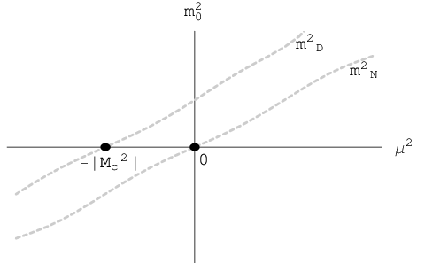
In the case of mixed BC’s on the field (i.e. relating the derivative of the field to its value at the boundaries), there is also a strict relation between the Dirichlet and the mixed BC eigenvalues .
This means that the bound for Dirichlet fields is the best one can do as far as having a negative bulk mass term. This simple general result can be seen as a generalization of the Breitenlohner-Freedman [13, 14] bound for the case of a general warped and compact 5D setup, applied to fields with either Dirichlet, Neumann or mixed BC’s:
“Instabilities will always occur in any 5D scalar field theory defined on a warped interval if it contains a negative bulk mass which is less than the critical mass required to obtain massless Dirichlet excitations. When the bulk mass is above that bound, the type of boundary conditions will affect the stability or instability of the setup”.
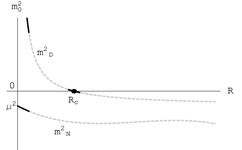
We can also look at things differently, specially perhaps if cosmological phenomenology is of interest. Instead of studying the dependence on the parameter , we can hold it fixed to some negative value and instead treat the distance between boundaries as a free parameter so that we can learn about the dependence of the eigenvalues and eigenfunctions with , while holding everything else fixed. Again, we invoke another general result from the Sturm-Liouville theory, only for the Dirichlet case this time, which states that always. This means that if we fix in such a way as to obtain a massless Dirichlet excitation, for a given boundary distance , then we know that for , we will have instabilities whereas for the system will be well behaved. Moreover, as , the lightest Dirichlet eigenvalue will always diverge to (see Figure 2). In the case of the lightest Neumann eigenvalue, we know that it must be less than the Dirichlet eigenvalue, and that when its value approaches the bulk mass (see Figure 2). The lightest eigenvalue corresponding to the mixed BC case is always below the Dirichlet one, and in this sense again, it is the Dirichlet eigenvalue which sets the tightest bound on the possible size of the interval in order to avoid instabilities when a negative bulk mass scalar is considered.
It is very illuminating to consider a simple, yet non trivial example, for which one can define explicitly both the critical mass and critical radius in a transparent way, namely a scalar field defined in a slice of .
AdS5 CASE
The background spacetime metric now contains the warp factor , where the curvature depends on the bulk cosmological constant, adequately tuned with brane tensions on the two boundaries of the interval22 2 We assume that some mechanism (for e.g. [16]) fixes and stabilizes the extra dimension, with negligible backreaction on the metric so that remains an acceptable solution.. Equation (4) becomes here
| (5) |
Solutions of this equation are well known in terms of Bessel functions (see for example [17]) but it is simpler to study the conditions to obtain a massless excitation. When setting to equation (5) the general solution is then
| (6) |
where , and and are constants. When , the hyperbolic functions are simply replaced by the trigonometric and functions33 3 And if , the solution is , with and constants.. From the previous section we already know that for Neumann boundary conditions, the massless solution corresponds to a constant and exists only when the bulk mass is zero, i.e. .
The Dirichlet case is more interesting. When it is easy to realize that there will never exist a massless solution, i.e. the setup is always stable. On the other hand, when the Dirichlet condition picks up the trigonometric function, i.e. , meaning that a massless zero mode solution can always exist as long as the interbrane distance is such that . The condition on the (negative) bulk mass is therefore . From the previous section we know that when , at least one tachyonic excitation appears, whereas for the Dirichlet system is stable.
The critical distance , for a sufficiently negative bulk mass is given by , so that when , instabilities will always exist for any type of scalar (Dirichlet, Neumann or mixed). When is negative, this indicates that the strict bound on the interval distance does not apply since Dirichlet excitations will always be stable, but Neumann excitations will be unstable (for ), and mixed BC excitations can be either stable or unstable depending on their specific BC’s [15].
Outlook
In the context of a warped and compact extra dimension, we studied the limits on a negative bulk scalar mass term such that perturbative stability is maintained. With very simple Sturm-Liouville theory techniques, we managed to show that there will always be a negative mass bound, and pointed out that the best limit will always correspond to studying the Dirichlet BC case. We also noted that even in the RS metric, one can obtain a simple and transparent negative mass bound corresponding to the Breitenlohner-Freedman bound applied to a slice of . Namely, any 5D scalar field theory will always be unstable around the background if the scalar bulk mass violates the bound , where is the interval distance and is the curvature. It is however unclear what would be the holographic interpretation of a bulk scalar field with a negative bulk mass below the original BF bound . In the usual dictionary a bulk scalar field is interpreted as a 4D field coupled to an operator with scaling dimension . Now if , this term becomes imaginary, suggesting that boundary corrections might be needed for these fields.
One can also understand the mass bound as a bound on the size of the interval, such that for a sufficiently negative bulk mass, there will always be a critical size above which the setup will always be unstable, no matter what BC’s are verified by the fields. Our original motivation for studying this setup was the search for instabilities of a Dirichlet scalar field in a warped 5D setup, in an attempt to generalize some of the results of [18, 19]. Cosmologically, one could imagine a scenario in which the interval distance changes on a cosmological time scale decoupled from the scalar field excitations scale. Then, whenever the interval size reaches the critical size, the scalar sector of the theory will have to undergo a phase transition, either restoring the scalar potential symmetries or breaking them (note that no thermal effects are considered here since this is a zero temperature analysis). It would then become necessary to study the existence and stability of other possible static configurations of the scalar field sector (coupled now to the gravitational sector), into which the system could decay. In the case of a flat spacetime (with a decoupled gravitational sector), this was studied in [18, 19] and the case of a warped extra dimension is under current investigation [20].
Acknowledgments
I would like to thank Kaustubh Agashe, Csaba Csaki, Takemichi Okui, Mark Trodden, Diana Vaman and James Wells for discussions, and the KITP center for its hospitality while finishing this manuscript. This research was supported in part by the National Science Foundation under Grant No. NSF PHY05-51164.
Appendix
Let’s consider equation (4) written in self-adjoint form
| (7) |
where , and , with being the associated eigenvalue and being the generic warp factor of the setup. Note that both and are always positive. This equation is understood as a boundary value problem in the interval and its solutions, when satisfying appropriate boundary conditions, form a complete and orthogonal set. The boundary conditions (BC) that we will consider are Dirichlet, Neumann and Mixed (or Robin) and we will write the associated eigenvalues as , and . A well known result from Sturm-Liouville theory relates the eigenvalues of different boundary conditions associated to the same self-adjoint operator, namely
| (8) |
where is the index of the solution, which corresponds to the amount of nodes that the solution has.
It turns out that one can also study the dependence of the eigenvalues with respect to the parameters of the boundary value problem, such as or in our case. One can prove the following very general results verified by the eigenvalues of different types of BC’s:
| (9) |
where positivity of is assumed. For example, let’s first write the Raleigh-Ritz formula for the eigenvalue
| (10) |
where . We can now take the variation of the Neumann eigenvalue with respect to , holding fixed and obtain simply
| (11) |
This result must be derived with care, since the eigenfunctions depend themselves on the parameter . The other positivity results can be proved in a similar fashion and are known results of the general theory of the Sturm-Liouville problem [21].
References
- [1] V. A. Rubakov and M. E. Shaposhnikov, Phys. Lett. B 125 (1983) 136.
- [2] K. Akama, Lect. Notes Phys. 176, 267 (1982) [arXiv:hep-th/0001113].
- [3] I. Antoniadis, Phys. Lett. B 246, 377 (1990).
- [4] J. D. Lykken, Phys. Rev. D 54, 3693 (1996) [arXiv:hep-th/9603133].
- [5] N. Arkani-Hamed, S. Dimopoulos and G. R. Dvali, Phys. Lett. B 429, 263 (1998) [arXiv:hep-ph/9803315].
- [6] I. Antoniadis, N. Arkani-Hamed, S. Dimopoulos and G. R. Dvali, Phys. Lett. B 436, 257 (1998) [arXiv:hep-ph/9804398].
- [7] L. Randall and R. Sundrum, Phys. Rev. Lett. 83 (1999) 3370 [arXiv:hep-ph/9905221].
- [8] L. Randall and R. Sundrum, Phys. Rev. Lett. 83, 4690 (1999) [arXiv:hep-th/9906064].
- [9] J. Hirn and V. Sanz, Phys. Rev. Lett. 97, 121803 (2006) [arXiv:hep-ph/0606086].
- [10] A. Delgado and A. Falkowski, JHEP 0705, 097 (2007) [arXiv:hep-ph/0702234].
- [11] K. Agashe, C. Csaki, C. Grojean and M. Reece, JHEP 0712, 003 (2007) [arXiv:0704.1821 [hep-ph]].
- [12] B. Batell and T. Gherghetta, Phys. Rev. D 73, 045016 (2006) [arXiv:hep-ph/0512356].
- [13] P. Breitenlohner and D. Z. Freedman, Phys. Lett. B 115, 197 (1982).
- [14] L. Mezincescu and P. K. Townsend, Annals Phys. 160, 406 (1985).
- [15] A. Delgado and M. Redi, Phys. Lett. B 562, 127 (2003) [arXiv:hep-th/0301151].
- [16] W. D. Goldberger and M. B. Wise, Phys. Rev. Lett. 83, 4922 (1999) [arXiv:hep-ph/9907447].
- [17] T. Gherghetta and A. Pomarol, Nucl. Phys. B 586, 141 (2000) [arXiv:hep-ph/0003129].
- [18] M. Toharia and M. Trodden, Phys. Rev. Lett. 100, 041602 (2008) [arXiv:0708.4005 [hep-ph]].
- [19] M. Toharia and M. Trodden, Phys. Rev. D 77, 025029 (2008) [arXiv:0708.4008 [hep-ph]].
- [20] Work in progress in collaboration with Mark Trodden and Eric West.
- [21] See for example, A. Zettl, “Sturm-Liouville Theory”, Mathematical Surveys and Monographs, Vol. 121 (AMS 2005)