∎
filou oscillation code
Abstract
The present paper provides a description of the oscillation code filou, its main features, type of applications it can be used for, and some representative solutions. The code is actively involved in CoRoT/ESTA exercises (this volume) for the preparation for the proper interpretation of space data from the CoRoT mission. Although CoRoT/ESTA exercises have been limited to the oscillations computations for non-rotating models, the main characteristic of filou is, however, the computation of radial and non-radial oscillation frequencies in presence of rotation. In particular, filou calculates (in a perturbative approach) adiabatic oscillation frequencies corrected for the effects of rotation (up to the second order in the rotation rate) including near degeneracy effects. Furthermore, filou works with either a uniform rotation or a radial differential rotation profile (shellular rotation), feature which makes the code singular in the field.
Keywords:
methods: numerical stars: evolution stars: general stars: interiors stars: oscillations (including pulsations) stars: rotation (stars: variables:) delta Scutipacs
96.60.Ly 97.10.Cv 97.10.Kc 97.10.Sj 97.20.Ge 95.75.Pq 91.30.Ab1 Introduction
Numerous oscillation codes currently provide oscillation modes for polytropes and 1D models representative of different kind of pulsating stars. The history of the oscillation code filou is particularly associated with Scuti stars. Originally developed by F. Tran Minh and L. Léon at Observatoire de Paris-Meudon (Tran Minh & Léon, 1995, see), the code has undergone several modifications and improvements in order to correct the oscillation frequencies for the effects of rotation. In particular, the inclusion of these corrections (up to the second order including near degeneracy effects) to the oscillation code and its numerical tests was part of my PhD. work (Suárez, 2002) (hereafter S02). In that work oscillation computations were extended to the case of models including a radial differential rotation profile , i.e., a radial-dependent differential rotation (the so-called shellular rotation). This last characteristic is, by now, unique, and makes this code singular in the field.
Although filou is currently optimised for the study of the pulsational behaviour of intermediate-mass classical pulsators, namely Scuti stars and Doradus stars, the code is of universal use. It has been used, for instance, to model individual Scuti stars like the well-known Altair (Suárez et al., 2005), or 29 Cygnus (Casas et al., 2006), as well as to study Scuti stars in open clusters (Suárez et al., 2002; Fox Machado et al., 2006; Suárez et al., 2007); Moreover, it has served to model high-amplitude Scuti stars (Poretti et al., 2005) and to analyse the effect of rotation on Petersen diagrams (Suárez et al., 2006a; Suárez et al., 2007). Furthermore, it is worth highlighting the work by Suárez et al. (2006b) (from now on SGM06) which takes advantage of the code’s main feature, i.e., the computation of adiabatic oscillation in presence of shellular rotation, to analyse the effect of such type of rotation on adiabatic oscillation of moderately-fast rotating Scuti stars. Concerning Doradus stars, filou has participated, additionally to other modelling works, in one of the most recent and promising asteroseismic tool for the modelling of such stars, the Frequency Ratio Method (FRM), developed by Moya et al. (2005) and Suárez et al. (2005).
From the point of view of the numerics, filou solves full sets of ODE (Ordinary Differential Equations) in a BVP (Boundary Value Problem), using a combined Galerkine – B-splines method which enhances the numerical precision with which the oscillation frequencies are calculated. Furthermore, as explained in the following sections, it is possible to easily modify numerous numerical parameters in order to adjust the calculation optimally for the required model, which makes of filou a highly versatile code.
2 The adiabatic oscillations equations and boundary conditions
filou is mainly based on the oscillations equations and their perturbations developed in Dziembowski & Goode (1992) and Soufi et al. (1998). In S02 we describe the second-order perturbation formalism used, which includes the effects of near degeneracy and considers the presence of a radial differential rotation (shellular rotation) profile, as well as its implementation in filou.
The notation followed is similar to that used by many other oscillation codes, but adapted to the theoretical development considered. Although the code works with different calculations schemes, namely, no rotation, Cowling approximation, and rotation (uniform and differential), in the present document only the most general case is considered, i.e., the presence of shellular rotation. In such a case, oscillations are computed from the so-called pseudo-rotating models, which, as explained in S02, are constructed by modifying the stellar structure equations such as to include the spherical symmetric contribution of the centrifugal acceleration, by means of an effective gravity where and are the local gravity component and the centrifugal acceleration, respectively. The effects of the non-spherical components of the deformation of the star are included through a perturbation in the oscillation equations. For instance, the perturbation of the mean density of a pseudo-rotating model is considered of the form , where is defined in SGM06 (Eq. 15).
Furthermore, when near degeneracy is taken into account, the eigenfrequency and the eigenfunction of a near-degenerate mode are then assumed of the form:
| (1) | |||||
| (2) |
where and represent the coefficients of the linear combination between the two considered degenerate modes. Subscripts and represent whatever two rotationally coupled modes. First- and second-order corrections to the eigenfrequency in presence of near degeneracy are represented by and respectively; and are the non perturbed and first-order (see definitions and details in S02 and SGM06). The computation of individual as well as the corresponding zeroth- and first-order eigenfunctions is described in the next sections.


2.1 Oscillation frequencies of a pseudo-rotating model
In order to compute the oscillation frequencies of a pseudo-rotating model, the following dimensionless quantities are used
| (3) | |||||
| (4) |
where represents the effective gravity defined in the previous section. The quantities and , represent the eulerian perturbation of the pressure and the gravitational potential (definitions of individual terms can be found in filou and SGM06). Considering a differential rotation profile of the form:
| (5) |
where represents the rotation frequency at the stellar surface, the eigenfrequencies (zeroth order) of a pseudo-rotating model are calculated from the linearised eigenvalue system:
| (6) | |||||
which is solved by filou using the dimensionless variable and the stellar radius. In the calculation the frequency is expressed in terms of the dimensionless squared frequency
| (7) |
as well as other adiabatic quantities (see Appendix in SGM06)
| (8) | |||||
| (9) | |||||
| (10) |
As in SGD98, the following variables are also employed
| (11) | |||||
| (12) | |||||
| (13) |
where and are the stellar mass and the mass enclosed in the sphere of radius , respectively.
2.2 The boundary conditions
The system above (Eqs. 6) is solved with the appropriate boundary conditions
| (14) | |||||
| (15) |
at the centre of the star and,
| (16) | |||
| (17) | |||
| (18) |
at the stellar surface. Figure 1 illustrates the solutions for the normalised eigenfunctions , , , and , corresponding to a non-radial mixed mode () obtained from a model with a surface rotational velocity of , constructed with 2100 mesh points.
2.3 First-order perturbed eigenfunctions
When near-degeneracy effects are considered, first-order corrections to the eigenfunctions are required (see Eq. 2). Considering dimensionless variables equivalent to Eq. 3–4 with first-order perturbed quantities (, , ), and the zeroth-order solutions obtained from Eq. 6. filou calculates such first-order perturbed eigenfunctions solving the following system:
| (19) | |||||
| (20) | |||||
where and . The horizontal component of can be written as follows:
| (21) |
where represents the first-order correction of the corresponding eigenfrequency.
2.4 The first- and second-order frequency corrections
Second-order frequency corrections in presence of near degeneracy (Eq. 1) are coded in filou using the following equations (S02, SGM06)
| (22) |
in the case that is , and
| (23) |
if is . In both cases first-order near degeneracy effects are implicit, which are also calculated by filou using
| (24) |
Definitions of all terms involved are given in SGM06. The and variables contains the corrections (up to the second order) for the effect of rotation on individual eigenfrequencies obtained from Eq. 6. Such corrections are coded in filou using the Saio’s notation,
| (25) |
where and . Definitions and details can be found in (SGM06, Eqs 8-15).
3 Structure & computation schemes
filou is composed by a main program and some modules written in c, and two subroutines written in fortran (77, 95), which read input data from the equilibrium models and calculate the near degeneracy effects for the rotationally coupled modes.
Computation of radial and non-radial oscillation frequencies of a given resonant cavity (input equilibrium model) is divided into three sequential steps: first, zeroth-order oscillation frequencies (eigenvalue, ) are computed as described in Sect. 2.1; then, for each eigenfrequency, the corresponding second-order frequency corrections (without including near degeneracy effects) are calculated (see Sect. 2.4). Finally, the code selects, following certain rules (see S02 or SGM06), the rotationally coupled modes (only pairs of coupled modes are considered) and calculates their corresponding near degeneracy correcting terms (also described in Sect. 2.4).
3.1 filou inputs & outputs
filou inpunts are essentially some physical quantities (see Sect. 2.1) which are read from the equilibrium model and some initial parameters. Currently, the most updated version of the code allows the use of the following input models:
-
cesam-type models: v3.*, v4.*, v5.* and 2k
-
geneve-type models
The input parameters, which are set by the user in a text file (ascii), are read by the code when executed. The main parameters are:
-
The input equilibrium model file.
-
Type of computation. This option allows the user to force some kind of computing regime (for instance, Cowling approximation, no rotation, uniform rotation, differential rotation). As well, the user can choose the type of output files required, for instance (only the list of frequencies, include or not the corrections for the effect of rotation, near degeneracy effects, or even the eigenfunctions).
-
Frequency domain and spherical degree range.
-
Type of boundary conditions (finite/infinite , see Sect.2.1)
-
Type of node assignation (zeros of or JCD method).
The basic outputs provided by filou are the list of eigenfrequencies and eigenfunctions. However, it is possible to obtain output files containing intermediate calculation data.

4 Numerical techniques
The numerical technique followed by filou is based on the Galerkin method, together with a finite sequence of B-splines, which is characterised for its flexibility, efficiency and robustness. Although the code was conceived to solve the numerical problem of stellar non-radial oscillations, it actually provides solution to any non-linear system of functional equations, and covers several specific cases, such as the method of finite elements, Lagrangian and/or hermititian of any order, or even the Crank-Nicholson method of finite differences.
Systems 6 and 20 are solved by approximating the eigenfunctions (Eqs. 3-4) with B-Spline functions. The order of such B-Splines functions can be chosen by the user, although optimum results are obtained typically for an optimal order between 4 and 6. The coefficients for each function are computed by integration following the Galerkin method. Firstly, the code scan the user-specified frequency range to obtain a first guess for the eigenfrequencies. Then, exact eigenfrequencies are searched using either the technique of dichotomy or the Newton-Raphson method.

It is worth highlighting the numerical versatility of the code, which can be optimised for the oscillations computation of very different pulsating stars, g.e., solar-like pulsators (implying high-order modes), -mode pulsators ( Doradus stars, white dwarfs), Scuti stars, etc. This is so due to the numerous numerical parameters that can be adjusted. To name a few, the precision of the solutions (zeroth- and first-order eigenfrequencies and eigenfunctions) required, the size of the internal frequency interval in which the eigenfrequencies are searched for (this optimises the calculations in the cases of high-order and low-order frequencies), the threshold for valid solutions, etc.
4.1 Numerical tests & results
In this section we report succinctly some of the numerical tests carried out on the code for its optimisation, as well as some of the tests carried out in the framework of the ESTA exercises.
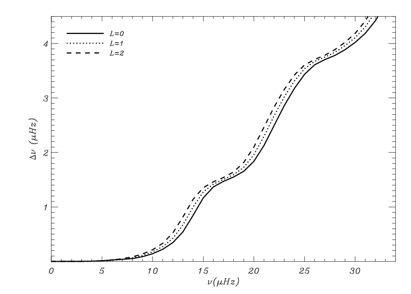
As has been shown during the ESTA exercises some of the most limiting aspects, from the numerical point of view, in the calculation of adiabatic oscillations are: the number of mesh points (including Richardson extrapolation), their distribution (rezonning), and the type of boundary conditions used. The current version of filou does not take neither Richardson extrapolation nor rezonning into account (included in the next release of the code). Nevertheless we have carried out some numerical tests of such effects, which are illustrated in Figs. 2–4, for a typical main-sequence, Scuti star model (). Notice that all the effects cause a shift in the oscillation frequency which increases as far as the radial order increases. This behaviour is exponential when varying the number of mesh points (Fig. 2) and when using Richardson extrapolation approximation (Fig. 3). In both cases, for high-order modes, the effects can reach up 10 and , respectively. For the frequency domain of Scuti stars, i.e. , such effects can reach up 1 and which are nonnegligible compared with the high-precision in frequency detection that CoRoT mission is expected to provide.


4.2 Results. The effect of shellular rotation on adiabatic oscillations
One of the most important works carried out using the oscillation code filou is the study of the effect of shellular rotation on adiabatic oscillations (SGM06). Indeed, that work takes advantage of the main feature of the code, i.e., the calculation of oscillations in presence of a radial differential rotation. Figure 5 (left panel) illustrates the effect of a shellular rotation on the radial displacement eigenfunction , for a mixed mode obtained for a , Scuti star model. Such eigenfunctions can be obtained with filou when calculating the oscillation spectra of pseudo-rotating models (see S02) computed assuming local conservation of the angular momentum. Furthermore, the effect of shellular rotation on the oscillation frequencies is also significant for Scuti stars. In Fig. 5, such an effect is depicted as a function of the radial order. In that figure and represent mode-to-mode frequency differences with (bottom panel) and without (top panel) taking the effect of near degeneracy into account. These quantities are calculated, for a given mode, as the difference between the oscillation frequency obtained assuming shellular rotation with the oscillation frequency obtained assuming uniform rotation. The term represents the additional effect of near degeneracy on the oscillation frequencies for two degenerate modes and (see SGM06 for more details). As shown in SGM06, for and mixed modes, significant effects (up to ) on the the oscillation frequencies are predicted. For high-frequency modes, such effects can reach up to . Such effects are likely to be detectable with CoRoT data, provided numerical eigenfrequencies reach the level of precision required. See SGM06 for a detailed discussion on these results.
Acknowledgements.
JCS acknowledges support at the Instituto de Astrof\́emph{i}sica de Andaluc\́emph{i}a (CSIC) by an I3P contract financed by the European Social Fund and also acknowledges support from the Spanish Plan Nacional del Espacio under project ESP2004-03855-C03-01.References
- Casas et al. (2006) Casas, R., Suárez, J. C., Moya, A., & Garrido, R. 2006, A&A, 455, 1019
- Dziembowski & Goode (1992) Dziembowski, W. A. & Goode, P. R. 1992, ApJ, 394, 670
- Fox Machado et al. (2006) Fox Machado, L., Pérez Hernández, F., Suárez, J. C., Michel, E., & Lebreton, Y. 2006, A&A, 446, 611
- Moya et al. (2005) Moya, A., Suárez, J. C., Amado, P. J., Mart\́emph{i}n-Ru\́emph{i}z, S., & Garrido, R. 2005, A&A, 432, 189
- Poretti et al. (2005) Poretti, E., Suárez, J. C., Niarchos, P. G., et al. 2005, A&A, 440, 1097
- Soufi et al. (1998) Soufi, F., Goupil, M. J., & Dziembowski, W. A. 1998, A&A, 334, 911
- Suárez (2002) Suárez, J. C. 2002, Ph.D. Thesis, ISBN 84-689-3851-3, ID 02/PA07/7178
- Suárez et al. (2005) Suárez, J. C., Bruntt, H., & Buzasi, D. 2005, A&A, 438, 633
- Suárez et al. (2002) Suárez, J.-C., Michel, E., Pérez Hernández, F., et al. 2002, A&A, 390, 523
- Suárez et al. (2007) Suárez, J.-C., Michel, E., Pérez Hernández, F., & Houdek, G. 2007, MNRAS, in press, doi 10.1111/j.1365-2966.2007.11927.x, arxiv.org/abs/0705.3626
- Suárez et al. (2006a) Suárez, J. C., Garrido, R., & Goupil, M. J. 2006a, A&A, 447, 649
- Suárez et al. (2007) Suárez, J. C., Garrido, R., & Goupil, M. J. 2007, A&A, in press
- Suárez et al. (2006b) Suárez, J. C., Goupil, M. J., & Morel, P. 2006b, A&A, 449, 673
- Suárez et al. (2005) Suárez, J. C., Moya, A., Amado, P. J., Mart\́emph{i}n-Ru\́emph{i}zw, S., & Garrido, R. 2005, A&A, 443, 271
- Tran Minh & Léon (1995) Tran Minh, F. & Léon, L. 1995, in Roxburg, I. W., Maxnou, J. L., eds., Physical Processes in Astrophysics. Lecture Notes in Physics. Springer Verlag, Berlin., 219