Coupled quantum wires

D. Makogon, N. de Jeu, and C. Morais Smith Affiliation: Institute for Theoretical Physics, University of Utrecht, Leuvenlaan 4, 3584 CE Utrecht, The Netherlands.

August 24, 2026

Abstract

We study a set of crossed 1D systems, which are coupled with each other via tunnelling at the crossings. We begin with the simplest case with no electron-electron interactions and find that besides the expected level splitting, bound states can emerge. Next, we include an external potential and electron-electron interactions, which are treated within the Hartree approximation. Then, we write down a formal general solution to the problem, giving additional details for the case of a symmetric external potential. Concentrating on the case of a single crossing, we were able to explain recent experinents on crossed metallic and semiconducting nanotubes [J. W. Janssen, S. G. Lemay, L. P. Kouwenhoven, and C. Dekker, Phys. Rev. B 65, 115423 (2002)], which showed the presence of localized states in the region of crossing.

pacs

73.21.Hb, 73.22.-f, 73.23.Hk, 73.43.Jn

I Introduction

Physics in 1D systems manifests a number of peculiar phenomena, such as spin-charge separation, conductance quantization,[1] and anomalous low-temperature behavior in the presence of backscattering impurity.[2] It is reasonable to expect that the more complex structures composed of crossed 1D systems, such as crossings and arrays, should exhibit some particular features as well. Although the transport properties of crossed 1D systems and their arrays have been thoroughly studied both theoretically[3] and experimentally[4, 5, 6], the electronic structure of these systems is much less understood and the interpretation of existing experimental results is challenging. Recent scanning tunnelling microscopy (STM) experiments on a metallic carbon nanotube crossed with a semiconducting one[7] have shown the existence of localized states at the crossing which are not due to disorder. However, these localized states do not appear systematically in all experiments, i.e. the effect is highly dependent on the nature of the carbon nanotubes (metallic or semiconducting), of the barrier formed at the crossing, etc. Aiming at clarifying this problem, we present in this paper a detailed study of tunnelling effects between crossed 1D systems in the presence of potential barriers for massive quasiparticle excitations. Because effects of electron-electron interactions can be reasonably incorporated in a random phase approximation (RPA),[8, 9] we study a simpler model, accounting for electron-electron interactions only within Hartree approximation. The outline of this paper is the following: in section II we introduce the model that we are going to use to describe the array of crossed nanowires. In section III we consider a particular case of free electrons and write down explicit solutions for the case of one and four crossings. Section IV contains formal general solution with additional details given for the case of a symmetric external potential. We demonstrate the effect of tunnelling on the electronic structure of single crossings in Section V and qualitatively discuss different possibilities depending on the external potential. Section VI contains quantitative analysis and comparison with available experimental data of the electronic structure of single crossing for different values of parameters. Our conclusions and open questions are presented in Section VII.

II The Model

We consider a system composed of two layers of crossed quantum wires with interlayer coupling. The upper layer has a set of parallel horizontal wires described by fermionic fields $\psi_{j}(x)$ , whereas the lower layer contains only vertical parallel wires described by the fields $\varphi_{i}(y)$ . The wires cross at the points $(x_{i},y_{j})$ , with $i,j\in Z$ and the distance between layers is $d$ , with $min(|x_{i}-x_{i+1}|,|y_{j}-y_{j+1}|)\gg d$ , see Fig.1.

Refer to caption — Figure 1: 2D array of crossed wires.

The partition function of the system reads

Z=\int d[\psi_{j}]d[\psi^{*}_{j}]d[\varphi_{i}]d[\varphi_{i}^{*}]e^{-S/\hbar},

(1)

with the total action given by

S=S_{0}+S_{\rm sct}+S_{\rm int}.

(2)

The first term accounts for the kinetic energy and external potential $V^{\rm ext}_{j}(x)$ , which can be different in each wire and may arise, e.g., due to a lattice deformation, when one wire is built on top of another,

	$\displaystyle S_{0}$	$\displaystyle=$	$\displaystyle\sum_{j}\int_{0}^{\hbar\beta}d\tau\int dx\psi_{j}^{*}(x,\tau)G^{-1}_{jx}\psi_{j}(x,\tau)$		(3)
		$\displaystyle+$	$\displaystyle\sum_{i}\int_{0}^{\hbar\beta}d\tau\int dy\varphi_{i}^{*}(y,\tau)G^{-1}_{iy}\varphi_{i}(y,\tau),$		(3)

where

	$\displaystyle G^{-1}_{jx}$	$\displaystyle=$	$\displaystyle\hbar\frac{\partial}{\partial\tau}-\frac{\hbar^{2}}{2m}\frac{d^{2}}{dx^{2}}+V^{\rm ext}_{j}(x)-\mu_{x},$
	$\displaystyle G^{-1}_{iy}$	$\displaystyle=$	$\displaystyle\hbar\frac{\partial}{\partial\tau}-\frac{\hbar^{2}}{2m}\frac{d^{2}}{dy^{2}}+V^{\rm ext}_{i}(y)-\mu_{y}.$		(4)

Here, $\mu_{x,y}$ denotes the chemical potential in the upper ( $\mu_{x}$ ) or lower ( $\mu_{y}$ ) layer.

The second term of Eq. (2) describes scattering at the crossings $(x_{i},y_{j})$ ,

S_{\rm sct}=\sum_{ij}\int_{0}^{\hbar\beta}d\tau H_{ij},

(5)

where

H_{ij}=\left[\psi_{j}^{*}(x_{i},\tau)\quad\varphi^{*}_{i}(y_{j},\tau)\right]\left(\begin{array}[]{cc}U_{ij}&T_{ij}\\ T^{*}_{ij}&\tilde{U}_{ij}\end{array}\right)\left[\begin{array}[]{c}\psi_{j}(x_{i},\tau)\\ \varphi_{i}(y_{j},\tau)\end{array}\right].

Notice that the matrix element $U_{ij}$ describing intra-layer contact scattering can, in principle, be different from $\tilde{U}_{ij}$ , but both must be real. On the other hand, the contact tunnelling (inter-layer) coefficient between the two crossed wires $T_{ij}$ can be a complex number, since the only constraint is that the matrix above must be Hermitian.

The third term in Eq. (2) accounts for electron-electron interactions,

	$\displaystyle S_{\rm int}$	$\displaystyle=$	$\displaystyle\frac{1}{2}\sum_{j}\int_{0}^{\hbar\beta}d\tau\int_{0}^{\hbar\beta}d\tau^{\prime}\int dx\int dx^{\prime}\psi_{j}^{}(x,\tau)\psi_{j}^{}(x^{\prime},\tau^{\prime})V^{\rm e-e}(x-x^{\prime})\psi_{j}(x,\tau)\psi_{j}(x^{\prime},\tau^{\prime})$		(6)
		$\displaystyle+$	$\displaystyle\frac{1}{2}\sum_{i}\int_{0}^{\hbar\beta}d\tau\int_{0}^{\hbar\beta}d\tau^{\prime}\int dy\int dy^{\prime}\varphi_{i}^{}(y,\tau)\varphi_{i}^{}(y^{\prime},\tau^{\prime})V^{\rm e-e}(y-y^{\prime})\varphi_{i}(y,\tau)\varphi_{i}(y^{\prime},\tau^{\prime}).$		(6)

III Free electrons case

We start by considering a very simplified case, namely, free electrons (no electron-electron interaction, $V^{\rm e-e}(x)=0$ and no external potential, $V^{\rm ext}_{j}(x)=0$ ). Moreover, we assume $\tilde{U}_{ji}=U_{ji}=0$ and put $\mu_{x}=\mu_{y}=\mu$ . The interlayer tunnelling is assumed to be equal at each crossing point $T_{ij}=T$ and to have a real and positive value. In such a case, the partition function consists of only Gaussian integrals. We can then integrate out the quantum fluctuations, which reduces the problem to just solving the equations of motion. Considering a real time evolution and performing a Fourier transformation in the time variable, we are left with the following equations of motion for the fields:

	$\displaystyle\left(-\frac{\hbar^{2}}{2m}\frac{d^{2}}{dx^{2}}-E\right)\psi_{j}(x)+T\sum_{l}\delta(x-x_{l})\varphi_{l}(y_{j})$	$\displaystyle=$	$\displaystyle 0,$
	$\displaystyle\left(-\frac{\hbar^{2}}{2m}\frac{d^{2}}{dy^{2}}-E\right)\varphi_{i}(x)+T\sum_{l}\delta(y-y_{l})\psi_{l}(x_{i})$	$\displaystyle=$	$\displaystyle 0,$		(7)

where $m$ denotes the electron mass and $E$ is the energy of an electron state. Firstly, we evaluate the solutions for the case of free electrons without tunnelling and then we investigate how the addition of tunnelling changes the results. The solution for the free electron case consists of symmetric and antisymmetric normalized modes,

\psi_{s}(x)=\frac{1}{\sqrt{L}}\cos(k_{s}x),\qquad\psi_{a}(x)=\frac{1}{\sqrt{L}}\sin(k_{a}x),

(8)

respectively. The corresponding momenta $k_{s}$ and $k_{a}$ depend on the boundary conditions: with open boundary conditions $k_{s}=\pi(2n+1)/2L$ , $k_{a}=\pi n/L$ and with periodic boundary conditions $k_{s}=k_{a}=\pi n/L$ for a wire of length $2L$ and $n$ integer. To find the solution for the case with tunnelling $T\neq 0$ , we have to solve Eqs. (7). These equations are linear, therefore, the solution consists of a homogeneous and an inhomogeneous parts,

\psi_{j}(x)=\psi_{j}^{\rm hom}(x)+\psi_{j}^{\rm inh}(x),

(9)

which are

\psi_{j}^{\rm hom}(x)=A_{j}e^{ikx}+B_{j}e^{-ikx},

(10)

\psi_{j}^{\rm inh}(x)=\frac{Tm}{\hbar^{2}k}\sum_{l}\varphi_{l}(y_{j})\sin(k|x-x_{l}|).

(11)

Imposing open boundary conditions, $\psi_{j}(\pm L)=0$ , we find

	$\displaystyle A_{j}e^{ikL}+B_{j}e^{-ikL}+\psi_{j}^{\rm inh}(L)$	$\displaystyle=$	$\displaystyle 0,$
	$\displaystyle A_{j}e^{-ikL}+B_{j}e^{ikL}+\psi_{j}^{\rm inh}(-L)$	$\displaystyle=$	$\displaystyle 0.$		(12)

Writing the above equations in a matrix notation and inverting yields

\left(\begin{array}[]{c}A_{j}\\ B_{j}\end{array}\right)=\frac{-1}{2i\sin(2kL)}\left(\begin{array}[]{cc}e^{ikL}&-e^{-ikL}\\ -e^{-ikL}&e^{ikL}\end{array}\right)\left(\begin{array}[]{c}\psi_{j}^{\rm inh}(L)\\ \psi_{j}^{\rm inh}(-L)\end{array}\right).

Substituting explicitly the expression for $\psi_{j}^{\rm inh}(\pm L)$ given by Eq. (11) and using the mathematical identity

	$\displaystyle\left(e^{ikx}\quad e^{-ikx}\right)\left(\begin{array}[]{cc}e^{ikL}&-e^{-ikL}\\ -e^{-ikL}&e^{ikL}\end{array}\right)\left(\begin{array}[]{c}\sin(kL-kx_{l})\\ \sin(kL+kx_{l})\end{array}\right)$
	$\displaystyle=\cos\left(2kL\right)\cos(kx-kx_{l})-\cos(kx+kx_{l}),$

leads, after simplifications, to the solution

	$\displaystyle\psi_{j}(x)$	$\displaystyle=$	$\displaystyle-T\sum_{l}G(x,x_{l})\varphi_{l}(y_{j}),$
	$\displaystyle\varphi_{i}(y)$	$\displaystyle=$	$\displaystyle-T\sum_{l}G(y,y_{l})\psi_{l}(x_{i}),$		(18)

where, for open boundary conditions,

	$\displaystyle G_{o}(x_{i},x_{j},E)$	$\displaystyle\equiv$	$\displaystyle\frac{m}{\hbar^{2}k\sin(2kL)}[\cos(kx_{i}+kx_{j})$		(19)
		$\displaystyle-$	$\displaystyle\cos(2kL-k\|x_{i}-x_{j}\|)],$		(19)

and the energy $E$ is related to $k$ as $E=\hbar^{2}k^{2}/2m$ . Similar calculations can be performed for the case of periodic boundary conditions, yielding Eq. (18) with

G_{p}(x_{i},x_{j},E)\equiv\frac{m}{\hbar^{2}k\sin(kL)}\cos(kL-k|x_{i}-x_{j}|).

(20)

III.1 Two crossed wires

In particular, for the simplest case of a single horizontal and a single vertical wires, with just one crossing at $(x_{0},y_{0})$ , the solution is:

	$\displaystyle\psi(x)$	$\displaystyle=$	$\displaystyle-TG(x,x_{0},E)\varphi(y_{0})$
	$\displaystyle\varphi(y)$	$\displaystyle=$	$\displaystyle-TG(y,y_{0},E)\psi(x_{0}).$		(21)

By substituting $(x,y)=(x_{0},y_{0})$ , we find that at the crossing point

	$\displaystyle\psi(x_{0})$	$\displaystyle=$	$\displaystyle-TG(x_{0},x_{0},E)\varphi(y_{0})$
	$\displaystyle\varphi(y_{0})$	$\displaystyle=$	$\displaystyle-TG(y_{0},y_{0},E)\psi(x_{0}).$		(22)

The consistency condition requires that

\left|\begin{array}[]{cc}1&TG(x_{0},x_{0},E)\\ TG(y_{0},y_{0},E)&1\end{array}\right|=0,

(23)

T^{2}G(x_{0},x_{0},E)G(y_{0},y_{0},E)=1.

(24)

The solution is even simpler if $(x_{0},y_{0})=(0,0)$ . Then, for open boundary conditions, the symmetric modes are

	$\displaystyle\psi(x)$	$\displaystyle=$	$\displaystyle\frac{\varphi(0)Tm}{\hbar^{2}k\cos(kL)}\sin(kL-k\|x\|),$
	$\displaystyle\varphi(y)$	$\displaystyle=$	$\displaystyle\frac{\psi(0)Tm}{\hbar^{2}k\cos(kL)}\sin(kL-k\|y\|),$

and the antisymmetric modes are left unchanged in comparison with Eqs. (8). Also,

G(0,0,E)=\frac{m\tan(kL)}{\hbar^{2}k},

(25)

and the secular equation (24) becomes

\left[\frac{Tm\tan(kL)}{\hbar^{2}k}\right]^{2}=1,

(26)

which splits into two transcendental equations

	$\displaystyle k^{+}$	$\displaystyle=$	$\displaystyle-\frac{Tm}{\hbar^{2}}\tan(k^{+}L),$
	$\displaystyle k^{-}$	$\displaystyle=$	$\displaystyle\frac{Tm}{\hbar^{2}}\tan(k^{-}L).$

The first one describes the shifted values of scattering states energies, whereas the second equation has an additional bound state solution with $E<0$ , if $T>T_{0}=\hbar^{2}/mL$ . The appearance of the bound state is exclusively due to the presence of tunnelling. For an electron in a wire of length $2L=10^{3}$ nm the corresponding value is $T_{0}=7.62\times 10^{-5}$ eV $\cdot$ nm and for quasiparticles the value of $T_{0}$ is typically larger, inversely proportional to their effective mass. Defining then $\kappa\equiv-ik^{-}$ and taking the thermodynamic limit $L\rightarrow\infty$ , we find $|\kappa|=Tm/\hbar^{2}$ with the corresponding bound state energy

E=-\frac{T^{2}m}{2\hbar^{2}},

(27)

and the wave function given by

\psi(x)=\frac{\sqrt{|\kappa|}}{2}e^{-|\kappa x|}.

(28)

The factor $1/2$ instead of $1/\sqrt{2}$ comes from the fact that now an electron can tunnel into the other wire, where its wavefunction $\varphi(0)=-\psi(0)$ . Eqs. (27) and (28) hold for both open and periodic boundary conditions. Since the threshold value $T_{0}$ is quite small, the bound state should exist for a typical crossing with relatively good contact. However, the energy of the state is extremely small, $E\sim 10^{-8}$ eV if $T\sim T_{0}$ . Qualitatively similar results were found by numerical computation[10, 11] of the ground-state energy of an electron trapped at the intersection of a cross formed by two quantum wires of finite width.

III.2 Four crossed wires

For the case of two wires in the upper and two in the lower layers, there are four crossings. In this case, the self consistent equations read

\left[\begin{array}[]{c}\psi_{1}(x_{1})\\ \psi_{1}(x_{2})\\ \psi_{2}(x_{1})\\ \psi_{2}(x_{2})\end{array}\right]=M(x_{1},x_{2},E)\left[\begin{array}[]{c}\varphi_{1}(y_{1})\\ \varphi_{1}(y_{2})\\ \varphi_{2}(y_{1})\\ \varphi_{2}(y_{2})\end{array}\right]

(29)

and

\left[\begin{array}[]{c}\varphi_{1}(y_{1})\\ \varphi_{1}(y_{2})\\ \varphi_{2}(y_{1})\\ \varphi_{2}(y_{2})\end{array}\right]=M(y_{1},y_{2},E)\left[\begin{array}[]{c}\psi_{1}(x_{1})\\ \psi_{1}(x_{2})\\ \psi_{2}(x_{1})\\ \psi_{2}(x_{2})\end{array}\right],

(30)

where

M(x_{1},x_{2},E)=-T\left(\begin{array}[]{cccc}G(x_{1},x_{1},E)&0&G(x_{1},x_{2},E)&0\\ G(x_{1},x_{2},E)&0&G(x_{2},x_{2},E)&0\\ 0&G(x_{1},x_{1},E)&0&G(x_{1},x_{2},E)\\ 0&G(x_{1},x_{2},E)&0&G(x_{2},x_{2},E)\end{array}\right).

(31)

The secular equation then has the form

\det[M(x_{1},x_{2},E)M(y_{1},y_{2},E)-I]=0,

(32)

which yields a rather complicated transcendental equation ( $I$ is the identity matrix). The spectral equation for bound states $E<0$ can be significantly simplified in the thermodynamic limit $L\rightarrow\infty$ . Then, with $k=i\kappa$ , for both open and periodic boundary conditions, the matrix elements become

G(x_{i},x_{j},E)=\frac{m}{\hbar^{2}|\kappa|}e^{-|\kappa(x_{i}-x_{j})|}

(33)

and the secular equation in Eq. (32) has 4 solutions with negative energy described by

$\displaystyle E$	$\displaystyle=$	$\displaystyle-\frac{T^{2}m}{2\hbar^{2}}(1-a_{1}-a_{2}+a_{1}a_{2}),$
$\displaystyle E$	$\displaystyle=$	$\displaystyle-\frac{T^{2}m}{2\hbar^{2}}(1+a_{1}-a_{2}-a_{1}a_{2}),$
$\displaystyle E$	$\displaystyle=$	$\displaystyle-\frac{T^{2}m}{2\hbar^{2}}(1-a_{1}+a_{2}-a_{1}a_{2}),$
$\displaystyle E$	$\displaystyle=$	$\displaystyle-\frac{T^{2}m}{2\hbar^{2}}(1+a_{1}+a_{2}+a_{1}a_{2}).$

Here, $a_{1}\equiv e^{-|\kappa(x_{2}-x_{1})|}$ , $a_{2}\equiv e^{-|\kappa(y_{2}-y_{1})|}$ , and $E=-\hbar^{2}\kappa^{2}/2m$ (notice the implicit dependence of $a_{1}$ and $a_{2}$ on $E$ ). The value of $a_{i}$ depends exponentially on the distance between the crossing points. In the limit $|x_{2}-x_{1}|,|y_{2}-y_{1}|\rightarrow\infty$ the value of $a_{1},a_{2}\rightarrow 0$ , which correspond to four independent crossings with the bound state energy $E=-T^{2}m/{2\hbar^{2}}$ , the same value as we found in the previous case (see Eq. (27)).

III.3 A regular lattice of crossed wires

Consider now a regular square lattice, with lattice constant $a$ . Then, one has $x_{l}=al$ and $y_{j}=aj$ . From symmetry arguments, the wave functions should be $\psi_{j}(x)=\psi_{0}(x)e^{iK_{y}aj}$ and $\varphi_{l}(y)=\varphi_{0}(y)e^{iK_{x}al}$ . After substituting them into Eq. (18) and using Eq. (33) we find

$\displaystyle\psi_{j}(x)=$	$\displaystyle-$	$\displaystyle T\varphi_{0}(y_{j})\frac{me^{iK_{x}l_{x}a}}{\hbar^{2}\kappa}\left[\frac{\sinh(\kappa x-\kappa al_{x})e^{iK_{x}a}}{\cosh(\kappa a)-\cos(K_{x}a)}\right.$
	$\displaystyle-$	$\displaystyle\left.\frac{\sinh(\kappa x-\kappa(l_{x}+1)a)}{\cosh(\kappa a)-\cos(K_{x}a)}\right],$
$\displaystyle\varphi_{l}(y)=$	$\displaystyle-$	$\displaystyle T\psi_{0}(x_{l})\frac{me^{iK_{y}l_{y}a}}{\hbar^{2}\kappa}\left[\frac{\sinh(\kappa x-\kappa al_{y})e^{iK_{y}a}}{\cosh(\kappa a)-\cos(K_{y}a)}\right.$
	$\displaystyle-$	$\displaystyle\left.\frac{\sinh(\kappa y-\kappa(l_{y}+1)a)}{\cosh(\kappa a)-\cos(K_{y}a)}\right],$

where $l_{x},l_{y}\in Z$ , such that $al_{x}\leq x<a(l_{x}+1)$ and $al_{y}\leq y<a(l_{y}+1)$ . Therefore, $\psi_{j}(x_{l})=\psi_{0}(0)e^{i(K_{x}al+K_{y}aj)}$ and $\varphi_{l}(y_{j})=\varphi_{0}(0)e^{i(K_{x}al+K_{y}aj)}$ , with $\psi_{0}(0)$ and $\varphi_{0}(0)$ related by

	$\displaystyle\psi_{0}(0)$	$\displaystyle=$	$\displaystyle-T\frac{m}{\hbar^{2}\kappa}\frac{\sinh(\kappa a)}{\cosh(\kappa a)-\cos(K_{x}a)}\;\varphi_{0}(0),$
	$\displaystyle\varphi_{0}(0)$	$\displaystyle=$	$\displaystyle-T\frac{m}{\hbar^{2}\kappa}\frac{\sinh(\kappa a)}{\cosh(\kappa a)-\cos(K_{y}a)}\;\psi_{0}(0).$		(34)

Thus, the spectral equation reads

1=\frac{(mT)^{2}}{(\hbar^{2}\kappa)^{2}}\frac{\sinh^{2}(\kappa a)}{[\cosh(\kappa a)-\cos(K_{x}a)][\cosh(\kappa a)-\cos(K_{y}a)]}.

By performing an analytic continuation $k=i\kappa$ in Eq. (34), we find an equations similar to the one obtained previously by Kazymyrenko and Douçot[12] when studying scattering states in a lattice. The spectral equation describes a band formed by bound states with energies $-T/a<E<0$ . The momenta $K_{x}$ and $K_{y}$ run in the interval $-\pi<K_{x}a,K_{y}a<\pi$ if $T\geq T_{f}=2\hbar^{2}/ma$ or inside the region $|\sin(K_{x}a/2)\sin(K_{y}a/2)|\leq T/T_{f}$ if $T<T_{f}$ . Similar results were calculated,[13] estimated,[14] and measured[15] in the context of hybridization between vertical and horizontal stripe modes in high-Tc superconductors.

IV A more general case

Now we consider a more general model, which takes into account the presence of an inhomogeneous potential $V^{\rm ext}_{j}(x)$ arising from possible lattice deformations, and includes electron-electron interactions $V^{\rm e-e}(x)$ , which will be treated at a mean field level, within the Hartree approximation $V^{\rm e-e}_{{\rm H}j}(x)$ . Each crossing $(x_{i},y_{j})$ is considered as a scattering point with tunnelling $T_{ij}$ and scattering potential $U_{ij}$ . The corresponding equations of motion then read

	$\displaystyle D_{jx}\psi_{j}(x)+\sum_{l}[U_{lj}\psi_{j}(x_{l})+T_{lj}\varphi_{l}(y_{j})]\delta(x-x_{l})$	$\displaystyle=$	$\displaystyle 0,$
	$\displaystyle D_{iy}\varphi_{i}(x)+\sum_{l}[\tilde{U}_{il}\;\varphi_{i}(y_{l})+T^{*}_{il}\psi_{l}(x_{i})]\delta(y-y_{l})$	$\displaystyle=$	$\displaystyle 0,$

where

	$\displaystyle D_{jx}$	$\displaystyle=$	$\displaystyle-\frac{\hbar^{2}}{2m}\frac{d^{2}}{dx^{2}}+V_{j}(x)-E,$
	$\displaystyle D_{iy}$	$\displaystyle=$	$\displaystyle-\frac{\hbar^{2}}{2m}\frac{d^{2}}{dy^{2}}+V_{i}(y)-E,$

with $V_{j}(x)=V^{\rm ext}_{j}(x)+V^{\rm e-e}_{{\rm H}j}(x)$ . This model is solved most easily through the Green’s function satisfying

D_{jx_{1}}G_{j}(x_{1},x_{2},E)=\delta(x_{1}-x_{2})

with

G_{j}(x_{1},x_{2},E)=G_{j}^{*}(x_{2},x_{1},E),

and the corresponding open boundary conditions,

G_{j}(x_{1},L,E)=0,\quad G_{j}(x_{1},-L,E)=0,

or the periodic ones

	$\displaystyle G_{j}(x_{1},L,E)=G_{j}(x_{1},-L,E),$
	$\displaystyle{G_{j}}^{\prime}(x_{1},L,E)={G_{j}}^{\prime}(x_{1},-L,E),$

where the prime denotes the derivative with respect to $x_{1}$ . Note that we consider real time Green’s function for a particular wire (not the whole system). The solution to the model is

	$\displaystyle\psi_{j}(x)$	$\displaystyle=$	$\displaystyle-\sum_{l}[U_{lj}\psi_{j}(x_{l})+T_{lj}\varphi_{l}(y_{j})]G_{j}(x,x_{l},E),$
	$\displaystyle\varphi_{i}(y)$	$\displaystyle=$	$\displaystyle-\sum_{l}[\tilde{U}_{il}\;\varphi_{i}(y_{l})+T^{*}_{il}\psi_{l}(x_{i})]G_{i}(y,y_{l},E),$		(35)

which we require to be normalized

\sum_{l}\left(\int|\psi_{l}(x)|^{2}dx+\int|\varphi_{l}(y)|^{2}dy\right)=1.

(36)

The self consistency condition for the value of the functions at crossing points $(x_{i},y_{j})$ yields the equations

$\displaystyle\sum_{l}[(U_{lj}G_{j}(x_{i},x_{l},E)+\delta_{il})\psi_{j}(x_{l})$
$\displaystyle+T_{lj}G_{j}(x_{i},x_{l},E)\varphi_{l}(y_{j})]$	$\displaystyle=$	$\displaystyle 0,$
$\displaystyle\sum_{l}[(\tilde{U}_{il}\;G_{s}(y_{j},y_{l},E)+\delta_{jl})\varphi_{i}(y_{l})$
$\displaystyle+T^{*}_{il}G_{i}(y_{j},y_{l},E)\psi_{j}(x_{i})]$	$\displaystyle=$	$\displaystyle 0.$	(37)

To find nontrivial solutions for the fields $\psi_{j}(x)$ and $\varphi_{i}(y)$ , the system of homogeneous equations in Eq. (37) has to be linearly dependent and hence the solution is represented by the null space of the system. This means that after writing the equations in a matrix form, the determinant of the matrix should be zero, thus leading to a spectral equation for $E$ . Moreover, bound state solutions in the thermodynamic limit $L\rightarrow\infty$ satisfy both open and periodic boundary conditions, since $\psi(\pm L)\rightarrow 0$ and $\psi^{\prime}(\pm L)\rightarrow 0$ .

To understand better the dependence of the Green’s function $G_{j}(x_{i},x_{l},E)$ on $E$ , we represent the function through the solutions of the homogenous equations,

D_{jx}\psi_{j}(x)=0.

(38)

We omit the index $j$ in what follows for simplicity. The most general and common representation, which holds for any static potential, reads as follows:

G(x_{1},x_{2},E)=\sum_{n}\frac{\psi_{\varepsilon_{n}}^{*}(x_{1})\psi_{\varepsilon_{n}}(x_{2})}{\varepsilon_{n}-E}.

(39)

Here, the function $\psi_{\varepsilon}(x)$ is the solution of the homogenous equation

\left(-\frac{\hbar^{2}}{2m}\frac{d^{2}}{dx^{2}}+V(x)-\varepsilon\right)\psi_{\varepsilon}(x)=0,

(40)

and the spectrum $\{\varepsilon_{n}\}$ is obtained by imposing the corresponding boundary conditions. Notice that in the present representation of $G(x_{1},x_{2},E)$ the functions $\psi_{\varepsilon_{n}}(x)$ have to be orthonormal. By writing $G(x_{1},x_{2},E)$ in the form given in Eq. (39), the following identity arises

\int dx^{\prime}G(x_{1},x^{\prime},E)G(x^{\prime},x_{2},E)=\frac{\partial G(x_{1},x_{2},E)}{\partial E}.

(41)

The case $x_{1}=x_{2}=0$ for free electrons is illustrated in Fig. 3, where Eq. (25) is plotted. If some external potential is present, $G(x_{0},x_{0},E)$ has the same form but the positions of the poles are shifted and the corresponding values are different.

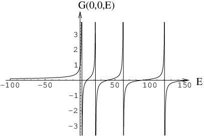
If no regularization is used, the calculations for $E>0$ must be performed in the finite size limit, otherwise with $L\rightarrow\infty$ the energy distance between different modes vanishes and the poles situated on the real positive half axis merge to form a branch cut singularity. This behavior can be readily seen on the example of Eq. (25), where can perform an analytic continuation, considering $k\rightarrow k+ik^{\prime}$ . Then, in the limit $L\rightarrow\infty$ , $\tan(kL+ik^{\prime}L)=i{\rm sgn}(k^{\prime})$ , and the function $G(x_{0},x_{0})$ changes sign as one goes from the upper to the lower complex half plane for $k\neq 0$ .

Now we represent the Green’s function through the solutions of the homogenous equation

\left(-\frac{\hbar^{2}}{2m}\frac{d^{2}}{dx^{2}}+V(x)-E\right)\psi(x)=0.

(42)

This is a second order differential equation, therefore, it should have two linearly independent solutions, which we call $\psi_{1}(x)$ and $\psi_{2}(x)$ . Then the Green’s function is

G(x_{1},x_{2},E)=\left\{\begin{array}[]{c}A_{-}\psi_{1}(x_{1})+B_{-}\psi_{2}(x_{1}),x_{1}\leq x_{2}\\ A_{+}\psi_{1}(x_{1})+B_{+}\psi_{2}(x_{1}),x_{1}>x_{2}\end{array}\right.,

(43)

where the expressions for the coefficients $A_{-},B_{-},A_{+},B_{+}$ (functions of $x_{2}$ ), are derived in the Appendix A. In particular, for a symmetric potential $V(x)$ , we can choose a symmetric $\psi_{s}(x)$ and an antisymmetric $\psi_{a}(x)$ solutions as linearly independent, i.e., $\psi_{1}(x)=\psi_{s}(x)$ and $\psi_{2}(x)=\psi_{a}(x)$ . Thus we find

G(x,0,E)=\frac{m\psi_{a}(L)}{\hbar^{2}{\psi_{a}}^{\prime}(0)}\left[\frac{\psi_{s}(x)}{\psi_{s}(L)}-\frac{\psi_{a}(|x|)}{\psi_{a}(L)}\right]

(44)

and

G(0,0,E)=\frac{m\psi_{s}(0)}{\hbar^{2}{\psi_{a}}^{\prime}(0)}\frac{\psi_{a}(L)}{\psi_{s}(L)}.

(45)

To obtain the results in the thermodynamic limit $L\rightarrow\infty$ , it is useful to rewrite $G(x_{1},x_{2})$ using quantities which do not depend on $L$ explicitly. For example,

G(x,0,E)=G(0,0,E)\frac{\psi_{s}(x)}{\psi_{s}(0)}-\frac{m}{\hbar^{2}}\frac{\psi_{a}(|x|)}{{\psi_{a}}^{\prime}(0)}.

(46)

After substitution of Eqs. (8) into Eq. (43) and simplification, for the case of noninteracting electrons we find

	$\displaystyle G(x_{1},x_{2},E)$	$\displaystyle=$	$\displaystyle\frac{m}{\hbar^{2}k\sin(2kL)}[\cos(kx_{1}+kx_{2})$
		$\displaystyle-$	$\displaystyle\cos(2kL-k\|x_{1}-x_{2}\|)],$

which is the same expression as in the previous section (see Eq. (19)). This is a posteriori justification of the use of the same letter $G(x_{1},x_{2},E)$ in the first section. The case of a harmonic potential is considered in Appendix B.

V a single crossing

Now we apply our results including tunnelling and external potential to the simpler case of only two crossed wires, aiming to compare our findings with experiments. Using the general solution given by Eq. (35), and considering $T=T^{*}$ , we can write

	$\displaystyle\psi(x)$	$\displaystyle=$	$\displaystyle-[U\psi(x_{0})+T\varphi(y_{0})]G_{1}(x,x_{0},E),$
	$\displaystyle\varphi(y)$	$\displaystyle=$	$\displaystyle-[\tilde{U}\;\varphi(y_{0})+T\psi(x_{0})]G_{2}(y,y_{0},E).$

By substituting $(x,y)=(x_{0},y_{0})$ , we find that at the crossing point

	$\displaystyle[1+UG_{1}(x_{0},x_{0},E)]\psi(x_{0})+TG_{1}(x_{0},x_{0},E)\varphi(y_{0})$	$\displaystyle=$	$\displaystyle 0,$
	$\displaystyle[1+\tilde{U}G_{2}(y_{0},y_{0},E)]\varphi(y_{0})+TG_{2}(y_{0},y_{0},E)\psi(x_{0})$	$\displaystyle=$	$\displaystyle 0.$

The consistency condition requires that

\left|\begin{array}[]{cc}1+UG_{1}(x_{0},x_{0},E)&TG_{1}(x_{0},x_{0},E)\\ TG_{2}(y_{0},y_{0},E)&1+\tilde{U}G_{2}(y_{0},y_{0},E)\end{array}\right|=0,

(47)

	$\displaystyle 0$	$\displaystyle=$	$\displaystyle[1+UG_{1}(x_{0},x_{0},E)][1+\tilde{U}G_{2}(y_{0},y_{0},E)]$
		$\displaystyle-$	$\displaystyle T^{2}G_{1}(x_{0},x_{0},E)G_{2}(y_{0},y_{0},E).$

The meaning of this equation becomes clearer in the symmetric case, when $U=\tilde{U}$ and $G_{1}(x_{0},x_{0},E)=G_{2}(y_{0},y_{0},E)=G$ . In this case, it reduces to a quadratic equation, which bears two solutions,

G_{+}=\frac{-1}{U+T},\qquad G_{-}=\frac{-1}{U-T}.

Notice that they differ by the sign in front of the tunnelling amplitude $T$ , which is shifting the potential $U$ . Such symmetry effectively reduces the problem to 1D with effective potential $U_{\rm eff}\delta(x_{0})$ . Hence, we have

	$\displaystyle\psi(x_{0})$	$\displaystyle=$	$\displaystyle\varphi(y_{0}),\quad\;\;U_{\rm eff}^{+}=U+T,$
	$\displaystyle\psi(x_{0})$	$\displaystyle=$	$\displaystyle-\varphi(y_{0}),\quad U_{\rm eff}^{-}=U-T.$		(48)

The shift of the energy levels in a wire due to the presence of the $\delta$ potential can be visualized with the help of the Green’s function expansion, where one has

G(x_{0},x_{0},E)=\sum_{n}\frac{|\psi_{\varepsilon_{n}}(x_{0})|^{2}}{\varepsilon_{n}-E}=\frac{-1}{U_{\rm eff}}.

(49)

In the case with $U_{\rm eff}=0$ , the energies are exactly those of the poles and, therefore, remain unshifted. However, since $G(x_{0},x_{0},E)=-1/U_{\rm eff}$ , the curve actually describes how the energies of the modes change as we keep increasing $-1/U_{\rm eff}$ from $-\infty$ if $U_{\rm eff}>0$ or decreasing $-1/U_{\rm eff}$ from $+\infty$ if $U_{\rm eff}<0$ . In the latter case, we can run into the region with $E<0$ , which would correspond to the appearance of a bound state. Nevertheless, to obtain an exact solution, it is more convenient to work with the expression for $G(x_{0},x_{0},E)$ in terms of the wave functions,

G(0,0,E)=\frac{m\psi_{s}(0)}{\hbar^{2}{\psi_{a}}^{\prime}(0)}\frac{\psi_{a}(L)}{\psi_{s}(L)}=\frac{-1}{U_{\rm eff}},

(50)

where we assumed $x_{0}=0$ for simplicity.

VI comparison with experiments

Now, we will compare our theoretical findings with experimental results. We concentrate mostly on the analysis of a system consisting of two crossed single wall carbon nanotubes (SWNTs): a metallic on top of a semiconducting (MS) one.[7] In its unperturbed state, the band structure of a SWNT can be understood by considering the electronic structure of graphene. Due to its cylindrical shape, the transverse momentum of one particle excitations in a SWNT has to be quantized, whereas the longitudinal momentum may vary continuously. Combining this condition with the assumption that the electronic structure is not very different from that of graphene, one finds two different situations, depending on the topology of the SWNT: there are no gapless modes and the nanotube is semiconducting, or two gapless modes are present and the nanotube is called metallic. Analyzing the spectroscopic measurements performed along the metallic nanotube (see Fig. 4) and comparing with the unperturbed electronic structure, one notices two main changes. First, a small quasi gap opens around the Fermi energy level $\varepsilon_{F}$ between $\varepsilon_{F}-0.2$ eV and $\varepsilon_{F}+0.3$ eV in the spectrum of the massless modes (corresponding to zero transverse momentum). Second, two peaks are visible at $\varepsilon_{0}=\varepsilon_{F}-0.3$ eV and $\varepsilon_{1}=\varepsilon_{F}-0.6$ eV in the region around the crossing, corresponding to localized states between the Fermi energy and the van Hove singularity at $\varepsilon_{\rm vH}=\varepsilon_{F}-0.8$ eV. Such states are not visible above the Fermi energy, thus suggesting that the electron-hole symmetry is broken by the presence of some external potential. The latter may appear due to lattice distortions and the formation of a Schottky barrier at the contact between the nanotubes. [16, 17] In the following, we show that if the potential is strong enough, localized states can form in the spectrum of the massive mode corresponding to the van Hove singularity with energy $\varepsilon=\varepsilon_{\rm vH}-E$ . Therefore, the observed localized states should have $E_{0}=-0.5$ eV and $E_{1}=-0.2$ eV.

To incorporate in a more complete way the effects of the Schottky barrier and lattice deformation, we assume $V^{\rm ext}(x)$ to have a Lorentzian shape,

V^{\rm ext}(x)=-\frac{\tilde{V}}{1+x^{2}/b^{2}}.

(51)

Firstly, we study the influence of this potential alone on the electronic structure, i.e. we assume that there is no tunnelling $T=0$ , and no electron-electron interactions. Exact numerical solution of the Schrodinger equation shows that an approximation of the potential in Eq. (51) by the harmonic one does not change the solution qualitatively. Therefore, we consider $V^{\rm ext}(x)\approx-\tilde{V}(1-x^{2}/b^{2})$ , which describes a harmonic oscillator with frequency $\omega=\sqrt{2\tilde{V}/mb^{2}}$ and corresponding spectra $E_{n}=-\tilde{V}+(n+1/2)\sqrt{2\hbar^{2}\tilde{V}/mb^{2}}$ for $E_{n}<0$ . Moreover, it is reasonable to assume that the strength of the barrier $\tilde{V}$ is of the same order as the energy of the bound states and that the potential is localized on the same length scale as the localized states. Hence, we take $\tilde{V}=0.7$ eV and $b=4$ nm. It follows then from our calculations that the difference between neighboring energy levels is quite small and there are many bound states present in the case when $m$ is the actual electron mass. However, assuming $m$ to be an effective electron mass, with $m=0.025\;m_{e}$ , which is of the same order as the experimentally estimated values $m=0.037\;m_{e}$ [18] and $m=0.06\;m_{e}$ ,[19] we find exactly two pronounced bound states: the first one has $E=-0.5$ eV and is described by the symmetric wavefunction $\psi_{s}(x)$ as shown in Fig. 5,

whereas the other has $E=-0.2$ eV and is described by the antisymmetric wavefunction $\psi_{a}(x)$ , see Fig. 6.

Considering Fig. 5, we observe that the localization size of the state is around $10$ nm, which agrees well with the experimental data. On the other hand, the state shown in Fig. 6 has a zero value exactly at the crossing and is rather spread, a behavior which is not observed experimentally. Besides these two, a number of other states are also present in the vicinity of the van Hove singularity with $E>-0.1$ eV.

Secondly, we take into account electron-electron interactions to consider other possibilities to obtain two pronounced bound states. Unfortunately, our approach only allows us to incorporate electron-electron interactions at the mean-field level by using the Hartree selfconsistent approximation

V^{\rm e-e}_{H}(x)=\int dx^{\prime}V^{\rm e-e}(x-x^{\prime})n(x^{\prime}),

(52)

where $n(x)$ is the electron density, given by

n(x)=\sum_{k}|\psi_{k}(x)|^{2}n_{F}(\varepsilon_{k}-\mu).

(53)

Here the summation $k$ goes over energy levels and $n_{F}(\varepsilon)$ is the Fermi distribution. Although it is known that in 1D systems quantum fluctuations play an extremely important role, we nevertheless start with the mean-field approximation as a first step to incorporate them in RPA. Moreover, we believe that their presence does not qualitatively change the obtained results. To render the numerical calculation simpler, we consider a delta-like interaction potential, which leads to

V^{\rm e-e}_{H}(x)=V_{0}n(x),

(54)

By estimating the effective interaction strength $V_{0}\sim 2\pi\hbar v_{F}$ from the Luttinger liquid theory, we obtain that $V_{0}\sim 3.4$ eV $\cdot$ nm for $v_{F}=8.2\times 10^{7}$ cm/s.[20] Suppose that the lowest energy state with $E=-0.5$ eV is occupied by an electron with a certain spin. Then, there is a possibility to add to the same state an electron with an opposite spin. However, due to the repulsive Coulomb interaction the energy of the two-electron state becomes $E=-0.2$ eV for $V_{0}=3.15$ eV $\cdot$ nm. The corresponding self consistent solution is presented in Fig. 7.

The state has the same shape as in Fig. 5, but is a bit more spread. By comparing the density of states (DOS) distribution with scanning tunnelling spectroscopy (STS) data for the crossing,[7] we observe that the inclusion of electron-electron interactions (Fig. 7) provides a much better agreement between theory and experiment for the $E=-0.2$ eV bound state than in the previous case (Fig. 6).

Thirdly, we take into account tunnelling between the wires. Qualitatively, this leads to the splitting of energy levels and redistribution of charge density in the wires, thus effectively reducing the strength of electron-electron interactions. Since we have no information about the electronic structure of the semiconducting nanotube, to make a quantitative estimation we assume that the effective mass is equal in both wires and that the potential is also the same. In such a case, from symmetry arguments the electron density should be evenly distributed in both wires even for a very weak tunnelling. Therefore, the electron-electron interactions should be twice stronger than in the case without tunnelling, namely, $V_{0}=6.3$ eV $\cdot$ nm to achieve the same energy value. Moreover, if the tunnelling coefficient is large enough, the splitting of the energy levels becomes significant and detectable. We can estimate the coefficient $T$ , if we assume that it has the same order for SM, metallic-metallic (MM), and semiconducting-semiconducting (SS) nanotube junctions. The SS and MM junctions have Ohmic voltage-current dependance, characterized by the conductance $G$ . Moreover, we can estimate the transmission coefficient of the junction as $G/G_{0}\sim(T/2\pi\hbar v_{F})^{2}$ , for $G/G_{0}\ll 1$ . For MM junctions experimental measurements[13] typically yield $G/G_{0}\sim 10^{-2}$ , thus corresponding to $T\sim 0.34$ eV $\cdot$ nm. For example, for $T=0.28$ eV $\cdot$ nm and $\tilde{V}=0.44$ eV in Eq. (51), without electron-electron interactions we find that the system has two bound states. The lowest energy bound state with $E=-0.5$ eV is shown in Fig. 8.

Compared with Fig. 5, the state has a peak exactly at the crossing, corresponding to a local increase of the DOS. The other bound state with $E=-0.2$ eV is shown in Fig. 9.

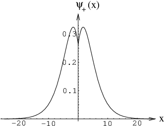
Contrary to the previous case, the state has a deep at the crossing, corresponding to a local decrease of the DOS. However, these local change in DOS is too small to be observable in the present experimental data. If we now include electron-electron interactions with $V_{0}=3.15$ eV $\cdot$ nm and add a second electron with different spin to the system, we find that the new state has $E=-0.267$ eV and acquires the shape shown in Fig. 10.

The last result suggests that there are yet other possible interpretations of the experimental results. Firstly, if the potential in the metallic SWNT is significantly decreased due to screening effects but a Schottky barrier in the semiconducting SWNT can reach considerable values, sufficient for the formation of the bound states, then the latter are also going to be present in the metallic SWNT due to tunnelling between SWNTs. Secondly, there is still a possibility to find a bound state existing purely due to tunnelling, i.e., without external potential, as was shown in Eq. (28), and a second bound state may arise with different energy due to Coulumb repulsion between electrons with different spins. However, this is most probably not the case we have in the experiments, because due to electron-hole symmetry such states would exist also above the Fermi energy, a result which is not observed experimentally.

VII Conclusions

We presented several possibilities to explain the observed localized states at the crossing of metallic and semiconducting nanotubes.[7] All of them require the existence of an external potential in the metallic and/or semiconducting SWNT to break the electron-hole symmetry, since the localized states were seen only below the Fermi energy. Most probably, such a potential comes from a Schottky barrier and the effect of lattice distortions is minimal, since such localized states were, up to now, observed only for MS crossings and not for MM or SS ones. Moreover, the effective mass of quasiparticle excitations should be of order $m=0.025\;m_{e}$ , where $m_{e}$ is the actual electron mass, to generate only a few bound states localized on a region of approximately $10$ nm with energy of order of $0.5$ eV. The best agreement with the experimental data is obtained by assuming that the second bound state has a different energy due to the Coulumb repulsion between electrons with different spins. The role of tunnelling in the observed electronic structure is not clear and allows for many interpretations. To avoid such ambiguity, the electronic structure of the semiconducting nanotube should be measured as well. Moreover, to be sure that the available STS measurements indeed represent the electronic structure of the nanotube and are free of artifacts introduced by the STM tip [21] several measurements with different tip height should be performed.

VIII ACKNOWLEDGMENTS

We are very grateful to S. G. Lemay for useful discussions.

Appendix A

Here we consider the Green’s function as a function of one variable $x_{1}$ and fix $x_{2}$ for a moment. Since $G(x_{1},x_{2},E)$ is the Green’s function, we require it to satisfy proper boundary conditions $G(\pm L,x_{2},E)=0$ , be continuous $G(x_{2}-0,x_{2},E)=G(x_{2}+0,x_{2},E)$ , and also $G^{\prime}(x_{2}-0,x_{2},E)-G^{\prime}(x_{2}+0,x_{2},E)=2m/\hbar^{2}$ . Substituting Eq. (43) into the above requirements one finds

P\left(\begin{array}[]{c}A_{+}\\ A_{-}\\ B_{+}\\ B_{-}\end{array}\right)=\frac{2m}{\hbar^{2}}\left(\begin{array}[]{c}0\\ 0\\ 0\\ 1\end{array}\right),

(55)

where

P\equiv\left(\begin{array}[]{cccc}\psi_{1}(L)&0&\psi_{2}(L)&0\\ 0&\psi_{1}(-L)&0&\psi_{2}(-L)\\ \psi_{1}(x_{2})&-\psi_{1}(x_{2})&\psi_{2}(x_{2})&-\psi_{2}(x_{2})\\ -\psi_{1}^{\prime}(x_{2})&\psi_{1}^{\prime}(x_{2})&-\psi_{2}^{\prime}(x_{2})&\psi_{2}^{\prime}(x_{2})\end{array}\right).

(56)

Multiplying the Eq. (55) by the matrix $P^{-1}$ we find

\left(\begin{array}[]{c}A_{+}\\ A_{-}\\ B_{+}\\ B_{-}\end{array}\right)=C\left(\begin{array}[]{c}\psi_{2}(L)[\psi_{2}(-L)\psi_{1}(x_{2})-\psi_{1}(-L)\psi_{2}(x_{2})]\\ \psi_{2}(-L)[\psi_{2}(L)\psi_{1}(x_{2})-\psi_{1}(L)\psi_{2}(x_{2})]\\ -\psi_{1}(L)[\psi_{2}(-L)\psi_{1}(x_{2})-\psi_{1}(-L)\psi_{2}(x_{2})]\\ -\psi_{1}(-L)[\psi_{2}(L)\psi_{1}(x_{2})-\psi_{1}(L)\psi_{2}(x_{2})]\end{array}\right),

where

C\equiv\frac{2m}{\hbar^{2}W_{r}}[\psi_{1}(L)\psi_{2}(-L)-\psi_{1}(-L)\psi_{2}(L)]^{-1}.

The Wronskian

W_{r}\equiv\psi_{1}(x_{2})\psi_{2}^{\prime}(x_{2})-\psi_{2}(x_{2})\psi_{1}^{\prime}(x_{2}),

is nonzero for linearly independent functions and its value does not depends on the point $x_{2}$ .

Appendix B

Suppose that Eq. (42) has a solution $\psi(x)$ which is neither symmetric nor antisymmetric. Thus, for symmetric potentials $\psi(-x)$ is also a solution and both of them are linearly independent. Furthermore, we can then compose a symmetric $\psi_{s}(x)=(\psi(x)+\psi(-x))/2$ and an antisymmetric $\psi_{a}(x)=(\psi(x)-\psi(-x))/2$ solutions. In particular, for a harmonic potential $V(x)=m\omega^{2}x^{2}/2$ , one can find such a solution

\psi(x)=e^{-\frac{m\omega x^{2}}{2\hbar}}H\left(\frac{E}{\hbar\omega}-\frac{1}{2},\sqrt{\frac{m\omega}{\hbar}}x\right),

(57)

where $H(\nu,x)$ is the Hermite polynomial for integer $\nu$ . It follows then that

\psi_{s}(0)=2^{\frac{E}{\hbar\omega}-\frac{1}{2}}\frac{\sqrt{\pi}}{\Gamma(\frac{3}{4}-\frac{E}{\hbar\omega})}

(58)

and

\psi_{a}^{\prime}(0)=-2^{\frac{E}{\hbar\omega}}\sqrt{\frac{2\pi\omega m}{\hbar}}\frac{1}{\Gamma(\frac{1}{4}-\frac{E}{\hbar\omega})}.

(59)

Moreover, in the thermodynamic limit $L\rightarrow\infty$ ,

G(0,0,E)=\frac{1}{2\hbar}\sqrt{\frac{m}{\omega\hbar}}\frac{\Gamma(\frac{1}{4}-\frac{E}{\hbar\omega})}{\Gamma(\frac{3}{4}-\frac{E}{\hbar\omega})}.

(60)

The Eq. (60) approaches asymptotically the expression for free fermions, as $\omega\rightarrow 0$ for $E<0$ ,

G(0,0,E)\rightarrow\frac{1}{\hbar}\sqrt{\frac{-m}{2E}}.

(61)

References

[1] M. Büttiker, Y. Imry, R. Landauer, and S. Pinhas, Phys. Rev. B 31, 6207 (1985).
[2] C. L. Kane and M. P. A. Fisher, Phys. Rev. Lett. 68, 1220 (1992).
[3] A. Komnik and R. Egger, Phys. Rev. Lett. 80, 2881 (1997).
[4] B. Gao, A. Komnik, R. Egger, D. C. Glattli, and A. Bachtold, Phys. Rev. Lett. 92, 216804 (2004).
[5] M. S. Fuhrer, J. Nygard, L. Shih, M. Forero, Young-Gui Yoon, M. S. C. Mazzoni, Hyoung Joon Choi, Jisoon Ihm, Steven G. Louie, A. Zettl, and Paul L. McEuen, Science 288, 494 (2000).
[6] H. W. Ch. Postma, M. de Jonge, Zhen Yao, and C. Dekker, Phys. Rev. B 62, 10653 (2000).
[7] J. W. Janssen, S. G. Lemay, L. P. Kouwenhoven, and C. Dekker, Phys. Rev. B 65, 115423 (2002).
[8] I. E. Dzyaloshinskii and A. I. Larkin, Zh. Eksp. Toer. Fiz. 65, 411 (1973) [So. Phys. JETP 38, 202 (1974)].
[9] S. Das Sarma and E. H. Hwang, Phys. Rev. B 54, 1936 (1996).
[10] R. L. Schult, D. G. Ravenhall, and H. W. Wyld, Phys. Rev. B 39, 5476 (1989).
[11] J. P. Carini, J. T. Londergan, K. Mullen, and D. P. Murdock, Phys. Rev. B 46, 15538 (1992).
[12] K. Kazymyrenko, B. Douçot, Phys. Rev. B 71, 075110 (2005).
[13] P. H. Dickinson and S. Doniach, Phys. Rev. B 47, 11447 (1993).
[14] A. H. Castro Neto and F. Guinea, Phys. Rev. Lett. 80, 4040 (1998).
[15] X. J. Zhou, P. Bogdanov, S. A. Kellar, T. Noda, H. Eisaki, S. Uchida, Z. Hussain, and Z.X. Shen, Science 286, 268 (1999).
[16] A. Odintsov, Phys. Rev. Lett. 85, 150 (2000).
[17] A. Odintsov and Hideo Yoshioka, Phys. Rev. B 59, 10457 (1999).
[18] P. Jarillo-Herrero, S. Sapmaz, C. Dekker, L. P. Kouwenhoven, and H. S. J. van der Zant, Nature 427, 389 (2004).
[19] M. Radosavljevic, J. Appenzeller, Ph. Avouris, and J. Knoch, Appl. Phys. Lett. 84, 3693 (2004).
[20] S. G. Lemay, J. W. Janssen, M. van den Hout, M. Mooij, M. J. Bronikowski, P. A. Willis, R. E. Smalley, L. P. Kouwenhoven, and C. Dekker, Nature (London) 412, 617 (2001).
[21] B. J. LeRoy, I. Heller, V. K. Pahilwani, C. Dekker, and S. G. Lemay, Nano Lett. 7, 2937 (2007).