Electromagnetic response and pseudo-zero-mode Landau levels
of bilayer graphene in a magnetic field
Abstract
The electromagnetic response of bilayer graphene in a magnetic field is studied in comparison with that of monolayer graphene. Both types of graphene turn out to be qualitatively quite similar in dielectric and screening characteristics, especially those deriving from vacuum fluctuations, but the effect is generally much more sizable for bilayers. The presence of the zero-(energy-)mode Landau levels is a feature specific to graphene. In bilayers, unlike in monolayers, the effect of the zero-mode levels becomes visible and even dominant in density response as an externally-controllable band gap develops. It is pointed out that the splitting of nearly-degenerate pseudo-zero-mode levels at each valley, specific to bilayer graphene, is controlled by an applied inplane electric field or by an injected current. In addition, a low-energy effective gauge theory of bilayer graphene is constructed.
pacs
73.43.-f,71.10.Pm,77.22.ChI Introduction
Graphene, a monolayer of graphite, has recently been attracting great attention, both experimentally [1, 2, 3] and theoretically, [4, 5, 6, 7, 8] for its unusual electronic transport, characteristic of relativistic” charge carriers behaving like massless Dirac fermions. Graphene is naturally of interest from the viewpoint of relativistic quantum field theory, and is a special laboratory to test the particle-hole picture [9] of the quantum vacuum and, especially in a magnetic field, to study peculiar quantum phenomena [10, 11, 12, 13, 14] tied to the chiral and parity anomalies. Actually, the half-integer quantum Hall (QH) effect and the presence of the zero-energy Landau levels observed [1, 2] in graphene are a manifestation of spectral asymmetry implied by the anomaly.
The bilayer (and multilayer) of graphene is as interesting and exotic [15, 16] as the monolayer. In bilayer graphene interlayer coupling modifies the intralayer relativistic spectra to yield a quasiparticle spectrum with a parabolic energy dispersion. [15] The relativistic feature thereby disappears but the particle-hole structure still remains, leading to a ”chiral” Schroedinger Hamiltonian, which has no analog in particle physics. Bilayer graphene, like monolayers, is intrinsically a gapless semiconductor but has a notable property that the energy gap between the conduction and valence bands is controllable [17, 18, 19, 20, 21] by use of external gates or chemical doping.
Theoretical studies show that electronic transport [4, 5, 6] and screening [22] in graphene are substantially different from those in standard planar systems. The difference becomes even more prominent under a magnetic field: [23] For graphene the vacuum state is a dielectric medium with appreciable electric and magnetic susceptibilities over all range of wavelengths. Curiously the zero-energy Landau levels, though carrying normal Hall conductance per level, scarcely contribute to the dielectric effect.
The purpose of this paper is to study the electromagnetic response of bilayer graphene in a magnetic field at integer filling factor , in comparison with that of monolayer graphene. It turns out that both types of graphene are qualitatively quite similar in dielectric and screening characteristics, but the effect is much more sizable for bilayers (because of the difference in the basic cyclotron energy).
In bilayer graphene there arise two species of zero-energy levels (or zero modes), which, when an interlayer field is applied, move up or down (oppositely) at the two valleys. Remarkably, the dielectric effects due to the (pseudo) zero modes, unlike in monolayers, become visible and even grow steadily as the tunable band gap develops. It is pointed out that the splitting of nearly degenerate pseudo-zero-mode levels at each valley, specific to bilayer graphene, is controlled by an inplane electric field or by an injected current. In addition, we construct out of the response a low-energy effective gauge theory of bilayer graphene in a magnetic field and verify that the electric susceptibility of a QH system is generally expressed as a ratio of the Hall conductance to the Landau gap.
In Sec. II we briefly review the low-energy effective theory of bilayer graphene and study its Landau-level spectrum. In Sec. III we examine the electromagnetic response and screening properties of bilayer graphene. In Sec. IV we derive an effective gauge theory. In Sec. V we study the effect of an inplane field on the almost degenerate zero-mode levels at each valley and discuss its consequences. Section VI is devoted to a summary and discussion.
II Bilayer graphene
The bilayer graphene consists of two coupled hexagonal lattices of carbon atoms, arranged in Bernal stacking, with inequivalent sites denoted as in the bottom layer and in the top layer. The electron fields in the bilayer are described by four-component spinors on the four sites and, as in the case of monolayer graphene, their low-energy spectrum is governed by the electron states near the two inequivalent Fermi points and in the Brillouin zone. The intralayer coupling eV is related to the Fermi velocity in monolayer graphene, m/s, with the lattice constant nm. The interlayer coupling and are one-order of magnitude weaker than the intralayer coupling ; numerically, [24] eV and eV.
Actually the neighboring sites and form interlayer dimers via and get shifted to higher energy bands, and the low-energy sector is essentially described by two-component spinors residing on the and sites. The effective Hamiltonian is written as [15]
where coupling to electromagnetic potentials is introduced through , , and . Here refers to the valley with and while refers to the valley with and . We suppress the electron spin, which is taken care of simply via spin degeneracy .
In the first term with a linear dispersion represents direct interlayer hopping via , with characteristic velocity , while the second term with a quadratic dispersion represents hopping via the dimer state, giving .
The takes into account a possible asymmetry between the two layers, leading to a gap between the conduction and valence bands. An important feature of bilayer graphene is that such a gap is controllable [17, 18, 19] by use of external gates, with an interlayer voltage . The second term in is a layer asymmetry associated with the depleted charge on the dimer sites; we call it a kinetic asymmetry.
Let us place graphene in a strong uniform magnetic field normal to the sample plane; to this end we set . It is convenient to rescale and with the magnetic length so that . The kinetic terms thereby acquire the scale and ; numerically, meV and meV, where stands for the magnetic field in Tesla. The associated Landau-level spectra scale like and with the level index , with ratio . Therefore the term is practically negligible, compared with the term, for higher Landau levels under a strong magnetic field. With this in mind we cast the Hamiltonian in the form
with . Here stands for half of the band gap in units of , and it seems feasible [18] to achieve an interlayer-voltage change of magnitude . Note that the kinetic asymmtry is very weak, with .
Let us for the moment set a tiny parameter . It is, then, generally seen from the structure of that its eigenmodes are the same as those of and that the spectrum of is symmetric about , except for a possible spectrum or the zero-energy spectrum of . We shall call the eigenmodes of pseudo-zero-modes, or simply ”zero” modes.
Such spectra are slightly modulated by the tiny kinetic asymmetry. For it is possible to write down the eigenmodes explicitly. The ”nonzero” modes of are Landau levels of energy
| (14) |
labeled by integers , and (or ); . Here specifies the sign of the energy . The associated eigenmodes are written as
| (15) |
where and ; are the eigenfunctions for the Landau levels of the usual Hall electron.
In bilayer graphene there arise two nearly-degenerate zero-mode levels per valley and spin, with spectrum
| (16) |
and eigenfunctions and . We take, without loss of generality, and label the Landau levels associated with the valley (i.e., the sector with ) by and those associated with the valley (the sector with ) by . Note that the zero-mode spectrum is ordered according to ; see Fig. 1. An interlayer voltage thus works to shift the zero modes oppositely at the two valleys, opening a gap , while the nonzero-mode levels get shifted only slightly and remain symmetric, apart from the asymmetry.

The zero-mode levels at each valley are degenerate for and the degeneracy remains even in the presence of the linear kinetic term. This is because the zero modes persist even for ; indeed, with has two independent solutions of power series in ,
| (17) |
with normalization factors and ; is given by with replacement and in the argument of the gamma functions. These solutions have an infinite radius of convergence in . This verifies that the index of the Dirac Hamiltonian, , is two, apart from the Landau-level degeneracy,
| (18) |
The zero-mode spectrum, corrected by the asymmetry, eventually reads
| (19) |
with and , or
| (20) |
There is a common level shift of while the tiny level splitting is practically unchanged (for ). It is thus generally difficult to resolve the almost degenerate zero-mode levels; in a sense, it is the nonzero index (18) of the Hamiltonian that underlies this stability in the zero-mode degeneracy.
In connection with the index, it would be worth remarking that has no solution; a solution of infinite power series in , starting with , fails to converge for finite . Actually the limit corresponds to the case of monolayer graphene with linear dispersion. The index thus jumps from ”2” to ”-1” as one passes from finite to infinite .
The linear kinetic term affects the spectrum of the levels only to , which is still negligible in a strong magnetic field. We shall therefore set in most of our analysis below, except in Sec. V where we discuss possible resolution of the zero-mode levels.
For actual calculations it is useful to make the Landau-level structure explicit via the expansion [25, 26] . (From now on, we shall only display the sector since the sector is obtained by reversing the signs of and .) The Hamiltonian thereby is rewritten as
| (21) |
and the charge density as
| (22) |
with the coefficient matrix
| (23) | |||||
stands for the center coordinate with uncertainty . Here
| (24) |
for , and ; ; actually are the coefficient functions for the charge density of the ordinary Hall electrons.
In a similar fashion one can derive the expression for the current operator . We omit it here, and simply remark that the current has a component coming from the asymmetry as well.
III Electromagnetic Response
In this section we study the electromagnetic response of bilayer graphene. Let us first consider the polarization function ) in Fourier space,
| (25) |
where ; the sum is taken over occupied levels and unoccupied levels . In what follows we focus on the real part of in the static limit , and denote the components coming from the virtual () transitions as
| (26) |
Actually are functions of and are thus symmetric in , which implies the relation .
For conventional QH systems the polarization function vanishes for the vacuum since the charge operator trivially annihilates the vacuum . For graphene, in contrast, because of pair creation from the Dirac sea, and even the vacuum acquires nonzero polarization
| (27) |
Some care is needed in carrying out sums over an infinite number of Landau levels, which are potentially singular. For regularization we here choose, as before, [23] to truncate the spectrum to a finite interval and let in the very end. Regularization not only keeps calculations under control but also refines them: Actually, instead of Eq. (27), one may first consider, for a given level , the polarization ”per level” by summing over all levels but , and then obtain by summing over filled levels . This gives the same result as Eq. (27) owing to the antisymmetry .
Equation (27) is an expression for the sector (). For the charge operator in the sector one may replace, in Eq. (22), by
| (28) |
i.e., with the sign of reversed. One can define accordingly and write the vacuum polarization function as . Note that these components enjoy the following property
| (29) |
This implies, in particular, that the and sectors contribute equally to the vacuum polarization , and also that is the same for the charge-conjugate states with integer. (In view of this, we shall focus on the case from now on.)
In calculating the density response we suppose that the almost degenerate zero-mode levels at each valley remain practically inseparable and treat them as both occupied or empty; accordingly we set below. Let us first look into the leading long-wavelength part of , to be denoted as , which is related to the electric susceptibility . A look into the matrix elements in Eq. (23) shows that derives only from virtual transitions to the adjacent levels () and the related ones across the Dirac sea . A direct calculation then yields
| (30) | |||||
| (31) |
for , and
| (32) |
The bottom of the Dirac sea yields , which properly makes finite. This leads to the vacuum electric susceptibility (per valley and spin)
| (33) | |||||
| (34) | |||||
An alternative expression for this is obtained by summing up the virtual processes, or , which yields
| (35) | |||||
where .
Equations (30) and (32) tell us that the susceptibility carried by a positive-energy level of the same is slightly different by terms at the two valleys. Such corrections are visible only for the zero-mode levels since the two valleys are practically indistinguishable for (up to splitting). Let us suppose that the electrons fill up an integral number of Landau levels, with uniform density . We write in terms of the filling factors of the th level for and , with both valley and spin taken into account. The electric susceptibility at integer filling is then written as
| (36) |
(This is even in , and applies to the case of holes with equally well.)
It is amusing to note here that some expressions greatly simplify for a special value : The spectrum is equally spaced, for and , apart from the splitting. For the susceptibility one finds for , and . This yields
| (37) |
which rises linearly with .
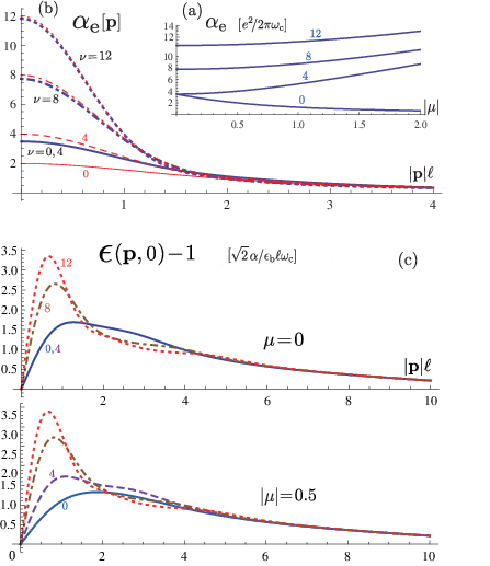
In Fig. 2 (a) we plot as a function of the band gap for and 12. The vacuum susceptibility is almost comparable to the contribution of the filled level for . The decreases gradually as the band gap develops; this is clear intuitively. In contrast, when the zero-mode levels get filled, i.e., at , starts to grow almost linearly with , and such characteristic behavior persists for higher as well. This is somewhat unexpected but is easy to understand: The zero-mode levels move linearly with the band gap while the levels are shifted only slowly, as seen from Fig. 1. The growth of is therefore due to a decrease in activation gap from the zero-mode levels. This implies that the dielectric effect due to the zero modes, though negligible for , becomes dominant for large gaps .
This is also the case with the full expression for the polarization , which one can evaluate numerically using Eqs. (23) and (26). In Fig. 2 (b) we plot the susceptibility function at 0, 4, 8, 12 for zero band gap and for a finite gap. There, as in the monolayer case, the zero-mode levels scarcely contribute to for zero gap, but one sees clearly that, as the band gap develops, they make distinct between the vacuum and the state.
The susceptibility is also related to screening properties of graphene. Let us now turn on the Coulomb interaction or with and the substrate dielectric constant , and study its effects in the random-phase approximation (RPA). The RPA dielectric function is written as [27]
| (38) |
Figure 2 (c) shows the static function for 0, 4, 8, 12, plotted in units of . Note first that there is no screening at long distances, for , as is typical of two-dimensional systems. As wave vector is increased, grows rapidly, becomes sizable for , and then decreases only gradually for larger . Such profiles of and in Fig. 2 are qualitatively quite similar to those of monolayer graphene studied earlier. [23]
Still there are some clear differences: (1) Note that the basic Landau gap of bilayer graphene, K, is about one-order of magnitude smaller than the monolayer gap K at =1T, or
| (39) |
Numerically it turns out that, for both monolayer and bilayer graphene, the vacuum susceptibility is around 3 in units of and the peak value of is around 1.8 in units of . This actually means that and are numerically more sizable for bilayers than for monolayers. In particular, for the bilayer the peak value of in Fig. 2 (c) would range from for , with the choice and 1T, or . (The value of the substrate dielectric constant depends on the structure of the sample; with SiO2 on both sides of the bilayer, e.g., one can set .) This implies that the Coulomb interaction is very efficiently screened (and weakened) in bilayer graphene.
(2) For graphene, unlike standard QH systems, even the vacuum state has an appreciable amount of polarization over a wide range of wavelengths, which reflects the quantum fluctuations or ”echoes” of the Dirac sea in response to an applied field. The echoes are in a sense ”harder” for monolayer graphene [23] for which appears almost constant over the wave-vector range in Fig. 2 (c). The rise of the peak values of with filling factor is more prominent for monolayers than bilayers; see Eq. (47). These features reflect the difference in the underlying Landau-level structures.
(3) In bilayer graphene, unlike in monolayers, the effects of the zero-mode Landau levels become visible as the band gap develops and this makes the and states distinguishable in and .
In the RPA the response function is written as , from which one can derive [28] the inter-Landau-level excitation spectra corrected by the Coulomb interaction. Isolating from one of its poles at and setting fixes the pole position of , with
| (40) |
where .
The vacuum state at supports excitons associated with the or transitions with the excitation gap and
| (41) |
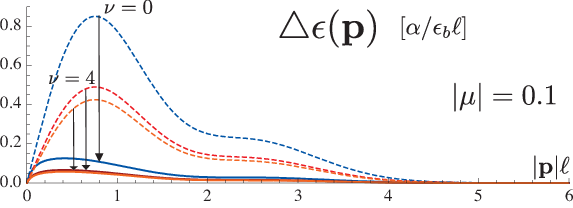
where . The state supports excitons with energy and , respectively; see Fig. 1. Similarly, at ( the transition with a gap gives rise to excitons with . As a result of screening, , one would observe prominent reduction in magnitude of the exciton spectra; see Fig. 3.
IV Effective gauge theory
In this section we study low-energy response of bilayer graphene and construct an effective gauge theory. Let us consider the Hall conductance which is read from a response of the form ; it is calculated from the current-current correlation function and from Berry’s phase as well. [14] A direct calculation similar to the one in the monolayer case [23] shows that per electron so that per filled level. The result is independent of and .
Care is needed to determine carried by the vacuum state. As before, we truncate the spectrum and find that the bottom of the Dirac sea contributes . This yields the vacuum Hall conductance
| (42) |
per valley and spin. This implies that nonzero current and charge are induced [12, 13, 14]in the vacua at the two valleys, but they combine to vanish in the vacuum, leaving no observable effect. In general, the Hall conductance is cast in the form of a spectral asymmetry and the vacuum Hall conductance is related to half of the index (18).
The long-wavelength response of bilayer graphene with uniform electron density is now summarized by the Lagrangian
| (43) | |||||
Here detects the charge density , is the electric susceptibility in Eq. (36) and stands for the magnetic susceptibility probed by a local variation about .
This response is essentially the same as that for monolayer graphene, [23] except for the values of and . Accordingly the effective theory also takes the same form, i.e., a theory of a vector field , with the Lagrangian to ,
| (44) | |||||
and the effective cyclotron frequency
| (45) |
where ; and . An advantage of bosonization [29, 30] is that it allows one to handle the Coulomb interaction exactly; it is included in Eq. (44) with shorthand notation and . (We have omitted the term from since the Coulomb interaction overtakes it at long wavelengths.)
This effective Lagrangian not only reproduces the original response (43), but also shows that the Coulomb interaction substantially modifies the dispersion of the cyclotron mode at long wavelengths ,
| (46) |
where involves , if is recovered. This excitation spectrum is in good agreement with the RPA result (40) at long wavelengths; the filling factor in Eq. (46) corresponds to in Eq. (40).
For graphene the Landau levels are not equally spaced and the excitation gaps depend on the level index or . At , e.g., the minimum gap is , and in Eq. (45) represents such an activation gap.
In particular, at where the zero-mode levels are filled, the effective gap derives solely from the vacuum fluctuations; it deviates from the true gap by about 20% for and by 5% or less for . At , and agree within 1.1% for all . The agreement is almost exact for higher . It is somewhat surprising that, as in the monolayer case, an effective theory constructed from the long-wavelength response alone gives an excellent description of the excitation spectrum. Here we verify again from Eq. (45) that the susceptibility of a QH system is generally given by a ratio of the Hall conductance to the Landau gap, [23]
| (47) |
This implies that depends on and nontrivially while it grows like for monolayer graphene.
V Zero-mode Landau levels
In this section we take a close look into the properties of the zero-mode levels at each valley, with a tiny splitting . Special care is needed in considering the response from such an almost degenerate sector, since even a weak field applied as a probe may affect the true eigenmodes. The first task therefore is to resolve the degeneracy of the sector by diagonalizing the external probe plus the asymmetry,
| (48) |
where . We suppose that is slowly varying in space and retain only terms up to first order in , i.e., . In practice, it is convenient, without loss of generality, to take , or .
We take the linear kinetic term into account (since it may potentially be important at such a low energy scale). Within the sector effectively turns [31] into the matrix Hamiltonian (in space)
| (49) |
with , ; . Here in terms of and defined in Eq. (20). Numerically,
| (50) |
The corrections are practically negligible for . We therefore set and may keep the correction to .
The Hamiltonian (49) leads to the level splitting with the new eigenmodes and related to and via the unitary transformation , with . Here we see that an inplane electric field enhances the splitting of the zero-mode levels, with a gap
| (51) |
This shows, unexpectedly, that the zero-mode level gap is controllable with an injected Hall current.
For a rough estimate let us note the following: If we take , the level gap is meV at T, with ; an applied field of strength V/cm leads to a level gap of roughly the same magnitude, as seen from
| (52) |
One can calculate the spectral weight and derive the susceptibility function associated with the transition,
| (53) |
with and spin degeneracy . (Here we have set for clarity; there is no appreciable change for .) This , with its scale set by the tiny gap , essentially governs the dielectric property of the state.
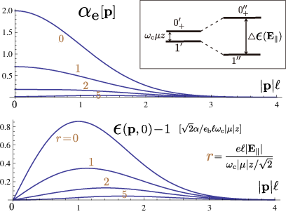
Figure 4 shows and the associated dielectric function at . It is seen that both of them decrease rapidly as becomes strong in the sequence ; this is because the and modes are chosen so as to diagonalize (for ). In Fig. 4 both and are plotted in units times as large as those in Fig. 2. Numerically, for the level gap mK at T would become as large as 300 mK ( 6.2 GHz ) by an inplane field of V/cm. This would lead to and (the peak value of in common units, i.e., one-order of magnitude larger than those in Fig. 2. This suggests that the dielectric effect would show a marked enhancement around if the level gap is resolved by an inplane field at very low temperatures.
Actually, a larger gap, which leads to better level resolution, tends to suppress the effect. Alternatively it will be more practical to observe the field-induced level gap via the QH effect with an injected current; one would be able to resolve the Hall plateaus using a suitably strong current (that may even suppress the dielectric effect). It will also be possible to detect the level gap directly by micro-wave absorption or via conductance modulations [32] associated with it.
VI Summary and discussion
In this paper we have studied the electromagnetic response of bilayer graphene in a magnetic field at integer filling factor , with emphasis on clarifying the similarities and differences in quantum features between monolayers and bilayers. Bilayer graphene has a unique feature that its band gap is externally controllable; this makes bilayers richer in electronic properties.
The particle-hole picture of the vacuum state is one of the basic features specific to graphene, both monolayers and multilayers, and is not shared with conventional QH systems. In graphene even the vacuum state responds to an external field and acts as a dielectric medium, with the Coulomb interaction being efficiently screened over the scale of the magnetic length. Graphene bilayers and monolayers are qualitatively quite similar in the vacuum dielectric characteristics (apart from some differences that reflect the underlying Landau-level structures), as we have seen in Sec. III, but numerically the dielectric effect (for the vacuum and for as well) is generally much more sizable for bilayers because of the difference in the basic Landau gap, .
The presence of the zero-energy Landau levels is another basic feature specific to graphene. The monolayer supports four zero-mode levels (one per valley and spin), while the bilayer supports eight such levels (two per valley and spin). The zero-mode levels carry normal Hall conductance per level, but in monolayers their effect is hardly visible in density response. In contrast, in bilayer graphene a gate-controlled interlayer field acts to open a band gap between the zero-mode levels at the two valleys and this valley gap, in a sense, activates them: The dielectric effect due to the pseudo-zero-mode levels grows linearly with the band gap and becomes dominant for large gaps, as we have seen in Sec. III.
A finite band gap introduces an asymmetry in the zero-mode spectrum while it leaves other levels practically symmetric. The two zero-mode levels (per spin) at each valley thereby remain degenerate, apart from a tiny kinetic splitting. This robustness in the zero-mode degeneracy at each valley as well as the presence of the zero modes itself is a consequence of the nonzero index (18) of the basic bilayer Hamiltonian (with and ). In Sec. V we have pointed out that this tiny zero-mode level gap at each valley is enhanced (and even controlled) by an inplane electric field or by an injected current. Such a gap, if properly enhanced by an injected current, may be detected via the QH effect or directly via micro-wave absorption.
Finally, in Sec. IV we have noted that the low-energy characteristics of bilayer graphene are neatly summarized by an effective Chern-Simons gauge theory, which accommodates graphene and standard QH systems equally well.
Acknowledgements.
The authors wish to thank A. Sawada for useful discussions, especially on detection of field-induced level splitting. This work was supported in part by a Grant-in-Aid for Scientific Research from the Ministry of Education, Science, Sports and Culture of Japan (Grant No. 17540253).References
- [1] K. S. Novoselov, A. K. Geim, S. V. Morozov, D. Jiang, M. I. Katsnelson, I. V. Grigorieva, S. V. Dubonos, and A. A. Firsov, Nature (London) 438, 197 (2005).
- [2] Y. Zhang, Y.-W. Tan, H. L. Stormer, and P. Kim, Nature (London) 438, 201 (2005).
- [3] Y. Zhang, Z. Jiang, J.P. Small, M.S. Purewal, Y.-W. Tan, M. Fazlollahi, J.D. Chudow, J.A. Jaszczak, H. L. Stormer, and P. Kim, Phys. Rev. Lett. 96, 136806 (2006).
- [4] Y. Zheng and T. Ando, Phys. Rev. B 65, 245420 (2002).
- [5] V. P. Gusynin and S. G. Sharapov, Phys. Rev. Lett. 95, 146801 (2005).
- [6] N. M. R. Peres, F. Guinea, and A. H. Castro Neto, Phys. Rev. B 73, 125411 (2006).
- [7] K. Nomura and A. H. MacDonald, Phys. Rev. Lett. 96, 256602 (2006).
- [8] J. Alicea and M. P. A. Fisher, Phys. Rev. B 74, 075422 (2006).
- [9] Note in this connection a proposal to simulate the Klein paradox or tunneling in graphene: M. I. Katsnelson, K. S. Novoselov, and A. K. Geim, Nat. Phys. 2, 625 (2006).
- [10] R. Jackiw and C. Rebbi, Phys. Rev. D 13, 3398 (1976); A. N. Redlich, Phys. Rev. Lett. 52, 18 (1984); R. Jackiw, Phys. Rev. D 29, 2375 (1984).
- [11] A. J. Niemi and G. W. Semenoff, Phys. Rev. Lett. 51, 2077 (1983).
- [12] G. W. Semenoff, Phys. Rev. Lett. 53, 2449 (1984).
- [13] F. D. M. Haldane, Phys. Rev. Lett. 61, 2015 (1988).
- [14] N. Fumita and K. Shizuya, Phys. Rev. D 49, 4277 (1994).
- [15] E. McCann and V. I. Fal’ko, Phys. Rev. Lett. 96, 086805 (2006).
- [16] M. Koshino and T. Ando, Phys. Rev. B 73, 245403 (2006).
- [17] T. Ohta, A. Bostwick, T. Seyller, K. Horn, and E. Rotenberg, Science 313, 951 (2006).
- [18] E. McCann, Phys. Rev. B 74, 161403(R) (2006).
- [19] E. V. Castro, K. S. Novoselov, S. V. Morozov, N.M.R. Peres, J.M.B. Lopes dos Santos, J. Nilsson, F. Guinea, A. K. Geim, and A. H. Castro Neto, Phys. Rev. Lett. 99, 216802 (2007).
- [20] H. Min, B. Sahu, S. K. Banerjee, and A. H. MacDonald, Phys. Rev. B 75, 155115 (2007).
- [21] J. B. Oostinga, H. B. Heersche, X. Liu, A. F. Morpurgo, and L. M. K. Vandersypen, Nature Materials 7, 151 (2007).
- [22] T. Ando, J. Phys. Soc, Jpn. 75, 074716 (2006); E. H. Hwang and S. Das Sarma, Phys. Rev. B 75, 205418 (2007); B. Wunsch, T. Stauber, F. Sols, and F. Guinea, New. J. Phys. 8, 318 (2006).
- [23] K. Shizuya, Phys. Rev. B 75, 245417 (2007); Phys. Rev. B 77, 075419 (2008).
- [24] L. M. Malard, J. Nilsson, D. C. Elias, J. C. Brant, F. Plentz, E. S. Alves, A. H. Castro Neto, M. A. Pimenta, Phys. Rev. B 76, 201401(R) (2007).
- [25] S. M. Girvin and T. Jach, Phys. Rev. B 29, 5617 (1984).
- [26] K. Shizuya, Phys. Rev. B 45, 11 143 (1992); Phys. Rev. B 52, 2747 (1995).
- [27] G. D. Mahan, Many-Particle Physics, (Kluwer Academic, Dordrecht/Plenum, New York, 2006).
- [28] C. Kallin and B. I. Halperin, Phys. Rev. B 30, 5655 (1984).
- [29] E. Fradkin and F. A. Schaposnik, Phys. Lett. B 338, 253 (1995).
- [30] D.-H. Lee and S.-C. Zhang, Phys. Rev. Lett. 66, 1220 (1991).
- [31] Note that the matrix element is rewritten as , with acting on ; note also that , and to .
- [32] R. S. Deacon, K.-C. Chuang, R. J. Nicholas, K. S. Novoselov, and A. K. Geim, Phys. Rev. B 76, 081406(R) (2007).