Conformal Computing: Algebraically connecting the hardware/software
boundary using a uniform approach to high-performance computation
for software and hardware applications
SPIN Springer’s internal project number, if known
Chapter \thechapter Introduction
1 General Overview
We present a systematic, algebraically based, design methodology for efficient implementation of computer programs optimized over multiple levels of the processor/memory and network hierarchy. Using a common formalism to describe the problem and the partitioning of data over processors and memory levels allows one to mathematically prove the efficiency and correctness of a given algorithm as measured in terms of a set of metrics (such as processor/network speeds, etc.). The approach allows the average programmer to achieve high-level optimizations similar to those used by compiler writers (e.g. the notion of tiling).
The approach is similar in spirit to other efforts using libraries of algorithm building blocks based on C++ template classes. In POOMA for example, expression templates using the Portable Expression Template Engine (PETE) (http://www.acl.lanl.gov.pete) were used to achieve efficient distribution of array indexing over scalar operations [1, 2, 3, 4, 5, 6, 7, 8, 9, 10].
As another example, The Matrix Template Library (MTL) [11, 12] is a system that handles dense and sparse matrices, and uses template meta-programs to generate tiled algorithms for dense matrices.
For example, the addition of two -dimensional arrays and
| (1) |
can be generalized to the situation in which multi-dimensional arrays are selected using a vector of indices .
In POOMA and were represented as classes, denoting arrays of any dimension, and expression templates were used as re-write rules to efficiently carry out the translation to scalar operations implied by:
| (2) |
The approach presented in this monograph makes use of A Mathematics of Arrays (MoA) [13] and an indexing calculus (i.e. the calculus) to enable the programmer to develop algorithms using high-level compiler-like optimizations through the ability to algebraically compose and reduce sequences of array operations.
As such, the translation from the left hand side of Eq. 2 to the right side is just one of a wide variety of operations that can be carried out using this algebra. In the MoA formalism, the array expression in Eq. 2 would be written:
| (3) |
where we have introduced the psi-operator to denote the operation of extracting an element from the multi-dimensional array using the index vector ().
In this work we demonstrate, in detail, our approach as applied to the creation of efficient implementations of the Fast Fourier Transform (FFT) optimized over multi-processor, multi-memory/network, environments. Multi-dimensional data arrays are reshaped through the process of dimension lifting to explicitly add dimensions to enable indexing blocks of data over the various levels of the hierarchy. A sequence of array operations (represented by the various operators of the algebra acting on arrays) is algebraically composed to achieve the Denotational Normal Form (DNF). The DNF is a semantic normal form expressed in terms of cartesian coordinates. Then the DNF is transformed into the ONF (Operational Normal Form) which explicitly expresses the algorithm in terms of loops and operations on indices (i.e. starts, stops, and strides are explicitly indicated). This reduction is based on an index calculus we call the -calculus. The ONF can thus be directly translated into efficient code in the language of the programmer’s choice be it for hardware or software application.
The algebra we use is a Universal Algebra based on Sylvester’s work [14] which was later embodied in the programming language APL. The algebra of MoA is a functional, enhanced subset of APL. We emphasize, however, that MoA is not a programming language but rather is a mathematical theory. Also it is important to note that APL does not have an index calculus similar to the -calculus. The notion of an index calculus was suggested by Abrams in [15] and it was extended and closed by Mullin [13].
The application we use as a first demonstration vehicle – the Fast Fourier Transform – is of significant interest in its own right. The Fast Fourier Transform (FFT) is one of the most important computational algorithms and its use is pervasive in science and engineering. This work traces the development and refinement of efficient implementations of the FFT including one in which the FFT was optimized in terms of in-cache operations leading to factors of two to four speedup in comparison with our previous records. [16] Further background material including comparisons with library routines can be found in Refs. [17, 18, 19, 20] and [16], and will be reviewed in a following section.
Our approach can be seen to be a generalization of similar work aimed at out-of-core optimizations [21]. Similarly, tensor decompositions of matrices (in general) are special cases of our reshape-transpose design. Most importantly, our designs are general for any partition size, i.e. not necessary blocked in squares, and any number of dimensions. Furthermore, our designs use linear transformations from an algebraic specification and thus they are verified. Thus, by specifying designs (such as Cormen’s and others [21]) using these techniques, these designs too could be verified.
In the context of the cache-optimized algorithm we DO NOT attempt any serious analysis of the number of cache misses incurred by the algorithm in the spirit of of Hong and Kung and others [22, 23, 24]. Rather, we present an algebraic method that achieves (or is competitive) with such optimizations mechanically. Through linear transformations we produce a normal form, the ONF, that is directly implementable in any hardware or software language and is realized in any of the processor/memory levels [25]. Most importantly, our designs are completely general in that through dimension lifting we can produce any number of levels in the processor/memory hierarchy.
One objection to our approach is that one might incur an unacceptable performance cost due to the periodic rearrangement of the data that is often needed. This will not, however, be the case if we pre-fetch data before it is needed. The necessity to pre-fetch data also exists in other similar cache-optimized schemes. Our algorithm does what the compiler community calls tiling. Since we have analyzed the loop structures, access patterns, and speeds of the processor/memory levels, pre-fetching becomes a deterministic cost function that can easily be combined with reshape-transpose or tiling operations.
Again we make no attempt to optimize the algorithm for any particular architecture. We provide a general algorithm in the form of an Operational Normal Form that allows the user to specify the blocking size at run time. This ONF therefore enables the individual user to choose the blocking size that gives the best performance for any individual machine, assuming this intentional information can be processed by a compiler11 1 Processing intentional information will be the topic of a future paper.
It is also important to note the importance of running reproducible and deterministic experiments. Such experiments are only possible when dedicated resources exist AND no interrupts or randomness effects memory/cache/communications behavior. This means that multiprocessing and time sharing must be turned off for both OS’s and Networks.
Conformal Computing22 2 The name Conformal Computing © is protected. Copyright 2003, The Research Foundation of State University of New York, University at Albany. is the name given by the authors to this algebraic approach to the construction of computer programs for array-based computations in science and engineering. The reader should not be misled by the name. Conformal in this sense is not related to Conformal Mapping or similar constructs from mathematics although it was inspired by these concepts in which certain properties are preserved under transformations. In particular, by Conformal Computing we mean a mathematical system that conforms as closely as possible to the underlying structure of the hardware. Details of the theory including discussion of MoA and -calculus are provided in the following chapter.
The bulk of the material in this monograph is devoted to the FFT. In the fourth chapter a generalized approach is presented based on the notion of a hyper-cube data structure. In the fifth chapter we extend this approach to consider and streamline certain key computational steps in a density-matrix based algorithm for simulation of quantum computers.
2 Summary of Results: Comparing with Established Library Routines
In the following sections we review previous success of the approach in which our routines were found to be competitive with, or outperformed well-established library routines. Further background can be found in Refs. [17, 18, 19, 20] and [16].
We focus on the performance of the code fragment listed in Fig.1.
do q = 1,t
L = 2**q
do row = 0,L/2-1
weight(row) = EXP((2*pi*i*row)/L)
end do
do col′ = 0,n-1,L
do row = 0,L/2-1
c = weight(row)*x(col′+row+L/2)
d = x(col′+row)
x(col′+row) = d + c
x(col′+row+L/2) = d - c
end do
end do
end do
This piece of code is the radix-2 version of a general-radix algorithm developed and tested in Ref. [19]. In the following comparisons, we refer to this routine as fftpsirad2.
3 Performance of the Radix-2 FFT
Our radix 2 experiments were run on three dedicated systems:
- 1.
a SGI/Cray Origin2000 at NCSA33 3 This work was partially supported by National Computational Science Alliance, and utilized the NCSA SGI/CRAY Origin2000 in Illinois, with 48, 195Mhz R10000 processors, and 14GB of memory. The L1 cache size is 64KB (32KB Icache and 32 KB Dcache). The Origin2000 has a 4MB L2 cache. The OS is IRIX 6.5.
- 2.
an IBM SP2 at the MAUI High Performance Computing Center44 4 We would like to thank the Maui High Performance Computing Center for access to their IBM SP2., with 32, P2SC 160Mhz processors, and 1 GB of memory. The L1 cache size is 160KB (32KB Icache and 128KB Dcache), there is no L2 cache. The OS is AIX 4.3.
- 3.
a SUN SPARCserver1000E, with 2, 60Mhz processors, and 128MB of memory. Its L1 cache size is 36KB (20KB Icache and 16KB Dcache) and it is one-way set associative. The OS is Solaris 2.7.
We tested against the FFTW on all three machines and against the math libraries supported on the IBM SP2 and the Origin 2000 machines; on the Origin 2000: IMSL Fortran Numerical Libraries version 3.01, NAG version Mark 19, and SGI’s SCSL library, and on the SP2: IBM’s ESSL library.
3.1 Experiments
Experiments on the Origin 2000 were run using bsub, SGI’s batch processing environment. Similarly, on the SP2 experiments were run using loadleveler. In both cases we used dedicated networks and processors with ALL multiprocessing and time sharing DISABLED. The SPARCserver 1000E was a machine dedicated to running our experiments. Experiments were repeated a minimum of three times and averaged for each vector size ( to ). Vendor compilers were used with the -O3 and -Inline flags, for improved optimizations (i.e. no special flags, noting the combinatorial explosion of combinations of flags one might use in an ad hoc approach). We used Perl scripts to automatically compile, run, time all experiments, and to plot our results for various problem sizes.
We believe that:
“the only consistent and reliable measure of performance is the execution time of real programs, and that all proposed alternatives to time as the metric or to real programs as the items measured have eventually led to misleading claims or even mistakes in computer design.” [26]
Therefore, we time the execution of the entire executable, which includes the creation of the FFTW plan. Although FFTW claims a plan can be reused, the plan is a data structure and not easily saved. Therefore, they have developed a utility called wisdom, which still requires partial plan regeneration.
“FFTW implements a method for saving plans to disk and restoring them. The mechanism is called wisdom. There are pitfalls to using wisdom, in that it can negate FFTW’s ability to adapt to changing hardware and other conditions. Actually, the optimal plan may change even between runs of the same binary on identical hardware, due to differences in the virtual memory environment. It is therefore wise to recreate wisdom every time an application is recompiled.” [27]
This is further confirmed by the fact that when we ran FFTW’s test program on our dedicated machines we found surprising differences in time for the same vector size. Our dedicated machines ran a default OS, e.g. no special quantum, queue settings, or kernel tuning. Due to this, a plan should be as current as possible.
IMSL, NAG, SCSL, and ESSL required no plan generation. The entire execution of code created to use each library’s FFT was timed.
3.2 Evaluation of Results
3.3 Origin 2000 Results
Performance results for our monolithic FFT code, fftpsirad2, indicate a doubling of time when the vector size is doubled for all vector sizes. IMSL doubled its performance up to . At there is an apparent memory change causing a degradation in performance. For NAG this degeneration begins at . The SGI library, SCSL, is apparently doing very machine specific optimizations, perhaps out of core techniques similar to Cormen [21] as evidenced by nearly identical performance times for and .
Against the FFTW, we achieved a performance improvement for vector sizes greater than . We ran slightly slower for the vectors through , with a maximum difference in speed of 0.013 seconds.
Both programs were able to run for the vector size (inputs of and greater, result in stack frame larger than system limit error on compile). Therefore, we achieved a large performance increase for the upper vector sizes, while our performance remained competitive for the lower sizes.
| Origin 2000 | |||||
|---|---|---|---|---|---|
| Size | fftpsirad2 | IMSL | NAG | SCSL | FFTW |
| 0.190 | 0.064 | 0.010 | 0.065 | 0.013 | |
| 0.018 | 0.061 | 0.010 | 0.047 | 0.013 | |
| 0.018 | 0.062 | 0.010 | 0.065 | 0.014 | |
| 0.017 | 0.116 | 0.011 | 0.073 | 0.013 | |
| 0.019 | 0.063 | 0.010 | 0.068 | 0.015 | |
| 0.018 | 0.062 | 0.011 | 0.105 | 0.014 | |
| 0.017 | 0.122 | 0.011 | 0.069 | 0.014 | |
| 0.021 | 0.065 | 0.013 | 0.056 | 0.015 | |
| 0.021 | 0.064 | 0.016 | 0.058 | 0.017 | |
| 0.021 | 0.067 | 0.023 | 0.067 | 0.023 | |
| 0.022 | 0.075 | 0.036 | 0.065 | 0.030 | |
| 0.024 | 0.144 | 0.065 | 0.066 | 0.051 | |
| 0.030 | 0.120 | 0.135 | 0.110 | 0.082 | |
| 0.040 | 0.209 | 0.296 | 0.080 | 0.189 | |
| 0.065 | 0.335 | 0.696 | 0.072 | 0.395 | |
| 0.126 | 0.829 | 3.205 | 0.075 | 0.774 | |
| 0.238 | 3.007 | 9.538 | 0.096 | 2.186 | |
| 0.442 | 9.673 | 18.40 | 0.143 | 4.611 | |
| 0.884 | 23.36 | 38.93 | 0.260 | 9.191 | |
| 1.910 | 46.70 | 92.75 | 0.396 | 19.19 | |
| 4.014 | 109.4 | 187.7 | 0.671 | 48.69 | |
| 7.550 | 221.1 | 442.7 | 1.396 | 99.10 | |

3.4 SP2 Results
Our routine fftpsirad2 outperforms ESSL for vector sizes up to , except for two cases. For and our performance is nearly identical. Our times continue to double from to . Comparatively, for through ESSL appears to be doing some machine specific optimizations, which subsequently double in performance through , and fail for and higher. Consequently, we perform competitively for all but five vector sizes, and we are able to process vectors up to 6,291,456 elements larger.
Against the FFTW, we achieved a performance improvement for every vector size from through , except for the single vector size . Due to our optimizations, our code, fftpsirad2, ran successfully for the vector size (inputs of and greater, result in a not enough memory available to run error at runtime). The largest size vector the FFTW was able to run on this system was . Therefore we achieved a performance increase for every size except one, and we were able to run successfully for a vector 4,194,304 elements larger.
| IBM’s SP2 | |||
|---|---|---|---|
| Size | fftpsirad2 | ESSL | FFTW |
| 0.010 | 0.013 | 0.020 | |
| 0.010 | 0.053 | 0.020 | |
| 0.010 | 0.013 | 0.020 | |
| 0.010 | 0.013 | 0.020 | |
| 0.010 | 0.013 | 0.027 | |
| 0.010 | 0.016 | 0.023 | |
| 0.010 | 0.010 | 0.020 | |
| 0.010 | 0.013 | 0.023 | |
| 0.013 | 0.010 | 0.023 | |
| 0.020 | 0.020 | 0.023 | |
| 0.033 | 0.030 | 0.030 | |
| 0.040 | 0.043 | 0.053 | |
| 0.070 | 0.060 | 0.083 | |
| 0.140 | 0.120 | 0.143 | |
| 0.280 | 0.160 | 0.283 | |
| 0.580 | 0.310 | 0.683 | |
| 1.216 | 0.610 | 1.456 | |
| 2.580 | 1.276 | 3.273 | |
| 5.553 | 3.663 | 6.770 | |
| 12.12 | Failed | 15.553 | |
| 25.25 | Failed | Failed | |

3.5 SUN SPARCserver 1000E results
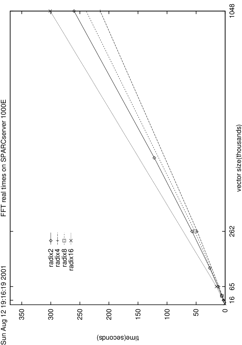
Our results on the SPARCserver 1000E, shown in Fig. 4, achieved performance improvement for every vector size except three. Additionally, we were able to run for the vector size (inputs of and greater, result in an integer overflow error on compile). The FFTW failed for , and for it ran for over 34 hours.

4 Performance of the General-Radix FFT
In this and following sections we review the performance of our general radix algorithm, developed and tested in Ref. [19].
We’ve discussed how to design and build a faster radix 2 FFT, and the results we’ve achieved. Using the same theoretical framework we can extend this design and subsequent implementations to handle any radix. Given a particular architecture and its memory hierarchy, a radix other than 2 may be more appropriate. For example, if a machine has an -way associative cache, then radix- should be used (with ), thus decreasing control time.
By generalizing the algorithm, we can investigate how a change in radix affects performance without changing the algorithm and subsequent executable. In what follows, we refer to our radix-n FFT as fftpsiradn. Fig. 5 illustrates our F90 software realization for the body of the radix 2 butterfly. Observe that the variable c is a scalar and ebase is implicitly calculated based on radix 2, i.e. 1 and -1. Also, observe that the butterfly is explicitly done using F90 syntax. In the generalized code, Fig. 6, c becomes a vector whose length is equal to the (radix - 1). Hence for radix 2, c is a one component vector, the variable base (see Fig. 6), is used to designate the radix desired.
                c = ww(j_)*z(i_+j_+L)
                z((/ i_+j_ , i_+j_+L /)) =
                   (/ z(i_+j_)+c , z(i_+j_)-c /)
          c(start) = z(i_+j_)
          ebase(start) = 1
          do k_=start+1,base-1
             c(k_) = ww(j_*k_)*z(i_+j_+(k_*L))
             z(i_+j_) = z(i_+j_)+c(k_)
             ebase(k_)=EXP((-2*pi*i)/base)**k_
          end do

          do k_=start+1,base-1
             temp = c(start)
             do l_=start+1,base-1
                temp = temp+c(l_)*
                    ebase(modulo((k_*l_),base))
             end do
             z(i_+j_+(k_*L))=temp
          end do
4.1 General Radix Issues
When a vector has length , a radix 2 FFT may be used. Whenever the same vector is a power of 4, 8, 16, etc. that radix FFT may also be used: i.e.: when = where . For example, = 64 = = = = . Hence, for a vector length 64, radix 2, 4, 8 or 64 may be used. Depending on the size of the cache, the number of cache lines, associativity of the cache, etc. one radix may perform better on one architecture over another. The reason for this is when radix 2 is used on an input vector of length n, the butterfly takes two inputs and requires iterations.
For radix 4, there are four inputs iterations, etc. Consequently, the butterfly width and the number of elements becomes the deciding factor in performance. Using one executable increases flexibility across machines.
Incidentally, the implications of an n-way n-radix FFT is that when a quantum machine is built, i.e. when all bits can interact with all bits at the same time, this algorithm will scale to that machine.
4.2 Experimental Environment
Our general radix experiments were run on two dedicated systems:
- 1.
a SUN SPARCserver1000E. This machine has two 60Mhz processors, and 128MB of memory. Its L1 cache size is 36KB (20KB Icache and 16KB Dcache) and it is one-way set associative. The OS is Solaris 2.7.
- 2.
a SUN 20. This machine has a single 50 Mhz processor, and 64 MB of memory. The OS is Solaris 2.7.
4.3 General Radix Experiments
The SPARCserver 1000E and the SUN 20 were both machines dedicated to running our experiments. We ran our experiments for a variety of different radices, given the following constraints on the input vector length: = , , , . In determining what results to discuss and represent in our graphs, we removed the following radices: 128, and 256. Their non-competitive performance results is plausibly a consequence of no machines having a cache with 128 or 256 way associativity. If this changes in the future, our executable could adapt. Table 3 illustrates performance times given a vector size 16,777,216, using an FFT radix of 2, 4, 8, 16 and 64.
4.4 Evaluation of Results
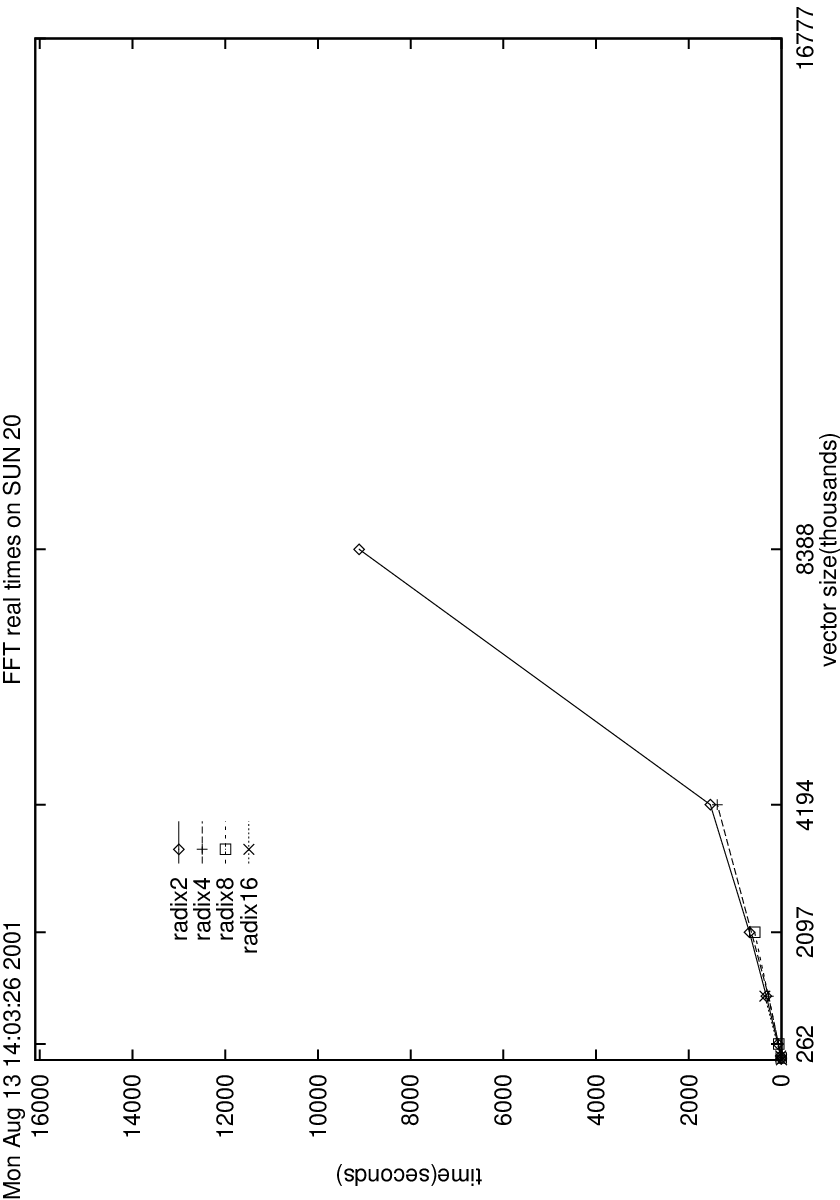
We now turn to a comparison of the general radix algorithm of various platforms as illustrated in Figs. 7, through 10.
Radix 8 performed best on the SUN 20 with a maximum vector size of 16,777,216. The performance of radix 2 and 4 experiments were impacted greatly by the number of page faults. This is, due to the fact that radix 4 performs twice as many iterations as radix 8, and radix 2 performs four times as many as radix 8. Each iteration will have about the same number of page faults as the previous, due to the fact that every sample is accessed on every iteration. The number of page faults recorded for these experiments is increased by almost these same factors.
Radix 8 has twice as many iterations as radix 16, and as expected the number of page faults is higher, but radix 8 outperforms radix 16. We conjecture that this is due to the large number of cache misses occurring at radix 16 and higher, as can be seen by an increase in user time in Table 4. The cache misses are occurring at this higher vector size because 16 samples are being processed at the same time rather than 8. Either all 16 components don’t fit in cache or many are mapping to the same cache block, hence they must wait to be loaded. Therefore, although there are fewer page faults, the higher number of cache misses are causing radices greater than or equal to 16 to incur performance degradation. Notice when comparing the SPARCserver 1000E one processor performance to the SUN 20 for vector sizes , the graphs are nearly identical. Performance also appears similar from through . Since the SUN 20’s memory was half the size of the SPARCserver 1000E’s we observe virtual behavior sooner. More memory is available on the SPARCserver 1000E even though we are using one processor.
4.5 SPARCserver 1000E’s Results (One 60 MHz Processor)

| Data | % | % | Total | ||
|---|---|---|---|---|---|
| Fault | Page | Data | User | Run | |
| Radix | Time | Faults | Time | Time | Time |
| 2 | 9318 | 779628 | 50 | 28 | 15235 |
| 4 | 5198 | 411978 | 46 | 35 | 9693 |
| 8 | 3649 | 289973 | 35 | 43 | 8381 |
| 16 | 2903 | 237271 | 26 | 52 | 8890 |
| 64 | 2582 | 195693 | 13 | 66 | 16040 |
Table 4: Paging Statistics for vector size 16,777,216 as Reported by SPARCworks, times are in Seconds
Notice the steady decrease in the number of page faults as the radix increases, this is caused by the number of iterations decreasing by a factor of two as each radix increases by a factor of two. As expected the amount of time the application spends in page faulting is directly related to the radix. Equally important is the steady increase in the percentage of user time as the radix increases, thus implying an increase in cache misses.

4.6 Conclusions for the General Radix Approach
We have succeeded in simplifying a solution to a complex problem: faster and bigger FFTs. Reproducible experiments indicate that our designs outperform all tested packages in either all, or a majority of the cases, while remaining competitive in the others.
Our single, portable, scalable executable of approximately 2,600 bytes (which can be easily built in software, hardware, or both) also must be compared with the large suite of machine–specific software required by NAG, IMSL, SCSL, ESSL, and FFTW. For example, FFTW’s necessary libraries, codelets, etc. total approximately 7,120,000 bytes.
The FFTW install is potentially complicated. It requires knowledge of makefiles, compiler options, and hand-tuning to work around variants of OSs. For example, the FFTW install fails with the default Solaris cc compiler, requiring a path change to Solaris’s SUNWspro cc compiler. The user must know that a new plan is needed for every vector size and they need to decide whether to attempt to use wisdom to save a plan.
The time and investment it takes to create a scientific library also needs to be factored into an analysis of the software. New machine designs require the reprogramming of these large libraries in order to maintain their performance. This will result in an increase of the library size as new machines are added. Also, the skill level of the scientific programmer who supports these libraries, and their knowledge of each machine is very high. The user of these machine-specific libraries must have a deep understanding of the package itself and the system on which it runs. Many of these packages require numerous parameters; fifteen for ESSL, and eight for SCSL. An incorrect decision for these parameters can result in poor performance and even possibly incorrect results. Consequently, the learning period to adapt to new software usage can be enormous from a user perspective.
In comparison, our monolithic algebraic approach to design is based on mechanizable linear transformations, which begin with a high-level specification, e.g. MATLAB, Mathematica, Maple, etc. We have found that scientists prefer these high-level languages to rapidly prototype their designs [28], as opposed to interfacing with programmers. Consequently, it is imperative that languages such as MATLAB compile to efficient code. This would necessitate such languages identifying a functional subset that embodied MoA and Psi Calculus.
Our monolithic approach addresses these issues. Our approach has no learning curve, a single executable can be used independent of vector size or machine. Additionally, a naive user of fftpsirad2 and fftpsiradn need only know the vector size on any platform. Furthermore, our monolithic algebraic approach to design is extensible to cache and other levels of the memory hierarchy, as well as parallel and distributed computing [25].
We have discovered that radix 2 is not always the best radix to choose for vectors whose length is a power of two. This opens other interesting questions: is it better to pad to radix 2 or use another radix?55 5 Padding is the usual way of handling vector lengths not equal to We believe our research into a general radix formulation may yield further optimizations for FFTs.
Our research shows a systematic way of analyzing memory access patterns and subsequent performance of the FFT on one dimensional66 6 Multi-dimensional FFTs may be built from the one dimensional FFT. arrays whose length is .
Besides determining the constituent components of the sequential FFT, e.g. bit reversal or butterfly, the radix used is of paramount importance. By developing algorithms for software, e.g., fftpsiradn, we are guaranteed that all instructions, loops and variables remain constant during the execution of the program. Hence, through monolithic analysis we can in concert, analyze the algorithm, the program, and the environment.
5 Effects Due to Specilized Hardware
In this section we review published work in which the effects due to the use of specialized hardware are illustrated [16]. Specifically we compare our routine with one that was specifically designed to exploit hardware with the capability to carry out the operation of multiply and add in one step. We find that our generic radix-2 FFT (see Fig. 1) is competitive on such hardware and is superior on a machine lacking the specialized hardware.
The study presented in Ref. [16] is a benchmark of our radix-2 FFT fftpsirad2 [19] in the context of the plane-wave based electronic structure code Abinit [29]. Such codes rely heavily on the use of the FFT and considerable work has been expended to optimize performance [30]. Therefore this context serves as a further stringent benchmark test of our routine. The purpose of this work was NOT to claim that we have the best FFT. Rather we emphasize that our approach leads to efficient code based on general principles without any hardware-specific optimization (which naturally can be included as a further refinement).
We now turn our attention to a study of the one-dimensional FFT. In comparisons between our routine, which we denote as the “CC” routine, we will refer to the Abinit routine as the “Ab” [29, 30].
We have carried out benchmark performance tests of our -dimensional FFT in comparison with the routine taken from the Abinit code [29, 30] using the same platforms as were used in previous tests: the Origin 2000 at NCSA [31] and the IBM SP2 at Maui [19, 32]. The benefit of our focus on the -dimensional transform, lies in the fact that it serves as a control test for later developments (multi-dimensional arrays and multi-level, multi-processor memories).
The following tests were carried out. We ran both routines as single processor jobs with the -O3 compiler option (f90 compiler on NCSA, and xlf on Maui) in a dedicated environment. For comparison, therefore, the -dimensional transform of Ref. [30] was run as a -dimensional transform by considering arrays of size , , and where with . Slightly better performance was obtained for the case so these are the results that we will use for comparisons with the CC routine. Perl scripts were used to compile the jobs for each size, time the execution, and collect the results. The timings from the runs involving the -dimensional routine were divided by a factor of to account for the fact that two of the dimensions were held fixed with the value (dimensions of length are not permitted in the Ab routine).
Qualitatively different results were obtained for the same tests carried out on the two different platforms emphasizing the important role played by compilers and hardware. The Abinit routine was specifically designed to utilize performance improvements through the use of the (specialized hardware) Multiply-Add Instruction [30]. As mentioned in Ref. [30] this gives the Abinit routine an advantage on Maui which is not available on NCSA. This behavior is illustrated in Fig. 11 (a) in which the Abinit routine clearly is faster and can handle larger sizes on the SP2 (Maui) in comparison to the Origin (NCSA). We also find the Abinit routine outperforms the CC routine (which makes no use of the specialized hardware) for large systems on the SP2 at Maui as illustrated in Fig. 11 (b). For small systems, the CC routine is quite competitive.

In contrast, however, the simple and efficient design of the CC routine (see Fig. 1) allows it to greatly outperform the Ab routine on the Origin (NCSA) for which the Ab routine cannot take advantage of the specialized hardware. Fig. 12 (a) illustrates this behavior. For small systems, both routines have similar slopes with a nearly constant offset most likely due to startup costs. For larger systems, however, the CC routine clearly wins.

Lastly by comparing the behavior of the CC routine (which is expected to make use of similar hardware on both machines) we can conjecture relationships between hardware and performance. Figure 12 (b) illustrates the performance of the CC routine on the SP2 at Maui vs. the Origin 2000 at NCSA. Apparently the SP2 is faster but has less memory than the Origin. This conclusion follows from the fact that the slopes are similar for large systems but the turn-over point (where the slope begins to increase) occurs earlier for the SP2. This is an important point: changes in performance (i.e. in slope) correspond to various cache, memory, and virtual memory boundaries.
The tests presented in this section are consistent with previous findings [19, 17, 18] in that our routine, constructed based on Conformal Computing techniques, is competitive with other well tuned code despite the absence of any special optimizations such as cache loops, or the reliance on a specific piece of hardware, etc. By observing the behavior of timing vs. size (changes in slope etc.) we are able to identify various details of the hardware (boundaries on cache, memory, virtual memory, etc.). Such information can be used for further refinement of the design using the general principles of Conformal Computing.
6 Organization of the Monograph
In this chapter we have introduced considerable background material on our approach and given ample material demonstrating competative to superior performance of resulting implementations. The remainder of this monograph is organized as follows.
In the following two chapters, the reader is introduced to the algebraic formalism and important similarities and differences with standard linear algebra are emphasized. The following three chapters presents never-before-published work devoted to the development of a cache-optimized FFT. The first of these presents our approach in a manner that bridges the gap between the language of standard linear algebra and the methods of Conformal Computing. The second of the three, presents the same problem in full detail using the machinery of Conformal Computing. The third of these expands and illustrates the algorithm emphasizing the natural role played by the hyper-cube data structure. The following chapter builds on this hyper-cube view with an application to simulation of quantum computers. The final chapter concludes this review with a discussion of important related developments in this newly-emerging field along with a discussion of next steps and the proposal of a number of Grand Challenges.
Chapter \thechapter Conformal Computing Techniques: A Mathematics of Arrays (MoA) and the -calculus
In this chapter we introduce the two cornerstones of the Conformal Computing approach: (1) A Mathematics of Arrays (MoA) and (2) the -calculus. MoA is an algebra of multi-dimensional monolithic arrays that subsumes the notions of matrix, array, tensor, etc., of traditional mathematical and computational approaches. Array expressions are manipulated through the use of a collection of operators which are defined in this chapter. Expressions are manipulated by linear transformations that compose indices using structural information of arrays (i.e. shapes) and operations on arrays (e.g. inner product, outer product, etc.). The consequence of these linear transformations is an optimized normal form. This is the essence of the -calculus.
The first step is a cartesian normal form: the Denotational Normal Form (DNF) which gives the semantics of what to do but not how optimally build the code. From the DNF, the process we call -reduction leads to the Operational Normal Form (ONF) which is an explicit recipe for how to build the code. As such it describes all loops and iteration structures in terms of starts, stops and strides. As such, the ONF contains specific information regarding the algorithm and data layout on a particular architecture in terms of memory, processor, and network layout. It can thus be directly translated into computer code in any hardware or software language of choice. That is, the ONF is a specification given: Iteration, Sequence, and Control for each level of processor/memory hierarchy desired. These three FUNDAMENTAL issues are the basis of ALL architecures and thus, this is the most abstract way to define them.
This chapter introduces the necessary techniques with some examples. The rest of this monograph extends and illustrates the use of these techniques in the context of previously unpublished work devoted to the development of a cache-optimized FFT and for an application to the simulation of a quantum computer.
7 Elements of the Theory
7.1 Indexing and Shapes
The operator is central to MoA and is used as follows. We write:
| (4) |
to denote the operation in which a vector of integers, , is used to select an item of the -dimensional array . The operation is generalized to select a partition of , so that if is a vector having only components then, , is an array of dimensionality and selects among the possible choices for the first axes. In MoA zero origin indexing is assumed. For example, if is the by by array77 7 In all examples, as above, we use consecutive integers as array elements although in practice, array elements can be arbitrary integer, real, or complex numbers.
then
Most of the common array manipulation operations found in languages like Fortran 90, Matlab, ZPL, etc., can be defined from and a few elementary vector operations.
We now introduce notation to permit us to define formally and to develop the Psi Correspondence Theorem [33], which is central to the transformation of the DNF into the ONF. We will use to denote an array of numbers of any type (integer, real, complex, boolean, etc.). An array’s dimensionality will be denoted by and will be assumed to be if not specified.
The shape of an array , denoted by , is a vector of integers of length , each item giving the length of the corresponding axis. The total number of items in an array, denoted by , is equal to the product of the items of the shape. The subscripts will be omitted in contexts where the meaning is obvious.
A full index is a vector of integers that describes one position in an -dimensional array. Each item of a full index for is less than the corresponding item of (due to a zero index origin). There are precisely indices for an array. A partial index of is a vector of integers with each item less than the corresponding item of .
We will use a tuple notation (omitting commas) to describe vectors of a fixed length. For example,
denotes a vector of length three. will denote the empty vector which is also sometimes written as .
For every -dimensional array , there is a vector of the items of , which we denote by the corresponding lower case letter, here . The length of the vector of items is . A vector is itself a one-dimensional array, whose shape is the one-item vector holding the length. Thus, for , the vector of items of , the shape of is
and the number of items or total number of components88 8 We also use and to denote total number of components, dimensionality and shape of a. of is
The precise mapping of to is determined by a one-to-one ordering function: (gamma). Although the choice of ordering is arbitrary, it is essential in the following that a specific one be assumed. By convention we assume the items of are placed in according to the lexicographic ordering of the indices of . This is often referred to as row major ordering. Many programming languages lay out the items of multidimensional arrays in memory in a contiguous segment using this ordering. Fortran uses the ordering corresponding to a transposed array in which the axes are reversed, that is, column major. Scalars are introduced as arrays with an empty shape vector. This way of viewing scalars (i.e. as empty arrays) is crucial to the consistency of the theory and will be discussed more fully in a later section.
There are two equivalent ways of describing an array :
- (1)
-
by its shape and the vector of items, i.e. , or
- (2)
-
by its shape and a function that defines the value at every index .
These two forms have been shown to be formally equivalent [34]. We wish to use the second form in defining functions on multidimensional arrays using their Cartesian coordinates (indices). The first form is used in describing address manipulations to achieve effective computation.
To complete our notational conventions, we assume that , , , will be used to denote indices or partial indices and that , , , will be used to denote arbitrary vectors of integers. In order to describe the item of a vector , either or will be used. If is a vector of integers all less than , then will denote the vector of length , whose items are the items of at positions ,
Before presenting the formal definition of the indexing function we define a few functions on vectors:
| catentation of vectors and | ||
| + | itemwise vector addition assuming | |
| itemwise vector multiplication | ||
| + , + | addition of a scalar to each item of a vector | |
| , | multiplication of each item of a vector by a scalar | |
| the vector of the first n integers starting from | ||
| a scalar which is the product of the components of | ||
| when the vector of the first items of , (called take) | ||
| and when the vector of the last items of | ||
| when the vector of last items of , (called drop) | ||
| and when the vector of the first items of | ||
| when the vector of | ||
| and when the vector or |
Definition 1
Let A be an n-dimensional array and → p a vector of integers. If → p is an index of A,
where
If is partial index of length
where the shape of is
and for every index of ,
The definition uses the second form of specifying an array to define the result of a partial index. For the index case, the function is used to convert an index to an integer giving the location of the corresponding item in the row major order list of items of an array of shape . The recurrence computation for is the one used in most compilers for converting an index to a memory address [35].
Corollary 1
A = A.
The following theorem shows that a selection with a partial index can be expressed as a composition of selections.
Theorem 7.1
Let A be an n-dimensional array and → p a partial index so that . Then
Proof: The proof is a consequence of the fact that for vectors , ,
If we extend to a full index by then
which completes the proof.
We can now use to define other operations on arrays. For example, consider definitions of take () and drop () for multidimensional arrays.
Definition 2 (take: )
Let A be an n-dimensional array, and k a non-negative integer such that . Then
where
and for every index of B,
(In MoA is also defined for negative integers and is generalized to any vector with its absolute value vector a partial index of A. The details are omitted here.)
Definition 3 (reverse: )
Let A be an n-dimensional array. Then
and for every integer i,
This definition of does a reversal of the axis of A.
Note also that all operations are over the axis. The operator [13] extends operations over all other dimensions.
7.2 Example
Consider the evaluation of the following expression using the 3 by 5 by 4 array, , introduced in Section 7.1.
| (5) |
where A is the array given in the previous section. The shape of the result is:
The expression can be simplified using the definitions:
This process of simplifying the expression for the item in terms of its Cartesian coordinates is called Psi Reduction. The operations of MoA have been designed so that all expressions can be reduced to a minimal normal form [13].
Some MoA operations defined by are found in Fig. 13.
| Symbol | Name | Description |
|---|---|---|
| Dimensionality | Returns the number of dimensions of an array. | |
| Shape | Returns a vector of the upper bounds | |
| or sizes of each dimension in an array. | ||
| Iota | When (scalar), returns a vector containing elements | |
| , to . When (vector), returns an | ||
| array of indices defined by the shape vector | ||
| Psi | The main indexing function of the Psi Calculus | |
| which defines all operations in MoA. Returns a scalar | ||
| if a full index is provided, a sub-array otherwise. | ||
| rav | Ravel | vectorizes a multi-dimensional array based |
| on an array’s layout () | ||
| Gamma | Translates indices into offsets given a shape. | |
| Gamma Inverse | Translates offsets into indices given a shape. | |
| Reshape | Changes the shape vector of an array, possibly affecting | |
| its dimensionality. Reshape depends on layout (). | ||
| Pi | Returns a scalar and is equivalent to | |
| Tau | Returns the number of components in an array, () | |
| Catenate | Concatenates two arrays over their primary axis. | |
| Point-wise | A data parallel application of is performed | |
| Extension | between all elements of the arrays. | |
| Scalar Extension | is used with every component of in the data parallel | |
| application of . | ||
| Take | Returns a sub-array from the beginning or end of an array | |
| based on its argument being positive or negative. | ||
| Drop | The inverse of Take | |
| Reduce | Reduce an array’s dimension by one by applying | |
| op over the primary axis of an array. | ||
| Reverse | Reverses the components of an array. | |
| Rotate | Rotates, or shifts cyclically, components of an array. | |
| Transpose | Transposes the elements of an array based on | |
| a given permutation vector | ||
| Omega | Applies a unary or binary function to array argument(s) | |
| given partitioning information. is used to perform all operations | ||
| (defined over the primary axis only) over all dimensions. |
7.3 Higher Order Operations
Thus far operation on arrays, such as catenation, rotation, etc., have been performed over their dimensions. We introduce the higher order binary operation , which is defined when its left argument is a unary or binary operation and its right argument is a vector describing the dimension upon which operations are to be performed, or which sub-arrays are used in operations. The dimension upon which operations are to be performed is often called the axis of operation. The result of is a unary or binary operation.
7.4 Definition of
is defined whenever its left argument is a unary or binary operation, or respectively ( and include the outcome of higher order operation). ’s right argument is a vector, , such that or depending on whether the operation is unary or binary. Commonly, (or ) will be an operation which determines the shape of its result based on the shapes of its arguments, not on the values of their entries, i.e. for all appropriate arguments is determined by and is determined by and .
Definition 4
is defined when is a one argument function, , with .
For any non-empty array ,
| (7) |
is defined provided (i) , and provided certain other conditions, stated below, are met. Let
| (8) |
We can write
| (9) |
where .
We further require (ii) there exists such that for ,
| (10) |
is defined and has shape . The notation , is a shorthand which implies that we are comparing two vectors and component by component. With this
| (11) |
and for ,
| (12) |
Note that condition (ii) is easily satisfied for common ’s.
Definition 5
We similarly define when its function argument is a binary operation . is defined when is a two argument function, , with , and .
For any non-empty arrays, , and ,
| (13) |
is defined provided (i) and , and provided certain other conditions, stated below, are met.
We let denote the binary operation minimum and let
| (14) |
We require that (ii) .
Let
| (15) |
| (16) |
| (17) |
Note that or (both could be empty). We can now write
| (18) |
and,
| (19) |
where and . Any of the vectors above could be empty.
We also require (iii) there exists a fixed vector such that for , , ,
| (20) |
is defined and has shape .
With all this
| (21) |
and for , , ,
| (22) |
Since at least one of , is empty, the corresponding one of , must also be empty. We note the condition (iii) is easily satisfied for common ’s.
Consider the following example. The operator is defined for scalar and vector left arguments and n-dimensional array right arguments. Thus for , valid ’s are and . Let
| (23) |
then
| (24) |
8 Contrasting MoA with Linear Algebra
As stated previously, one can think of MoA as a generalization and extension of standard Linear Algebra. In this section we draw the readers attention to a few important differences between MoA and Linear Algebra.
8.1 Scalars as Arrays
In MoA every object is an array including a scalar. Scalars are considered to be zero-dimensional arrays. Often we use the greek letter to denote a scalar. The shape of a scalar is the empty vector as:
| (25) |
In general there is an infinite collection of empty arrays. Any multi-dimensional array with one or more empty dimensions (i.e. the shape vector contains at least one zero element) is called an empty array. More formally, we say that an empty array is one for which the product of the elements of the shape vector is zero. That is:
| (26) |
Thus for scalars we have:
| (27) |
that is, a scalar is a zero-dimensional array. In general the shape of the shape gives the number of dimensions.
The notion of a scalar as an array will undoubtedly seem strange to most readers and may seem to be an arcane construct, however, the distinction is essential for consistency of the theory just as the number is essential to the system of integers under the operation of addition or the number is under the operation of multiplication. It is the analog of the empty set in set theory and the identity operation in group theory. Note: there is a difference between a zero dimensional array (a scalar) and a one-dimensional array with one element! In the first case the shape is empty and in the second the shape is a one-element vector containing the single element .
To illustrate this concept consider the following arrays: , and . The first , is a scalar or zero-dimensional array, the second is a one element vector, and the third is a array (square brackets denote two-dimensional arrays as is common in Linear Algebra). In traditional Linear Algebra, there is no distinction between these three examples. In MoA however, the three arrays are distinguished by their shapes:
| (28) |
| (29) |
and,
| (30) |
Thus , because the corresponding dimensionalities, respectively given by:
| (31) |
| (32) |
and,
| (33) |
are not equal.
8.2 Need for Empty Arrays
In the previous section we introduced the notion of scalars as arrays and of empty arrays. These subtle distinctions are essential in that our theory is based on shapes. In general, the dimensionality of an array changes as operators act on them. As a simple example, think of the operator corresponding to the standard inner product (dot product). This operator takes two vectors and produces a scalar. The operator corresponding to the standard outer product (direct product or cartesian product) takes two vectors and produces a matrix. Another example exists in the concept of a functional. A functional takes a function (which can be thought of as a vector in an infinite dimensional space) and returns a scalar.
In MoA this concept is completely general. One can imagine a sequence of operations that convert an -dimensional array into a dimensional array (for smaller or larger than ). If such a sequence of operations acts to reduce the dimensionality of the result with each step, the natural stopping point (i.e. the boundary condition) is the scalar (i.e. a zero-dimensional array).
8.3 Graphical Representation
Any multi-dimensional array can be represented graphically using the vector angle brackets ( and ) and the square brackets ( and ). In section 7.1 we represented a three-dimensional array as a series of two-dimensional arrays next on one another. We often find it convenient to represent arrays by nesting two-dimensional arrays. We illustrate this for the hyper-cube, below. An -dimensional hyper-cube is an -dimensional array in which the length of each dimension is . For a two-by-two array we write:
| (34) |
This is an example of a two-dimensional hyper-cube, and a four-dimensional hyper-cube would be written as:
| (35) |
8.4 Notational Subtleties
It is essential to be always aware of the shape of the array in order to avoid notational confusion. For example, the array
| (36) |
is a one-dimensional array (i.e. a vector) with two elements, while the array
| (37) |
is a two-dimensional array (i.e. it is a array) with two elements. The difference is determined by their shapes. Explicitly we have:
| (38) |
and,
| (39) |
As discussed in previous sections,, we use an index vector and the operator in order to select elements of the arrays. Thus:
| (40) |
and
| (41) |
for the one-dimensional representation, and for the two-dimensional representation we have:
| (42) |
and,
| (43) |
Consider now the important difference between MoA and standard Linear Algebra. The concept of a row vector exists in MoA as in standard Linear Algebra:
| (44) |
In contrast to Linear Algebra, however, there is no concept of a column vector. To access the elements of what would normally be called a column vector we use the higher-order operator (see the appendices for the definition of this operator).
Note also the following inequality,
| (45) |
8.5 Addition and Multiplication of Arrays: Comparing and Contrasting with Linear Algebra
The following operation on two arrays of shape (i.e. matrices) is identical in MoA and standard Linear Algebra:
| (46) |
Subtraction of two arrays is defined in a similar way. In both cases we find elements of the two arrays are combined in a point-wise fashion.
With matrix multiplication, however, we find an important distinction. In MoA, multiplication, like addition and subtraction, occurs also in point-wise fashion:
| (47) |
Similar definitions exist for all scalar operations (e.g. , , , ).
The operation corresponding to standard matrix multiplication:
| (48) |
in MoA corresponds to the following sequence of operations. First we form the following two matrices:
| (49) |
and,
| (50) |
The matrices and are then added to produce the result of Eq. 48.
The matrices and can be seen to be constructed as outer products of the vectors and to form and and to form . Thus by considering the notions of matrix addition and matrix multiplication in standard linear algebra we are naturally led to the MoA operations: (1) point-wise extension of scalar operation and (2) outer product. These constructs are made precise in the following two definitions.
Definition 6 (Point-wise extension of scalar operations)
Point-wise extension of a binary operation “op” between two non-empty arrays and , such that , has shape:
| (51) |
and for valid indices , is given by:
| (52) |
Examples of valid binary operations, , include include , , , , etc.
Definition 7 (Outer product)
The outer product, of two arrays and has shape:
| (53) |
and for valid indices , and , is given by:
| (54) |
Chapter \thechapter A Cache-Optimized Fast Fourier Transform: Part I
9 Chapter Summary
The material in this chapter is taken from a (larger) paper that is to appear in the Journal of Computational Physics.
Our subject in this and the following two chapters is the design and
a Fast Fourier Transform algorithm designed to optimize data
locality in the cache. The algorithm is presented and discussed using
traditional concepts familiar to scientists and engineers. In this chapter
new concepts based on Conformal Computing
techniques are introduced gradually and illustrated in context. The following
chapter, serves as a stand-alone tutorial on
Conformal Computing techniques that are developed and illustrated in the
context of the new FFT algorithm. We find favorable performance of the new
algorithm without any machine-specific optimizations. In particular we find
the new routine to be a factor of to times faster than our previous
design that often outperformed well-tested library routines such as ESSL, IMSL,
FFTW, or NAG (see Chap.
Conformal Computing: Algebraically connecting the hardware/software
boundary using a uniform approach to high-performance computation
for software and hardware applications
SPIN Springer’s internal project number, if known and references therein).
The results presented in these chapters are promising for further developments in terms of optimizations over processor/memory hierarchies because the algorithm can be generalized to arbitrary partitioning over any number of levels of the processor/memory hierarchy. More importantly, this research illustrates the power of a uniform, mechanical, mathematically based design strategy that leads to portable, scalable, and verifiable software or hardware.
10 Introduction
Our new Fast Fourier Transform algorithm represents a significant application of a mathematically rigorous, systematic, design protocol that the authors have named Conformal Computing. The vision of Conformal Computing is to algebraically connect the hardware and software through linear transformations from high-level specifications of the problem to the low-level instruction sets of the underlying hardware. In the early days of computing, in which programs were written directly in assembler, this vision was more easily realized on single-processor, single-memory systems. Today, however, the situation is considerably more complex in that there are many levels of software, and processor-memory separating the high-level problem specification and the hardware.
The Fast Fourier Transform (FFT) is one of the most important computational
algorithms and its use is pervasive in science and engineering.
The research presented in this chapter represents a significant improvement
to the FFT algorithm resulting in a factor of four speed-up for some of the
largest systems tested in comparison with our previous
records. Our previously published work indicates that our
FFT is competitive with or outperforms standard library routines without
any machine-specific optimizations (see Chap.
Conformal Computing: Algebraically connecting the hardware/software
boundary using a uniform approach to high-performance computation
for software and hardware applications
SPIN Springer’s internal project number, if known
and Ref. [19]).
This success is achieved through optimizing in-cache operations. In the
traditional FFT, data access becomes progressively
remote (leading to cache misses and page faults) as the algorithm proceeds.
In our new approach data is periodically rearranged so as to maximize data
locality.
Our algorithm can be seen to be a generalization of similar work aimed at out-of-core optimizations [21]. Similarly, block decompositions of matrices (in general) are special cases of our reshape-transpose design. Most importantly, our designs are general for any partition size, i.e. not necessary blocked in squares, and any number of dimensions. Furthermore, our designs use linear transformations from an algebraic specification and thus they are verified. Thus, by specifying designs (such as Cormen’s and others) using Conformal Computing techniques, these designs too could be verified.
A general algebraic framework for Fourier and related transforms, including their discrete versions, is discussed in [36]. As discussed in [37, 38] and using this framework, many algorithms for the FFT can be viewed in terms of computing tensor product decompositions of the matrix , discussed below (see Fig. 14). Subsequently, a number of additional algorithms for the FFT and related problems have been developed centered around the use of tensor product decompositions [39, 40, 41, 42, 43, 44]. The work done under the acronym FFTW is based on a compiler that generates efficient sequential FFT code that is adapted to a target architecture and specified problem size [45, 46, 47, 48, 49]. A variety of techniques have been used to construct efficient parallel algorithms for the FFT [50, 51, 52, 53, 54, 55]. Other important FFT implementations are discussed in [30] and [56].
The purpose of this paper IS NOT to attempt any serious analysis of the number of cache misses incurred by the algorithm in the spirit of of Hong and Kung and others [22, 23, 24]. Rather, we present an algebraic method that achieves (or is competitive) with such optimizations mechanically. Through linear transformations we produce a normal form, the ONF, that is directly implementable in any hardware or software language and is realized in any of the processor/memory levels [25]. Most importantly, our designs are completely general in that through dimension lifting we can produce any number of levels in the processor/memory hierarchy.
One objection to our approach is that one might incur an unacceptable performance cost due to the periodic rearrangement of the data. This will not, however, be the case if we pre-fetch data before it is needed. The necessity to pre-fetch data also exists in other similar cache-optimized schemes. Our algorithm does what the compiler community calls tiling. Since we have analyzed the loop structures, access patterns, and speeds of the processor/memory levels, pre-fetching becomes a deterministic cost function that can easily be combined with reshape-transpose or tiling operations.
Again we make no attempt to optimize the algorithm for any particular architecture. We provide a general algorithm in the form of an Operational Normal Form that allows the user to specify the blocking size at run time. This ONF therefore enables the individual user to choose the blocking size that gives the best performance for any individual machine.
We now begin our discussion of the new algorithm with a discussion of previous efforts applied to index optimizations of the traditional FFT.
11 Index Optimizations for the Traditional FFT
11.1 Traditional FFT Algorithm
We begin by reviewing the traditional FFT and its recent refinements using the -calculus. Some of the following discussion is excerpted from Ref. [19].
We began with Van Loan’s [57] high--level MATLAB99 9 MATLAB is commonly used in the scientific community as a high-level prototyping language program for the radix 2 FFT, shown in Fig. 14. This program denotes a single loop program, with high level array/vector operations and reshaping.
Input: in and , where is an integer.
Output: The FFT of .(1)
for (2)
begin (3)
(4)
(5)
(6)
end (7)
Here, is a permutation matrix, , and is a diagonal matrix with values along the diagonal, where is the ’th root of unity.
In Line 1 of Fig. 14, is a permutation matrix that performs the bit–reversal permutation on the elements of vector . In Line 6, the element array is regarded as being reshaped to be a matrix consisting of columns, each of which is a vector of elements. Line 6 can be viewed as treating each column of this matrix as a pair of vectors, each with elements, and doing a butterfly computation that combines the two vectors in each pair to produce a vector with elements.
The reshaping of the data matrix in Line 6 is column–wise, so that each time Line 6 is executed, each pair of adjacent columns of the preceding matrix are concatenated to produce a column of the new matrix. The butterfly computation, corresponding to multiplication of the data matrix by the weight matrix , combines each pair of element column vectors from the old matrix into a new element vector of values for each new column.
Let us now interpret the algorithm of Fig. 14 using traditional concepts of matrix algebra. The algorithm of Fig. 14 is equivalent to an iterative sequence of operations in which an matrix is multiplied by an -dimensional data vector. The number of such operations is given by and the matrix is different for each iteration as is discussed below.
The first vector is given by
| (55) |
where is the initial bit-reversed data vector . The first-iterate matrix is an block-diagonal matrix consisting of , matrices where the matrix is defined in Fig. 14. The next step of the algorithm produces the second iterate vector
| (56) |
from the first-iterate vector through multiplication by the second-iterate matrix . The matrix is a block-diagonal matrix consisting of , matrices along the diagonal. This process continues in a straightforward fashion. The final step of the process is given by
| (57) |
where the -th iterate vector is the Fourier Transform of the original data vector:
| (58) |
and the matrix .
11.2 Index Optimization Using the -Calculus
The discussion of the previous subsection is useful for the purposes of illustrating the basics of the FFT but is inefficient. The essence of the developments of Ref. [19] is the removal of all temporary arrays through the use of Conformal Computing techniques. The concise algorithm illustrated in Fig. 14 is the starting point for the developments of Ref. [19]. Essential to this analysis is the notion of partitioning and reshaping the data to maximize efficiency by taking advantage of the sparseness of the matrices (for ).
The final result for the radix- FFT is presented in Fig. 15
(reproduced from Fig. 1 and Ref. [19]). As was
demonstrated in Ref. [19] and reproduced in
Chap.
Conformal Computing: Algebraically connecting the hardware/software
boundary using a uniform approach to high-performance computation
for software and hardware applications
SPIN Springer’s internal project number, if known, this implementation is competitive
with or outperforms a variety of standard library routines. Such high
performance is a consequence of the fact that, through the optimal use of
matrix/vector indexing, no temporary arrays are used.
do q = 1,t
L = 2**q
do row = 0,L/2-1
weight(row) = EXP((2*pi*i*row)/L)
end do
do col′ = 0,n-1,L
do row = 0,L/2-1
c = weight(row)*x(col′+row+L/2)
d = x(col′+row)
x(col′+row) = d + c
x(col′+row+L/2) = d - c
end do
end do
end do
11.3 Optimizing Array Access Patterns
The key result of the present paper is a generalization of the algorithm of Fig. 15 in which performance is increased (factor of two to four speedup for moderate to large FFT’s) through repeated restructuring of the data so as to minimize cache misses and page faults.
Note the array access patterns implied by the code fragment of Fig. 15. In particular, as the outer loop variable increases (i.e. , , ) the stride of the data access (i.e. the difference between the index of x(col′+row) and that of x(col′+row+L/2)) is doubling with each increment of . For sufficiently small values of , both x(col′+row) and x(col′+row+L/2) reside in cache and access is fast. However, as increases, at some point is larger than the cache size (first L1 cache and subsequently L2 cache, etc) and accessing both x(col′+row) and x(col′+row+L/2) results in a cache miss. For large FFT’s (i.e. those that don’t fit into cache, main memory, paged memory, etc.) the performance continues to deteriorate with increasing as the increasing separation of x(col′+row) and x(col′+row+L/2) requires accessing higher levels of the memory hierarchy (main memory, paged memory, etc) leading to page faults etc. This problem, resulting from data non-locality is common to all previous implementations of the FFT.
The essence of the new cache-optimized algorithm, set forth in this paper, is the notion that periodic restructuring of the data array (i.e. actually moving the data around to achieve locality) is less costly than the penalty which is otherwise incurred as a result of cache misses and page faults.
12 Cache-Optimized FFT: Key Elements of the New Approach
12.1 Restructuring the Data: the Reshape-Transpose Operation
The key data-restructuring operation used in the new algorithm is called the reshape-transpose operation. In order to understand this operation we must first consider the data vector as a one-dimensional array of length . Next we consider reshaping the array into a collection of vectors of length so as to form a two-dimensional array of dimension where the number of rows is given by . Using the -calculus notation we write . The length of each row is chosen arbitrarily, and is specified as a parameter to the algorithm. In practice, however, we find that optimal performance is generally obtained for less than or equal to the cache size.
At this point an example would be helpful. Consider, for simplicity, the initial data vector to be a vector of length consisting of sequential integers starting from zero. In -calculus notation we write . Next we choose and reshape the one-dimensional array to be an array by filling in the entries in lexical order (i.e. in row-major order as is done for arrays in C++). Using the -calculus notation: . Explicitly we have:
| (59) |
Now consider the FFT access patterns of the array in light of the algorithm of Fig. 15. In Fig. 15, elements x(col′+row) and x(col′+row+L/2) are accessed and combined pairwise in the following order: (1) first and are combined, followed by and , followed by and , etc. In the next step the stride doubles leading to the following combinations: (2) elements and are combined, followed by and , next and , next and etc.
Now consider the next step of algorithm of Fig. 15 in the context of the re-shaped array of Eq. 59. The next step of the algorithm, (3) combines elements and , and , and , etc. If, in Eq. 59, the row length corresponds to the cache size, the process of combining and leads to a cache miss. Likewise combining and also leads to a cache miss etc. In fact, all further operations lead to cache misses, page faults etc.
At this point, in order to avoid cache misses, we re-structure the data array using the reshape-transpose as discussed in the following. In effect we wish to re-order the array by sequentially taking the elements of the columns and placing them into the rows in lexical order. The first row of the reshape-transposed array would therefore consist of the elements , , , . The next row would consist of the elements , , , and . Proceeding to the next column of leads to the following elements in the third row: , , , , etc.
The operation is called reshape-transpose because we can think of the process of occurring in two stages. In the first stage we transpose the array. In standard matrix language we would write . The corresponding operation (transpose) in -calculus notation is expressed by the symbol . Thus we write:
| (60) |
In the second stage of the reshape-transpose operation we reshape the result of the transpose operation to give:
| (61) |
Note, in practice, the reshape-transpose operation which transforms the array of Eq. 59 into that of Eq. 61 is carried out in a single step using -calculus indexing techniques. The two-step process indicated by Eq. 60 (for the transpose) and Eq. 61 (for the subsequent reshaping) was given merely for the purpose of illustration.
Now, by working with the data as restructured according to Eq. 61 we find that the data needed for step (3) of the algorithm of Fig. 15 (i.e. elements and , elements and etc.), are now close to one another thus reducing cache misses. We thus continue to process the data by combining only elements that are within a given row. The combinations for the first row, are therefore, and , and , and , and lastly and . The next step would be to carry out similar operation for the remaining rows.
The last step of the FFT (for this example) requires the combination of elements and , and , etc., which would give rise to cache misses using the data as structured in Fig. 61. Therefore we, once again, restructure the data by carrying out another reshape-transpose operation to yield:
| (62) |
Now the last operations of the FFT (for this example) involve only elements within a given row. These operations combine and , and , and , and etc.
Once the process of computing the FFT is completed, there remains the final step of putting all of the data back in the correct order. One way to accomplish this would be to undo the multiple reshape-transpose operations. Using -calculus indexing techniques, it is possible to put all of the data back in the proper order in one step as is discussed in section 21.2.
12.2 Re-Ordering of “Butterfly” Operations in the Cache-Optimized FFT
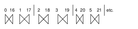
In addition to changing the access patterns so as to achieve data locality, we are also changing the order in which the various operations of the FFT are carried out. Figure 16 illustrates pictorially the first few operations of the FFT before any data restructuring has taken place. The operation of, say, combining elements and to give the new values for and , in place (i.e. without the need for temporary arrays) is called the “butterfly” because of the way it is traditionally drawn (with vertical and diagonal lines) as in Fig. 16. Even at this stage (before any data restructuring occurs) we carry out the butterfly operations in non-standard order.
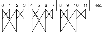
In the traditional FFT, all butterfly operations involving the smallest strides are carried out first before moving to larger strides (e.g. all butterfly operations involving nearest-neighbors such as and are carried out before moving to next-nearest-neighbors such as and etc.). In the new algorithm, however, we want to maximize in-cache operations so we carry out all operations with the first set of data that fits in cache before moving on. This is illustrated in Fig. 16 as follows.
In keeping with the example of the previous subsection we are setting (nominally the cache size for this example). The vertical bars separating groups of four numbers (e.g. ; , etc) schematically indicate cache boundaries. Thus we perform all operations of the FFT (with sequentially increasing strides) within a given data vector of length until the point at which the stride equals . At that point we move the next group and repeat the process until all groups of data have been exhausted. To proceed to the next step (where the stride ) would lead to cache misses for the data structured as in Fig. 16. At this point, therefore, we carry out the reshape-transpose operation to restructure the data.
In the next two cycles of the FFT we work with the re-structured data so as to achieve data locality as illustrated in Fig. 17. Note that the access patterns are identical to those of Fig. 16 and that all operations which can be carried out with a given set of data elements (i.e. those which fit within a vector of length ) are performed before moving on to the next group.
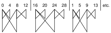
At this point one can see the general pattern emerging. (1) The index-optimized radix- FFT of Fig. 15 is carried out within a given data block of length albeit with modified weights (to be discussed in the next subsection). (2) Then an outer loop cycles over the data blocks. Following that, (3) the data is re-arranged by carrying out a reshape-transpose until the last re-arrangement is achieved. (4) At this point, one must decide how many cycles of the FFT need to be done after the last reshape-transpose as, in general, the number of cycles after the last reshape-transpose might be less than . (5) Lastly the original ordering of the data is restored (as discussed in section 21.2).
In the last paragraph, in step (4), we mentioned that after the final reshape-transpose the number of FFT cycles within a given data block of length might be fewer than for all the other stages of the calculation. This can be clearly seen in the present example. As illustrated in Fig. 18, in the last stage of the present example, only cycles of length are needed (as opposed to cycles of and for previous orderings).
12.3 The Number of Reshape-Transpose Operations
The total number of reshape-transpose operations and the number of FFT steps between reshape-transpose operations is determined by the two parameters and total length of the input data array . The illustrations of the butterfly operations presented in Figs. 16, 17, and 18 illustrate the notion of the stride of the data elements being combined. The stride is simply the number of memory locations separating a given two elements. From the definition of the block matrices (see Fig. 14) we easily identify the stride to be equal to . Since the stride doubles with each iteration of the FFT, we find that a stride of length (the maximum stride which stays within the vector of length ) is reached after steps of the calculation. Thus there are FFT steps between subsequent reshape-transpose operations.
The total number of iterations of the FFT is , therefore the total number reshape-transpose operations is the integer part of the ratio .
12.4 Re-Ordering of the Weights
The book-keeping for the weights required for the new algorithm is presented in this subsection. We wish to implement the new algorithm as a generalization of those illustrated in Figs. 14 and 15. In order to do that we must keep track of which weights go with which elements of the data array as it is re-arranged via the sequence of reshape-transposes.
At this point it is convenient to return to the notation of subsection 11.1 in which we illustrated a given iteration of the FFT as the multiplication of a block-diagonal matrix by an -dimensional vector. As discussed in the previous subsection, we carry out iterations of the FFT (the last of which having a stride ) and then re-arrange the data with a reshape-transpose operation. Then we carry out another steps before re-arranging, etc. Thus the last iteration before the first reshape-transpose is written as:
| (63) |
Thus the first operation requiring the use of the restructured data is written as:
| (64) |
Let us write the reshape-transpose operation as a linear transformation defined by the matrix acting on the data vector as
| (65) |
where we have introduced the notation to indicate the data as re-ordered by the reshape-transpose operation. Next we transform Eq. 64 by multiplying both side of the equation, on the left, by the matrix and introducing the identity between the matrix and the vector to give:
| (66) |
which, in turn we write as:
| (67) |
In equation 67 we have introduced the re-ordered weight matrix:
| (68) |
which defines the first iterate of a sequence of transformations involving the re-structured data. We have also introduced the first-iterate data vector .
This iterative procedure continues in an analogous fashion to that outlined in subsection 11.1 using the matrices for . The last step in this sequence of operations (i.e. before the next reshape-transpose is carried out) is given by:
| (69) |
where .
At this point we introduce the next restructuring of the data and transform the next step of the FFT as:
| (70) |
and the procedure continues in an obvious fashion.
12.5 -Reduction
As emphasized in subsection 11.1 we never actually materialize (instantiate) any matrices. The discussion of subsection 11.1 and of the previous subsection is merely for the purpose of constructing the derivation. Ultimately we use the techniques of the -calculus, in particular the technique called “-reduction” to arrive at an implementation analogous to that of Fig. 15. The process of -reduction is a procedure which reduces an algebraic expression to its simplest form by eliminating temporary arrays. In effect, all array access operations are effected through direct indexing. The application of this procedure to the general-radix FFT is discussed in Ref. [19] and the result for the special case of the radix- FFT is presented in Fig. 15
In order to effect the -reduction for the present problem we must consider the structure of the transformed weight matrices, such as (for ) in greater detail as presented in the next subsection.
12.6 Structure of the Weight Matrices
In this subsection, we consider the structure of the weight matrices and the corresponding transformed weight matrices in some detail. As discussed in subsection 11.1, the matrix is a block-diagonal matrix, consisting of , -dimensional blocks . The structure of the block matrices is given in Fig. 14. Note, each of the block matrices is sparse, having only non-zero elements. The remaining elements are zero. Note, by using -calculus techniques, we only carry out multiplication operations involving non-zero elements.
The effect of the reshape-transpose operation on the weight matrix is to rearrange each of its sparse diagonal blocks into a series of smaller diagonal blocks. Thus through the repeated use of the reshape-transpose operation the weight matrix remains banded with a fixed maximum width dictated by the parameter .
12.7 Transforming the Weights
The non-zero elements in a given block map a specific set of elements of the data array into the corresponding elements of the updated array. There is thus a unique homomorphism of the nonzero elements of the array and the elements of the data vector. The non-zero elements of a block are contained within four -dimensional sub-blocks (see Fig. 14). Two of these blocks are the -dimensional identity matrix (in Fig. 14 ) . The other two blocks consist of the -dimensional blocks , and .
The transformation of the weight matrix can be determined by constructing a unique isomorphism between the non-zero elements of and the elements of the data vector . Since we know how to transform the data vector using the reshape-transpose, the isomorphism allows us to determine the transformation of the weight matrix.
The isomorphism is very simple. We begin by constructing a vector of length as follows. The first elements are unity, taken from the identity matrix of the first block . The next elements are the non-zero elements (taken in lexical order) of the matrix also from the first block . The next elements are unity taken from the second block , and the next elements are the non-zero elements of also from the second block . This procedure continues until elements have been extracted from each block to yield the -dimensional weight vector . This procedure is completely general and applies to all transformations of the weight vector. Before the first reshape-transpose all of the blocks are identical. However, as we will see, for all other weight matrices generated by the reshape-transpose operation, the sub-blocks will in general be different.
The vector transforms in the same way as the data vector to give a transformed weight vector. Thus we only need to keep track of the changes to the weight vector under the influence of the reshape-transpose operation. We follow the procedure to transform exactly as was done to transform . That is we re-shape it into a two-dimensional vector and observe the re-ordering which occurs due to the reshape-transform operation.
That the isomorphism between and is correct can easily be seen by the following argument. In carrying out one butterfly operation, we update the data vector two elements at a time. For the -th FFT step, the stride is and therefore elements and are combined with the corresponding weights in the array as follows
| (71) |
and
| (72) |
Since each element of gets multiplied by the corresponding element of the two vectors must transform together. Again we emphasize that the multiplications by unity implied in the first terms of Eqs. 71 and 72 is only an intermediate step in the derivation. In the final implementation there is no multiplication by unity or zero.
13 Cache-Optimized FFT Illustrated
13.1 Specific Examples and Patterns
Consider now the transformed equation as defined by Eq. 68. The matrix to be transformed, is a block-diagonal matrix with , blocks . Each matrix , is thus comprised of two -dimensional identity matrices and two -dimensional matrices and . As indicated in Fig. 14, is a diagonal matrix with elements (i.e. the (2c)-th root of unity raised to the -th power) for . Thus the elements of the weight vector consist of: (1) entries equal to unity, (2) , -th roots of unity: , , (3) entries equal to unity, etc. Now upon reshaping the weight vector we obtain:
| (73) |
Returning to our example of the array, explicitly, we have:
| (74) |
Now reorder with a reshape-transpose to give
| (75) |
Now by reversing the process that was used to construct the weight vector from the elements (which is in this example) we obtain from the weight vector the weight matrix :
| (76) |
13.2 Structure of Reshape-Transposed Weight Matrix
Note carefully the structure of given in Eq. 76. The equation is now block diagonal with blocks along the diagonal. Thus the access patterns for the matrix multiplication
| (77) |
using the reshape-transposed quantities are the same as those for
| (78) |
Now, however, we must realize that the structure of is more general than that of
Previously, in the definition of the untransformed matrices , a block diagonal sub-matrix was completely specified by its dimension . Now however, the definition of the sub-matrices must be generalized.
We see in Eq. 76 that the first four blocks on the diagonal are equal and the weight element is the same as that we previously found in the definition of the sub-matrix (see Fig. 14). Now, however, there are four different matrices. They are distinguished by their weight elements , , , , respectively.
Now we see that the weight matrix, requires three labels: (1) to determine the particular root of unity ( in this example), (2) giving the power of the root, (, , , and in this example), and (3) ( in this example) to determine the dimensionality (this in turn, is related to the number of reshape-transpose operations which have occurred). We use the symbol , which is a -dimensional matrix. Likewise we generalize the definition of the block sub-matrices . For example:
| (79) |
So far we have only encountered the -dimensional () weight matrix . The generalization to higher dimensions (which depends on how many times the reshape-transpose operation has occurred) will be presented shortly.
We now summarize the discussion of for the case. The block diagonal matrix to be transformed, , consists of four identical -dimensional blocks . We write:
| (80) |
The transformed matrix, on the other hand, transforms into four groups of four different matrices:
We now state the result for the next iterate of the weight matrix , and then illustrate it in detail. The matrix is a sparse matrix () consisting of four groups of two, matrices as:
where the four-dimensional weight sub-blocks are given by
| (83) |
Note that the sequence of matrices , for ( for this example) in Eq. contain all of the weights: , , , , , , , , originally present in the untransformed matrix
13.3 Derivation of From the Weight Vector
We now explicitly illustrate the construction of the weight matrix from the corresponding weight vector . As was discussed for the situation illustrated by Eqs. 73 and 74, we form the weight vector from the elements of and reshape to give:
| (84) |
Next we carry out the reshape-transpose to give:
13.4 Last Step
The last step in this example () corresponds to the original weight matrix :
| (86) |
Carrying out one reshape-transpose gives:
which is a block-diagonal matrix consisting of blocks. One can see that Eq. is the analog of Eq. 80. In order to achieve data locality (i.e. blocks of dimension less than or equal to ) we must reshape-transpose once more to yield:
which is a block-diagonal matrix with sixteen different sub-blocks on the diagonal.
14 The General Algorithm
The general pattern for the multiply-restructured weight matrices was discovered, by continuing the analysis of the past few sections with larger and more general data structures, and is presented in this section.
14.1 Numbering
There are operations before the first reshape-transpose corresponding to strides of length , where we allow . For iteration the block-diagonal sub-matrices of have dimension .
After the first reshape-transpose the block-diagonal sub-matrices of array , for are of dimension as before, however there are now different types of weight matrices which must be specified, in addition to their dimension, by a parameter .
At this point, the length of the FFT cycle is which also denotes the root of unity (e.g. , and powers thereof). Because the number of distinct roots of unity (i.e. ) is greater than can fit in a single vector of length there are different types of block sub-matrices for a given dimension. There will also be copies.
We find it convenient to specify the cycle length with two parameters and where we define where for , the variable cycles through the values . After the first reshape-transpose, and we write for , after the second reshape-transpose we have , and , etc. Thus the variable counts the number of reshape-transpose operations.
14.2 General Weight Sub-Matrices
After reshape-transpose operations, the weight matrix is most-conveniently specified by including as an additional parameter. We designate the weight matrix with four parameters: (the type of matrix), its dimensionality, the root of unity, and the number of reshape-transpose operations which have been carried out. Explicitly we have,
| (89) |
where the -th component of the (diagonal) matrix is given by:
| (90) |
where , and the number of different types of matrices is indicated by .
14.3 Number of Different Weight Matrices
The number of different weight matrices is determined as follows. We specify the total data array length by . With this factorization we have by definition We use two parameters to specify the cycle length where counts the number of transposes and (indices and cycle as inner and outer loops respectively). For all the variable cycles as . For , we have the restriction
Next determine the number of different cycles:
| (91) |
This is to be interpreted as the number of different weight matrices of dimension . For cycle lengths we find and meaning that for this case (corresponding to the traditional FFT without reshaping) each matrix is uniquely determined by its dimensionality.
Note also that the number different weight matrices jumps by a factor of for each reshape-transpose operation. For example, after the first reshape-transpose operation, we have different matrices corresponding to factoring the cycle length . For the next FFT iteration we have corresponding to , which becomes factored as different matrices etc. After the next reshape-transpose operation there are different weight matrices of a given size where as before and cycle length .
14.4 Number of Copies of a Given Cycle Length
The number of copies of a given cycle length is given as the ratio of the total data vector length to the cycle length :
| (92) |
To shed some light on this quantity, consider the situation we encounter on the last step of the FFT in which . In this case and there is only one copy of each weight matrix . For example if then we have the total data vector length and we have each of the different matrices represented only once. If on the other hand we have we have and each of the different matrices appears only once etc.
Next consider the situation in which . In this case and there will be two cycles and each matrix appears twice.
The algorithm can be thought of as a generalized FFT algorithm which processes vectors of length . The weight matrix thus naturally partitions into blocks. Thus we must consider the total number of copies of a given block. This is computed as follows. The length of a given set of copies is which is partitioned into blocks of length is obtained by dividing by to give:
| (93) |
15 Cache-Optimized FFT Using the -Calculus
At this point we turn to a brief look at two key steps in the algorithm: the reshape-transpose and the final transpose. These two examples serve as vehicles to illustrate the use of Conformal Computing techniques. The discussion here presents only the key results. The complete details of the derivations are presented in the following chapter (part II).
15.1 Reshape Transpose Operation
Recall the expression to abstract our view of the cache. We write:
| (94) |
to represent the reshape-transpose operation on our restructured data array. Reading from right to left we start with the array of indices which is a one-dimensional array (vector) of sequential integers starting with and ending with . In the present example we only concern ourselves with the manipulation of this index array. The first reshaping of () is indicated in Eq. 104 by the expression which implies a array consisting of the entries of taken in sequential (i.e. row-major) order. For this example we require the reshaped array to contain the same number of elements as the original array: . Using the notation of the we write , where the operator acting on a vector produces a scalar equal to the product of the elements of the vector.
In the next step in Eq. 104 we apply the transpose operator to produce the array . In the last step we re-partition the array with the to produce the array obtained by taking the elements of sequentially in lexical order (i.e. row-major).
15.2 -Reduction of the Reshape-Transpose Operation
Using Conformal Computing techniques, an Operational Normal Form (ONF) is obtained from Eq. 104 as is derived in detail in Part II. For the purposes of this paper we merely indicate the final result. The ONF is an algebraic specification, in terms of indices (i.e. starts, stops and strides), that indicates explicitly how a given expression is to be built (in software or hardware). For simplicity we define:
| (95) |
Using this notation we express the ONF of Eq. 104 as:
| (96) |
| (97) |
The last step that expresses the result directly in terms of the elements of the array (as opposed to ) is discussed in detail in the next chapter (Part II). The result is simple and has been directly translated into C++ code as indicated in Fig. 28.
void trans_rshp(complex *datvec,complex *temp,int nmax,
                int csize)
{
        int iind,jind,kind,kmax,jmax,imax,index,c2size;
        int rows,arg;
        int max(int a,int b);

//      The routine carries out the transpose-reshape operation
        index=0;

        rows = nmax/csize;
        imax = rows-1;

        c2size = int(pow(csize,2.0));
        jmax = max(0,nmax/c2size-1);


        for(jind=0;jind<=jmax;jind++)
        {
            for(iind=0;iind<=imax;iind++)
            {

                temp[index] = datvec[jind+csize*iind];
                index += 1;
            }
        }

        for(iind=0;iind<=nmax-1;iind++)
        {
            datvec[iind] = temp[iind];
        }
}
15.3 Reordering the Data
After the last step of the FFT the data will not be in the correct order and we must do something to return it to its initial order (i.e. prior to any reshape-transpose operations). The simplest approach would be to rearrange the data by applying a series of inverse reshape-transpose operations. There is, however, a far more efficient approach in which no data needs to be moved. In other words, we use Conformal Computing techniques to determine the index vector which will select the correct components of the array. We present only the final result in this paper. Complete details of the derivation and an in-depth discussion (with examples) is presented in the following chapter (Part II.).
The input data vector of length is carried into the vector through the steps of the FFT. In the process, reshape-transpose operations have been carried out. The resulting vector is thus not in the correct order (as a result of the multiple reshape-transpose operations) and must therefore be rearranged into its final form . We now obtain as
| (98) |
where and and is the rotate operator that induces a cyclic permutation of the vector (as will be discussed in detail in Part II). The operators acting on the vector , in Eq. 162 represent the composite inverse operation of the series of reshape-transpose operations that occurred during the FFT. In the final step, we reshape into a one-dimensional array:
| (99) |
The ONF is now expressed as follows. Define two new indices and with limits given by:
| (100) |
and,
| (101) |
we define a new two-dimensional array by reshaping the vector as:
| (102) |
The final result is then written:
| (103) |
This expression was directly translated into C++ code as illustrated in Fig. 29.
void final_trans(complex *datvec,complex *temp,int nmax,
                 int lcap,int csize)
{
/*      dvar = # of 2’s in the hypercube
 *      lcap = # of transpose-reshapes (T-rho) that have to be undone
 */
        logc = log(float(csize))/log(2.0);
        sig = lcap*logc;
        smax = pow(float(2),sig);

        dvar = log(float(nmax))/log(2.0);
        tmax = pow(2.0,dvar-sig);

        index = 0;
        for(tind=0;tind<=tmax-1;tind++)
        {
            for(sind=0;sind<=smax-1;sind++)
            {
                temp[index] = datvec[sind*tmax + tind];
                index += 1;
            }
        }

        for(index=0;index<=nmax-1;index++)
        {
            datvec[index] = temp[index];
        }
}
16 Results and Discussion
The performance results for our new algorithm are presented in Figs. 30 and 31. These experiments were run in a single-processor, dedicated, non-shared environment on the IBM SP2 machine “squall” at the Maui High-Performance Supercomputer center [58]. Specifications for the machine are quoted in the caption to Fig. 30.
In the first figure (Fig. 30) we plot the time vs. input data length. There are two curves, one for our new cache-optimized FFT and one for a similar run with no cache optimization. Direct comparisons are possible since both curves are produced by the same code. For the non-cache-optimized run, we simply chose the blocking size (specified as a parameter at run time) to be greater than or equal to the length of the data vector . We see that the curves have essentially the same shape but the cache-optimized one is shifted to the right by one power of two compared to the non-optimized one. Thus for a given run time, we can legitimately claim a factor of two speed-up.
The results presented in Fig. 31 emphasize the improved performance for a fixed data size by taking the ratio of the run time for the non-optimized run to the cache-optimized one. We see that for the some of the largest sizes considered, a factor on the order of speedup is achieved.
Figure 31 is also enlightening in that it highlights the various levels of the memory hierarchy. A change in slope of run-time vs. size indicates the crossing of a boundary between one level of the memory hierarchy and another. For example from the results of Fig. 31 we can make the following estimates. For roughly the speed is most likely dominated by the speed of the registers. For the speed is dominated by L1 and L2 cache and for the speed corresponds to main memory. For paged memory (of size ) dominates. The large jumps in performance (i.e. factors of for the largest sizes) correspond to the presence or absence of page faults.
In general, the performance of the algorithm is a tradeoff between the increased speed obtained by having more data in the cache (with increasing ) and the cost of actually moving the data around. One might naively guess that the best performance would be obtained by choosing to be equal to the cache size. However, we find, the best performance by choosing blocking sizes given by small powers of . In other words, it is more economical to move data around many times within the cache than it is to move large blocks into and out of cache due to the extreme speed of the cache. That is, direct access and movement of components within the cache has no overhead.


17 Conclusions
We have presented a new algorithm for the Fast Fourier Transform that is a
factor of to times faster than our previous records
(that were competitive with or outperformed well-tested library routines as
shown in Chap.
Conformal Computing: Algebraically connecting the hardware/software
boundary using a uniform approach to high-performance computation
for software and hardware applications
SPIN Springer’s internal project number, if known and Ref. [19]). This success was
achieved through the use of Conformal Computing techniques to devise a
generalized partitioning scheme leading to optimized cache access. The
principle is very simple. Data is periodically re-arranged so as to always
achieve locality in cache. This approach is in contrast to the traditional FFT
in which data access becomes progressively remote (leading to cache misses
and page faults) as the algorithm proceeds. The key concept in the new
algorithm is the repeated use of the reshape-transpose operation
to move data from remote locations into the cache as needed. A given
one-dimensional data structure for the input vector is initially reshaped
into a two-dimensional array of dimension where is an
arbitrary blocking size. The blocking size is completely arbitrary and
is specified as a parameter at run time. Based on various cost functions
(cache speed, cost of moving data, etc.) we can predict the performance
of the algorithm vs. the blocking size . We find the best performance
for blocking sizes given by small powers of . The results presented in
this paper are promising for further developments in terms of optimizations of
multi-dimensional FFT’s over cache in single as well as multi-processing
environments.
Chapter \thechapter A Cache-Optimized Fast Fourier Transform: Part II
18 Chapter Summary
This chapter explores in detail two key steps of a new cache-optimized
Fast Fourier Transform algorithm that was presented in the previous chapter
(see Chap.
Conformal Computing: Algebraically connecting the hardware/software
boundary using a uniform approach to high-performance computation
for software and hardware applications
SPIN Springer’s internal project number, if known).
Through the use of Conformal Computing techniques, discussed herein, an
impressive performance improvement (factors of to speed-up) was
obtained. The present chapter serves as a tutorial introduction to the
techniques of Conformal Computing: a systematic design methodology for
hardware/software
algorithms based on a rigorous mathematical theory. Two key aspects of the
new algorithm, the reshape-transpose and final-transpose are
explored in detail, and serve as vehicles to introduce and illustrate many
key aspects of the theory. Although our approach is based on a rigorous
formal theory, the net result is always an efficient specification, the
Operational Normal Form (ONF) for how to build a particular algorithm in
software or hardware in any programming language. As we explicitly
demonstrate, the ONF for each of the operations (reshape-transpose and
the final-transpose) are directly translated into computer code.
19 Introduction
This chapter continues the discussion of the cache-optimized FFT presented in
the previous chapter (Part I: see Chap.
Conformal Computing: Algebraically connecting the hardware/software
boundary using a uniform approach to high-performance computation
for software and hardware applications
SPIN Springer’s internal project number, if known) and develops the
techniques of Conformal Computing in
some detail. Over the past decade, these techniques have been successfully applied
to a number of algorithms that are ubiquitous across science and
engineering disciplines, such as the Fast Fourier Transform
(FFT) [16, 19, 17, 18, 59], LU
decomposition [60], matrix multiplication, Time Domain convolution,
QR decomposition [20, 61], etc. That is to say, these and other
algorithms were first expressed algebraically using MoA then -reduced.
These designs were realized in both hardware and
software [62, 63, 64, 65, 66, 67, 68, 69].
At this point we turn to a detailed look at two key steps in the new cache-optimized FFT algorithm: the reshape-transpose and the final transpose.
20 Reshape Transpose
20.1 Algebraic Specification
Recall the expression to abstract our view of the cache. We write:
| (104) |
to represent the reshape-transpose operation on our restructured data array. Reading from right to left we start with the array of indices which is a one-dimensional array (vector) of sequential integers starting with and ending with . In the present example we only concern ourselves with the manipulation of this index array. The first reshaping of () is indicated in Eq. 104 by the expression which implies an array consisting of the entries of taken in sequential (i.e. row-major) order. For this example we require the reshaped array to contain the same number of elements as the original array: . Using the notation of the -calculus we write , where the operator acting on a vector produces a scalar equal to the product of the elements of the vector.
In the next step in Eq. 104 we apply the transpose operator to produce the array . In the last step we re-partition the array with the to produce the array obtained by taking the elements of sequentially in lexical order (i.e. row-major).
20.2 -Reduction: Denotational Normal Form and Operational Normal Form
As we will see in the following, all of the operations in Eq. 104 are composed to yield one final expression through the use of direct indexing. The process of converting an expression such as that in Eq. 104 into one involving only indexing operations is called -reduction. The first step is to produce the Denotational Normal Form (DNF) which reveals the semantic meaning of a reduced array expression such as Eq. 104, in terms of Cartesian coordinates.
For example, given an array A, we write:
| (105) |
where we’ve introduced the operator which takes an index vector and extracts the -th element of the array . On the right hand side of Eq. 105 we use a common bracket notation to denote a component of an array. For an expression involving a number of operations, such as the one in Eq. 104, the DNF is obtained by composing indices using the operator and an index vector by applying the definitions of the various operations (, , etc.) as will be demonstrated shortly. In essence, we view each operator (, , etc.) as effecting a certain re-arrangement of the index vector. Obviously such re-arrangements can be performed sequentially to find the re-arrangement corresponding to the composite operation. The resulting expression, involving only the starting data array (i.e. the array in this example) and Cartesian coordinates is, by definition, the DNF which is independent of layout.
The final step of the -reduction process results in the Operational Normal Form (ONF) which describes the underlying access patterns of the array operation in terms of the specific data layout1010 10 In this context, layout means row major, column major, regular sparse, etc. on a computer. Explicitly, for the simple example of Eq. 105, we write:
| (106) |
if the layout is row major, and
| (107) |
if the layout is column major. Equations 106, and 107 are examples of ONF’s corresponding to the DNF of Eq. 105. By necessity, the ONF is dependent on the underlying data layout as are the operations reshape and ravel ( rav ).
In Eqs. 106 and 107 the operation rav (which we call ravel) produces the one-dimensional vector from the elements of the array . The ordering of the elements of depends on the layout (row-major vs. column-major). For an array A in row-major order, the first elements of are the elements of the first row, the next elements of are taken from the elements of the next row etc. In a similar way, if A is an array, in column-major order, the first elements of are taken from the first column of A, the next from the second column of , etc.
In Eqs. 106 and 107 we have also introduced the layout
functions,
, and
which produce scalar indices in order to
extract a single element from the one-dimensional array .
In general there will be a family of layout functions for various situations.
Equations 106 and 107 are each, therefore, of the form
| (108) |
where is a scalar, and we have again used the bracket notation (as is done in ) on the right hand side of Eqs. 106, 107 and 108 to denote the use of a scalar index to extract a component of a one-dimensional array.
The indexing functions and take two arguments: (1) the index vector and (2) the shape vector . The shape vector is a vector consisting of the lengths of the various dimensions of the array. For the present example, given an array , we have:
| (109) |
The function was given in Definition 1 and in all further discussions we will assume row-major ordering and drop the subscript:
20.3 From the ONF to the Generic Design
The ONF describes how to build the code independent of a particular programming language. At this point all loop nests are revealed, and all data flow and memory management are indicated. Each loop nest indicates not only access patterns but levels of the processor/memory hierarchy. We use (for all) as our generic loop indicator. Similarly, bracket notation indicates “address of” so that when indices are calculated they are calculated relative to the address of the indicated array (i.e. the address of (pointer to) the first element). All of this in conjunction with gives us all essential information to build the design in any programming language at both the hardware and software levels. For example,
| (110) |
denotes a generic form with two loops with in the body. At this point a mechanization to any language is possible. Similarly, loops indicating message passing, shared memory access can easily be instantiated by whatever libraries support that loop level.
20.4 -Reduction of the Reshape-Transpose Operation
We now return to the problem of -reducing the reshape-transpose operation of Eq. 104. To illustrate this example we choose , and , as was done in earlier discussions.
20.4.1 Step I: Determine Shape
The first step in the -reduction process is the determination of the shape vector which, for this example, is given by:
| (111) |
This step is crucial in order to enforce the use of valid index vectors. In order for an index vector to be valid, its components must not exceed the lengths of the corresponding dimensions of the shape vector. Specifically we say that a valid index vector satisfies:
| (112) |
where the notation and implies component-wise comparison of the two vectors and .
20.4.2 Step II: Perform Psi-Reduction and Reduce to Normal Form(s)
We begin by taking Eq. 104 apart using the operator and an index vector . To simplify the notation we define the quantity within the innermost set of parentheses in Eq. 104 as . By applying the definition for reshape: , we get:
| (113) | |||||
In Eq. 113 we are applying the definition of the reshape operator to the object which is defined in terms of the function. In the first line of Eq. 113 the expression: , is part of the definition which handles the case in which one wants to reshape a smaller array into a larger array from the elements of the smaller array (repeated appropriately). In this case, however, the total number of components in the reshaped array is the same, allowing us to drop the expression, , in the second line of Eq. 113. In the third line of Eq. 113 we have inserted the explicit expression for from its definition (see Definition 1).
Next we wish to get rid of the transposed array in favor of the original array . We consider selecting an element of using an index as follows:
| (114) |
| (115) |
In order for this expression to agree with Eq. 113 we must equate the arguments in square brackets in Eqs. 113 and 115 as:
| (116) |
From this we find the the primed indices in terms of the unprimed indices (assuming for this example) as:
| (117) |
and,
| (118) |
20.4.3 Step III: further Simplification
The formulation just presented, while formally correct, is computationally inefficient. In particular, we wish to avoid the operations int and in Eqs. 117 and 118. Instead, if we need to work with both the primed and un-primed indices we can use the loop structure (expressed in C++ syntax assuming for this example) given in Fig. 23:
i = 0;
ratio = r/c;
for(iprime=0;iprime < c; iprime++)
{
   for(k=0; k < ratio; k++)
   {
      for(j=0; j < c; j++)
      {
         jprime = j + k*c;
      }
      i = i + 1;
   }
}
In our applications, further simplification occurs. Note, in Eq. 113 a single element is extracted from the transposed array . In this case, as in many situations, we can compute the entire and select elements from it.1111 11 Bear in mind: in our cache-optimized FFT we actually materialize so as to achieve data locality. As such it is most efficient to compute all at once. This is most easily computed by looping over the values of the index in the rightmost expression in Eq. 119.
Thus, to construct the array
| (120) |
for example, we only need the elements of the corresponding one-dimensional array:
| (121) |
constructed from Eq. 119
This computation was implemented in C++ as illustrated in Fig. 24. Note in Fig. 24 the two for-loops correspond to the bounds as indicated in Eq. 114 upon making the substitutions:
| (122) |
and,
| (123) |
This substitution is made to simplify the notation and is allowed because: (1) the bounds on (see Eq. 114) coincide with those on (see Eq. 112) and, (2) we are constructing the entire array and we need not keep track of the explicit relationship between the primed and unprimed indices indicated in Eqs. 117 and 118.
Note also that the argument of datvec on the right hand side of the assignment temp[index] = datvec[jind+csize*iind]; in Fig. 24 is a direct translation of the argument that appears in Eq. 119 upon carrying out the substitutions of Eqs. 122 and 123.
void trans_rshp(complex *datvec,complex *temp,int nmax,
                int csize)
{
        int iind,jind,kind,kmax,jmax,imax,index,c2size;
        int rows,arg;
        int max(int a,int b);

//      The routine carries out the transpose-reshape operation
        index=0;

        rows = nmax/csize;
        imax = rows-1;

        c2size = int(pow(csize,2.0));
        jmax = max(0,nmax/c2size-1);


        for(jind=0;jind<=jmax;jind++)
        {
            for(iind=0;iind<=imax;iind++)
            {

                temp[index] = datvec[jind+csize*iind];
                index += 1;
            }
        }

        for(iind=0;iind<=nmax-1;iind++)
        {
            datvec[iind] = temp[iind];
        }
}
21 Reordering the Data
After the last step of the FFT the data will not be in the correct order and we must do something to return it to its initial order (i.e. prior to any reshape-transpose operations). The simplest approach would be to rearrange the data by applying a series of inverse reshape-transpose operations. There is, however, a far more efficient approach in which no data needs to be moved. In other words, we use Conformal Computing techniques to determine the index vector which will select the correct components of the array.
21.1 Final Transpose
We now seek to answer the following general question: after a single reshape-transpose operation, where is the data? More precisely we are interested in the re-arrangement of the corresponding index vector. The answer to this question was revealed to the authors upon viewing the data vector as an -dimensional hyper-cube. The hyper-cube is formed by reshaping the data into an array where the number of -s is given by . An element of the hyper-cube is then determined by specifying an index vector of length consisting of ones and zeros. There is, therefore, an isomorphism between the index vector of an element and the binary number corresponding to the index of the original one-dimensional array.
For example, suppose , then the original data vector would be:
| (124) |
Next we re-shape this vector into a hyper-cube by performing the following operation
| (125) |
The operation in parentheses yields
| (126) |
which is the argument to the second reshape operator. Thus more explicitly, Eq. 125 is written as:
| (127) |
which is a array constructed by taking the elements of in increasing order.
Incidentally, the operation of Eq. 126 is an example in which a smaller array (in this case the scalar ) is reshaped into the larger array . Such a situation was anticipated in the definition of the reshape operator by the presence of the modulo operation (e.g the factor in Eq. 113), as was discussed earlier in the context of Eq. 113.
The elements of the hyper-cube are now selected by specifying an index of zeros and ones corresponding to the binary representation of the original array. For example:
| (128) |
| (129) |
etc., where we have again used the bracket notation to denote selection of elements of one-dimensional arrays.
Unfortunately, there is no truly satisfactory way to visualize the hyper-cube construction. However, for the purpose of discussion, we have adopted the following convention. We begin by grouping four elements together at a time and write them as matrices surrounded by square brackets. For example suppose we have a -dimensional hyper-cube defined by
| (130) |
the first four elements of would be written as:
| (131) |
where we have used a partial index to select the first four elements of : , , , and we have written them as a two-dimensional array (assuming row-major order). the next four would be grouped together as:
| (132) |
followed by
| (133) |
and lastly:
| (134) |
The entire array can thus be visualized by arranging the four blocks as a array of arrays and enclosing them in parentheses as:
| (135) |
The generalization to higher dimensions is straightforward. In the present example we are assuming the hyper-cube to be of even dimension (i.e. ). For an odd-dimensional hyper-cube, we treat the final index (on the left) as defining a column index.
For example, consider the array defined
to be the last step in the FFT for the example given in
Eq. 62 in Chap.
Conformal Computing: Algebraically connecting the hardware/software
boundary using a uniform approach to high-performance computation
for software and hardware applications
SPIN Springer’s internal project number, if known.
| (136) |
Our task in the next section is to correctly identify an index vector which rearranges Eq. 136 into the correct order (i.e. ascending integers starting with ) without actually moving any data.
21.2 General Rule
By studying the patterns induced by the reshape-transpose operation on arrays arranged as hyper-cubes (such as that in Eq. 136), the authors have discovered a rule for returning a hyper-cube of any dimension (e.g. an input data vector for an FFT of any length) to its correct form in one step through the use of indexing, without the need to actually rearrange the data. We present and discuss this rule in this section. The rule is simply stated as follows.
Given an array , that has been rearranged with the reshape-transpose operator to give , we select an element of with a binary index of the array formulated as hyper-cube. The element, so selected, is obtained from the array (also formulated as a hyper-cube) with the index where is simply a cyclic permutation of .
At this point, we present an example to clarify the situation. Consider a array of integers starting with and ending with which is written as
| (137) |
Now define the array obtained through a reshape-transpose operation acting on :
| (138) |
Incidentally, for the special case of a square array (as we are considering here) the reshape-transpose operation is equivalent to the transpose operation.
Let us now reshape the arrays as hyper-cubes, that is:
| (139) |
and,
| (140) |
Now if we consider the relationship between the elements of and viewed as hyper-cubes we find the following behavior:
| (141) |
For example:
| (142) |
| (143) |
| (144) |
The general rule is as follows. Suppose there are , ’s in the hyper-cube representation of an array (with ). Upon transforming into via the reshape-transpose operation,
| (145) |
we find the following relation between the hyper-cube representations of and :
| (146) |
where the relationship between indices and will be discussed shortly. In Eq. 146 and are defined by:
| (147) |
and,
| (148) |
To complete the specification of Eq. 146 we need to determine the index in terms of . In general, is a cyclic permutation of in which elements of are sequentially removed from the left and placed at the right. For example, if , and , for
| (149) |
indexing the array , the corresponding index of is given by:
| (150) |
Using the formalism of the -calculus, we rewrite Eq. 150 as
| (151) |
where we have introduced the rotate operation . Naturally we are also interested in the inverse operation which is written as
| (152) |
Now that we understand the relationship between and we are in a position to specify how can be re-ordered to correspond to the ordering of . In order to do that we invoke the definition of the generalized transpose operation .
Up to this point we have only used in its traditional manner for two-dimensional arrays. For an -dimensional array, such as or the transpose operation invokes a permutation of the dimensions which is specified by a permutation vector as its left argument (by convention no left argument is required for two-dimensional arrays). Thus, because we found the following relationship between the components of and
| (153) |
we say that is related to through the following generalized transpose:
| (154) |
and invoking the inverse of this transpose, we can write
| (155) |
In anticipating further developments, we use the rotate operator to write the index vectors more abstractly in terms of the operation. Specifically, Eqs. 154 and 155, respectively become:
| (156) |
and,
| (157) |
The right sides of Eqs. 154 and 155 can be further abstracted by substituting the definitions of and from Eqs. 139 and 140 to yield
| (158) |
and,
| (159) |
We now consider a general array having components. Now define the array to be that which is obtained from through the application of reshape-transpose operations:
| (160) |
we interpret the operator to mean the operation carried out times. Based on the principles introduced so far, the elements of are related to the elements of through the relation:
| (161) |
where and .
21.3 -Reduction
Building on the developments of the previous section, we now show how to effect the final rearrangement of the FFT. In other words, we wish to find the inversion of an equation of the form given in Eq. 161. This is easily accomplished by simply changing the sign of the variable as was demonstrated in Eqs. 156 and 157, a fact which nicely underscores the power of the Conformal Computing approach.
The input data vector of length is carried into the vector through the steps of the FFT. In the process, reshape-transpose operations have been carried out. The resulting vector is thus not in the correct order (as a result of the multiple reshape-transpose operations) and must therefore be rearranged into its final form . We now obtain as
| (162) |
where and . The operators acting on the vector , in Eq. 162 represent the composite inverse operation of the series of reshape-transpose operations that occurred during the FFT. The final step is obtained by reshaping into the final one-dimensional array:
| (163) |
The derivation to normal form follows:
21.3.1 Step I: Determine Shape
We now wish to carry out the process of -reduction of an expression of the form:
| (164) |
The first step is to find the shape () in order to enforce the use of valid indices. The shape is given by:
| (165) |
which shows that permuting the elements of the shape vector does not change the shape of a 2-cube (i.e. a -dimensional hyper-cube. This is true in general for a d-dimensional n-cube). More explicitly, the vector of Eq. 165 is a vector consisting of entries each given by the integer . Such a shape implies that the expression in Eq. 164 is a -dimensional array, the length of each dimension being precisely . In other words it is a -dimensional hyper-cube.
21.3.2 Step II: Perform Psi-Reduction and Reduce to Normal Form(s)
For an index to be valid it must satisfy:
| (166) |
which states that all of the components of must be less than the corresponding components of the shape vector (i.e. the index vector must consist of ’s and ’s).
We now use a valid index vector to select an element of the expression given in Eq. 164. By doing so we can apply the definition of the transpose (which is defined in terms of the corresponding rearrangement of the index vector). For the moment we simplify the notation with the definition:
| (167) |
We thus obtain:
| (168) |
which shows that selecting an element of the transposed array with an index is the same thing as selecting an element from the non-transposed array using an index that has been permuted. This is, in essence, the definition of the generalized transpose operation.
Now we further reduce the form of the index vector as:
| (169) |
which explicitly denotes the way in which is built from two fragments of . We have introduced the operations take and drop which select sub-vectors from . Specifically, forms a vector from the last (i.e. rightmost) elements of and is the vector which remains after dropping the last elements of . In the expression on the right hand side of Eq. 169 we have introduced the operation cat which concatenates the two fragments together. Thus Eq. 168 becomes:
| (170) |
To make further progress, we now rely on the concept of a partial index. For example, suppose we have a three dimensional array . An individual component is specified with a valid full index containing three elements such as:
| (171) |
However, we can also extract sub-arrays of by using partial indices. Thus:
| (172) |
is a two-dimensional sub-array, while
| (173) |
is a one-dimensional array. Therefore, the result of selection with a full index can be written as a composition, such as:
| (174) |
Thus the right hand side of Eq. 170 becomes:
| (175) |
The next step is to apply the Psi Correspondence Theorem, which specifies the manner in which to construct indexing functions (such as the ’s introduced earlier) from arbitrary full or partial index vectors.
21.4 The Correspondence Theorem (PCT)
We now state the Correspondence Theorem algebraically and then pause to take it apart piece by piece.
Definition 8
Given an array with shape , s.t. , and
| (176) |
The operators tau (), and delta () in Eq. 176 give the number of elements of a vector, and the dimensionality of an array, respectively.
Consider first, the left hand side of Eq. 176. The expression is a sub-array of obtained using the (partial or full) index . For example, suppose is a three dimensional array with shape , and , then we have the two dimensional array: for valid indices , and . In this example and . For this example, we have four such arrays since .
Generally the convenient bracket notation for a one-dimensional vector has the following equivalence:
| (177) |
for some scalar . Often we use standard vector notation for emphasis. We stress, however, that the consistent structure of the algebraic system is designed in such a way that scalars and vectors are simply zero-dimensional and one-dimensional arrays and as such don’t require any special symbols. For convenience, however we often use such symbols as to indicate a scalar and to denote the empty vector. The existence of the empty vector is necessary in order that the scalar has the correct shape . The existence of the empty vector may seem strange to some readers. Its use, however, is necessary in order to have a consistent algebra. The need for the empty vector is analogous to the need for the zero in the set of integers and the empty set in set theory.
Note a related aspect of the theory is often misunderstood by newcomers: a vector is NOT equivalent to a array (i.e. a row-vector in traditional matrix theory) NOR is it equivalent to a array (i.e. a column-vector in traditional matrix theory). In the present theory, these three objects each have different shapes, namely, , and respectively. In traditional matrix theory, the distinction plays no essential role.
Continuing our analysis of Eq. 176, on the left hand side, the operation ravel ( rav ) takes its argument, the sub-array and flattens it into the one-dimensional array . On the right hand side of Eq. 176 the expression is written in the form where is a scalar offset which is added component-wise to the vector to produce the vector index . The components of the index vector are integers which select the components of in lexical order. Explicitly the scalar and vector in Eq. 176 are given by:
| (178) |
and,
| (179) |
respectively. These expressions will be described in detail shortly. First we continue the example of a three dimensional array introduced above.
In the example considered above,
| (180) |
is a one dimensional array consisting of the following elements: , , , , , , etc.
Now the significance of reveals itself. It is the index of the first element of our sub-array . Likewise the vector is a vector of integers starting with which serves as a vector of regularly spaced offsets. The total number of integers in the vector is equal to the number of elements in the sub-array .
The shape vector naturally partitions into two sub-vectors given by
| (181) |
and,
| (182) |
In the first expression counts the number of elements of the partial index and the take operation () forms a vector of length equal to that of the index vector composed of the first elements of the shape vector (i.e. the leftmost elements of ). The second expression forms the corresponding vector of the remaining elements. The product of the elements of
| (183) |
gives the total number of elements of the sub-array and is written as:
| (184) |
Now we complete the description of the vector of offsets by using the iota operation to create the vector of integers as given in Eq. 179.
Likewise, the starting index has a simple explanation. In Eq. 178, the expression
| (185) |
counts the number of sub-arrays that precede the one of interest in the array . Thus, in order to obtain the index of the first element of our chosen sub-array we multiply by the total number of such elements, given in Eq. 184 to give Eq. 178
21.5 Applying the Correspondence Theorem
We now apply the PCT, developed in the previous section, to the expression given in Eq. 175. We begin by writing the right hand side of Eq. 175 in the form required by the theorem:
| (186) |
where the partial index of the PCT has been defined to be
| (187) |
and the array of the PCT has been taken to be the subarray:
| (188) |
We now work out the various quantities appearing in the PCT. The index is chosen to be a full index for the array . From Eqs. 165, 166, and 167 we find the shape of the index to be:
| (189) |
From Eq. 187 we find the shape of to be:
| (190) |
which follows from the definition of drop as applied to Eq. 187. Formally we say:
| (191) |
where the tau operator counts the number of elements in the vector . Next from Eq. 188 we find the shape of to be
| (192) |
which shows explicitly that the index vector is a valid full index for the sub-array as required.
Next we compute the following quantity appearing in the PCT:
| (193) |
We obtain the empty vector because the drop operation is dropping elements from a vector that contains precisely elements. In the next step, the product operator acts on this quantity to give:
| (194) |
In general, the product operator multiplies the elements of a vector to obtain an scalar quantity. The equivalence on the right hand side of Eq. 194 defines the product of the empty vector to be unity.
We have now computed all the quantities needed to evaluate the scalar index of Eq. 178. With the above quantities, the scalar index appearing in the PCT is now given by:
| (195) |
Now we need to compute the offset vector appearing in Eq. 179. In order to do that we form the quantity:
| (196) |
We see that the offset vector contains only one entry . Thus the combination selects only one element. This is because although is a partial index of , it is indexing the subarray . Therefore, the index is a full index of the subarray . This is consistent with the fact that, although we are dealing with a partial index and a subarray it is one step in the overall calculation of the action of on the array , the action of which is to select a single element.
We now summarize the calculation so far. We now have:
| (197) |
Now we can simplify the scalar index of Eq. 195 by noting that as the index cycles through all possible values (in order), the scalar takes on all values from to . We thus define a new variable , and the right hand side of Eq. 197 () simplifies as:
| (198) |
Now, we must apply the PCT again, this time to the quantity
| (199) |
that appears in Eq. 198. In order to facilitate the application of the PCT, we redefine the variables and appearing in the PCT as follows. We write:
| (200) |
and,
| (201) |
where we have used the definition of given in Eq. 167.
We now proceed to evaluate, step by step, the quantities appearing in the PCT based on the new definitions of and given in Eqs. 200 and 201. The shape of the new index is given by:
| (202) |
and the total number of components of is
| (203) |
The shape of is given by
| (204) |
Using these results we have
| (205) |
followed by
| (206) |
and
| (207) |
We now have computed all the quantities needed to evaluate the scalar of Eq. 178. Explicitly we have
| (208) |
We can also simplify this expression by noting that as we cycle through all possible values of the partial index vector , the function takes on all values from to . Thus we define a new variable and we note that s. t. the scalar variable is written as:
| (209) |
Lastly, to complete the application of the PCT to the expression of Eq. 199 we compute the offset vector:
| (210) |
Now we summarize this second application of the PCT. By acting on the expression in Eq. 199 with the ravel rav operator and applying the PCT we obtain:
| (211) |
We see that for each value of , the result of Eq. 211 is a vector of length . Returning to Eq. 198, however, we find that to obtain the final result, we must select a component of Eq. 211 using the index . Thus the final expression in Eq. 198, using Eq. 211, is written
| (212) |
which is simply equivalent to the expression:
| (213) |
which is the final result.
21.6 Summary of Final-Transpose Operation
The ONF is now expressed as follows. Define two new indices and with limits given by:
| (214) |
and,
| (215) |
we define a new two-dimensional array by reshaping the vector as:
| (216) |
where is defined in Eq. 163. The final result is then written:
| (217) |
This result was translated directly into code as shown in Fig.29.
void final_trans(complex *datvec,complex *temp,int nmax,
                 int lcap,int csize)
{
/*      dvar = # of 2’s in the hypercube
 *      lcap = # of transpose-reshapes (T-rho) that have to be undone
 */
        logc = log(float(csize))/log(2.0);
        sig = lcap*logc;
        smax = pow(float(2),sig);

        dvar = log(float(nmax))/log(2.0);
        tmax = pow(2.0,dvar-sig);

        index = 0;
        for(tind=0;tind<=tmax-1;tind++)
        {
            for(sind=0;sind<=smax-1;sind++)
            {
                temp[index] = datvec[sind*tmax + tind];
                index += 1;
            }
        }

        for(index=0;index<=nmax-1;index++)
        {
            datvec[index] = temp[index];
        }
}
22 Conclusions
We have presented a tutorial introduction to the techniques of Conformal
Computing illustrated in the context of the new cache-optimized FFT algorithm
presented in the preceding chapter (Part I: see Chap.
Conformal Computing: Algebraically connecting the hardware/software
boundary using a uniform approach to high-performance computation
for software and hardware applications
SPIN Springer’s internal project number, if known). Two key aspects of the new
algorithm, the reshape-transpose operation and the final-transpose
operation were presented and discussed in detail. These two examples
are excellent vehicles for developing and illustrating the new techniques in
that many of the most important concepts of the theory (such as the notion
of shapes, re-shaping, indexing, the function, the -correspondence theorem, etc.) are presented. Indeed, the
reshape-transpose operation is an extremely important concept which is
applicable in many other situations. In addition, the -correspondence theorem is a cornerstone of the Conformal Computing
approach. It is the key link between the Mathematics of Arrays (MOA),
which provides a means for reasoning about the algebraic properties of
array-based algorithms, and the -calculus which allows one to reduce
an algebraic expression to an explicit form that can be directly translated
into computer code in any computer language.
The Conformal Computing approach
is leading to important new insights by allowing one to view multi-dimensional
arrays, their decompositions and mappings in a unified,
general way. In other words, one can change the
dimensionality of a given array, through the use of the reshape operation
to suit the needs of the application at hand (without necessarily moving the
data). In particular, the
multi-dimensional hyper-cube played an important role in the development
of the insights leading to the final-transpose operation appearing in
the new FFT.
In another ongoing investigation, the use of the hyper-cube
representation is shedding new light on problems related to quantum computing:
an area in which the hyper-cube is a natural data structure in a context
based on two-state qubits (see Chap.
Conformal Computing: Algebraically connecting the hardware/software
boundary using a uniform approach to high-performance computation
for software and hardware applications
SPIN Springer’s internal project number, if known).
Chapter \thechapter A Cache-Optimized Fast Fourier Transform: Part III
23 Chapter Summary
This chapter continues to develop the techniques of Conformal Computing as applied to the Fast Fourier Transform (FFT) that were introduced in the two preceding chapters. In these previous chapters, a new cache-optimized algorithm was presented that was two to four times faster than our previous records (which beat or were competitive with well-tuned library routines). This chapter presents a new hyper-cube representation that is contrasted with that of the preceding chapters. We argue that any arbitrary partitioning of the data over cache, processors, etc. can be efficiently handled in a hyper-cube representation. The rearrangements of the data (virtual or physically-realized) are represented in the hyper-cube in terms of direct indexing, thus avoiding most temporary arrays. Implementation and performance details, presented in the two preceding chapters are also reviewed. In addition to the presentation of this new hyper-cube view, this chapter also serves as a continuing tutorial introduction to the methods of Conformal Computing.
24 Introduction
The focus of this chapter is the formulation of the FFT in a generalized hyper-cube representation using the high-level techniques of the Conformal Computing approach.
The Fast Fourier Transform (FFT) is one of the most
important computational algorithms and its use is pervasive in science and
engineering. The work in this chapter builds on that of the two previous
chapters
in which the FFT was optimized in terms of in-cache
operations leading to factors of two to four speedup in comparison
with our previous records. Further background material including
comparisons with library routines can be found in
Refs. [17, 18, 19, 20] and [16] and in Chap.
Conformal Computing: Algebraically connecting the hardware/software
boundary using a uniform approach to high-performance computation
for software and hardware applications
SPIN Springer’s internal project number, if known.
It is also important to note the importance of running reproducible and deterministic experiments. Such experiments are only possible when dedicated resources exist AND no interrupts or randomness affects memory/cache/communications behavior. This means that multiprocessing and time sharing must be turned off for both OS’s and Networks.
The MoA is a consistent mathematical system in which operators act on arrays to carry out arbitrary rearrangements of the array elements. Arrays can be repartitioned (reshaped) in arbitrary ways. The MoA bears similarities to Linear Algebra and Group Theory but was designed specifically to allow reasoning about the mathematical problem to be solved (i.e. the application) and layout of the underlying hardware using a common formalism. By using the MoA one obtains high-level monolithic array expressions.
The second cornerstone of the Conformal Computing approach is the -calculus. Each of the various operators in the MoA is defined in terms of its action on the indices of the array on which it operates, as defined by the array shape. The -calculus allows one to translate the high-level MoA expressions into the so-called Denotational Normal Form (DNF), an expression involving only cartesian indices of the array, i.e. the semantics. In this way temporary arrays are virtually eliminated. Also, due to the mathematical properties of the -calculus (i.e. the Church-Rosser property [70]) two expressions may be proven to be equivalent by demonstrating that they reduce to the same normal form. This ability will become increasingly important as issues of performance necessarily extend to power consumption, heat generation, etc.
To take the DNF into a form (i.e. the
Operational Normal Form) (ONF) that can be directly translated into
efficient computer code in any hardware/software language, one then employs
the so-called Psi Correspondence Theorem (PCT) as discussed in the
Chap.
Conformal Computing: Algebraically connecting the hardware/software
boundary using a uniform approach to high-performance computation
for software and hardware applications
SPIN Springer’s internal project number, if known.
The resulting ONF can be directly translated into efficient
computer code because the ONF explicitly shows how data should be manipulated.
Loops are revealed in terms of stops, starts, and strides.
The techniques of Conformal Computing have a long history dating back to the work of Sylvester in the nineteenth century. The Universal Algebra of Sylvester, introduced in 1894 [14], and reintroduced by Iverson [71], formed the basis for the programming language APL and subsequent machine design [15]. Abrams’ [15] revolutionary insight into the use of shapes to define array operations was the inspiration for the -calculus. Unfortunately, APL had too many mathematical anomalies [72] to be used as a formal mathematical tool. In addition, APL never had an associated indexing calculus like the -calculus. Similarly, closure was not obtained for Abrams’ indexing rules despite 10+ years of research [73, 74, 75, 76, 77].
Mullin’s introduction of MoA and -calculus removed all anomalies in Iverson’s algebra and put closure on Abrams’ indexing through the introduction of the indexing function, . She also combined MoA and -calculus with the -calculus [78] to achieve full reasoning capabilities computationally building upon recommendations from Perlis [79], Berkling [80], and Budd [81].
The most difficult aspect of the Conformal Computing approach is the need for one to learn to think in the space of multi-dimensional arrays and to envision an algorithm in which the architecture and network are viewed as one data structure. This is the part of the approach (that is still somewhat of an art-form) that leads to the high level formulation of the problem in monolithic MoA constructs The techniques of the -calculus are more straightforward and can be applied mechanically since all transformations are linear.
This chapter continues to introduce higher-level concepts of the theory as
required for the application at hand: the hyper-cube formulation of the
FFT. A tutorial style is adopted as in previous chapters as the concepts are,
no-doubt, unfamiliar to most readers. Thus we present all steps of every
calculation. As such, there is considerable mathematical detail which
may appear formidable at first glance. The determined reader, however, will
no-doubt be rewarded by going through each step in detail.
All fundamentals of the theory needed to approach this material were
presented in Chap.
Conformal Computing: Algebraically connecting the hardware/software
boundary using a uniform approach to high-performance computation
for software and hardware applications
SPIN Springer’s internal project number, if known. Again we emphasize that Conformal Computing
is not a programming language but rather is an algebraic approach
to an efficient construction of computer programs for implementation
in any programming language.
25 Extreme Generality of Representation: Contrasting MoA with Linear Algebra
25.1 Linear Arrays and Hyper-Cubes
The Mathematics of Arrays is extremely general in its ability to represent multi-dimensional arrays. Conceptually any array, independent of its dimensionality can be thought of as a one-dimensional array simply by forming the vector containing all of the array’s elements in some pre-chosen order. Since this process is done so frequently in MoA we define it as the operation Ravel. Thus: we define the operator rav to be a unary operator that produces a vector of the elements of the multi-dimensional array as:
| (218) |
The vector so produced is a linear array. As such it is the representation of the data with the least number of dimensions but the greatest number of elements in a given dimension.
In the opposite extreme, we can equally envision an array with the most number of dimensions. The hyper-cube is just such an array. Each dimension has only two allowed values and and the number of dimensions is equal to where is the total number of elements in the array. The ordering of hyper-cube is chosen to correspond to row-major ordering1212 12 In general the choice of ordering is arbitrary (e.g. row-major, column-major, etc.) and is conveniently specified by the definition of the corresponding gamma function. so the array index of an element read from left to right corresponds to the binary representation of the number of element in the array (assuming zero offset arrays, as is the case for the C/C++ language).
In between these two extremes, one can imagine a host of multi-dimensional arrays. The various ways in which an array of length can be partitioned is by given by the ways in which the number can be factored: each factor corresponding to the length of a given dimension and the power of the given factor corresponding to the number of dimensions having the given (factor) length.
25.2 The Importance of the Array’s Shape
The power of the Conformal Computing approach lies in its ability to view the array using any multi-dimensional representation that is convenient. For example, we often (1) pose the problem as a multi-dimensional array based on the structure of the underlying science or engineering problem, (2) increase the dimensionality of the problem to represent a given partitioning of the data (block, cyclic, etc.) over the hierarchy of the machine (cache, memory, paged memory, disk, network, processor, machine, grid-network, etc.). (3) It often is convenient to change the dimensionality of the problem again by viewing it as a hyper-cube. At this stage all of the formal operations (matrix transformations, etc.) are carried out. Lastly we change the dimensionality further by (4) projecting down to a linear array for the final implementation on a computer. The final form based on a linear array (i.e. the Operational Normal Form: ONF) is extremely efficient in that direct indexing of contiguous memory addresses is used.
The underlying view of MoA is that an array is specified by two vectors: (1) the shape vector, and (2) the one dimensional array of the array’s elements, i.e. layout. For a given array the shape vector is a vector of length equal to the number of dimensions. Each element of the shape gives the total number of elements in a given dimension. As previously discussed (in Sec. 7.1), the second vector is simply the Ravel of the array.
Just as we introduced an operator rav to obtain the Ravel of the array (written ) we introduce the shape operator to obtain the shape . Thus the shape vector is obtained from the array by the assignment .
The ability to change the dimensionality of an array is provided by the reshape operator written as . The reshape operator is a binary operator that takes an array (the array to be reshaped) as the right argument and a shape vector (i.e. the new shape) as the left argument. This operation creates the new array by filling the elements of the new array sequentially from the Ravel of the old array. Note that the shape gives us new ways to access the structure not the layout, which is still row or column major. That is, access changes without actually creating a new array. The reshape-operator is completely general in that it can take as its left argument any arbitrary shape and is not constrained by shapes corresponding to the same number of elements of the old array. If the total number of elements of the new array is larger than that of the old array, one simply starts at the beginning of the Ravel once one runs out of elements. For reshaping into a smaller array one simply takes as many elements from the Ravel as will fit into the new array.
25.3 MoA Operator Constructs and the -Calculus
The extreme flexibility to work in multi-dimensional arrays afforded by
MoA results from the use of an advanced algebraic system that is similar to
standard Linear Algebra but is considerably generalized. The structure of this
algebra is summarized in Chap.
Conformal Computing: Algebraically connecting the hardware/software
boundary using a uniform approach to high-performance computation
for software and hardware applications
SPIN Springer’s internal project number, if known. Here we recall some of the most
important notions of the theory and contrast it with similar (but limited)
constructs in standard Linear Algebra.
So far we have introduced the operators Ravel rav , shape , and reshape . Another very important operator for our present purposes is the transpose operator . The transpose operator is a binary operator that takes an array as its right argument and a permutation vector as its left argument and has the action of permuting the order of the elements of the array by permuting the dimensions.1313 13 Note that the MoA/-calculus definition of is part of the Fortran 95 standard and was introduced therein by Mullin. All of the operators in the theory are defined in terms of the effect on the indices of the array with shapes. The connection between an array’s index and its elements is given by the psi operator .
We now demonstrate the use of the operator formalism to indicate the data restructuring discussed in the first paragraph of section 25.2. In step (1) we pose the problem in terms of monolithic multi-dimensional arrays , , etc. These we specify by their shapes and Ravel’s:
| (219) |
(2) Next we reshape the arrays to correspond to a given decomposition with
| (220) |
(3) Next to carry out the operations of the theory (linear transformations) we transform to the hyper-cube representation,
| (221) |
(A series of numbers between angle brackets is used to denote a vector.)
(4) After carrying out all of the transformations required to reach a final
form, that we denote by we transform back to a linear array:
| (222) |
26 FFT in the Hyper-Cube
Suppose the input vector was
| (223) |
We put the index position into the contents of so that we can see how the indices move around during transformations. Consequently, with an input length of , there are cycles, labeled by , to the FFT:
| (224) |
So, prior to the initial step, we restructure :
| (225) |
(where () is a vector consisting of “” ’s; in this case ).
26.0.1 Step j=0
The initial hyper-cube is given by:
We now state the hyper-cube FFT in Conformal Computing notation and illustrate its use. In the following sections we present exhaustive detail as to how it works by supplying the reader will all of the steps of the derivation.
At each step we want to update all transposed pairs:
| (239) |
where,
| (240) |
with,
| (241) |
The vector permutes the dimensions of the hyper-cube so that at each step, neighboring elements are the ones that need to be combined for the FFT. In Eq. 241, the vector is a zero-offset vector of integers of length equal to the number of dimensions of the hyper-cube:
| (242) |
The vector was found by observing the patterns that arise in the FFT. Examples of the hyper-cube permutations are given in the following three steps. The structure of will be explored in some detail shortly.
We know there are 4 cycles to the FFT since . Recall, . In step 0, we want to index all pairs and simultaneously update all components. That is, all pairs are updated by expressions in Eqs. 239, 240, and 241.
In step 1, we must permute the hyper-cube s.t. we can access the following permuted indices:
In step 2:
In Step 3:
27 Matrices, Arrays, Hyper-Cubes
is the input vector, we define:
| (282) |
and let:
| (284) |
where,
| (285) |
with,
| (286) |
To summarize, is the initial hyper-cube formed by the elements of the input vector and are the various permuted hyper-cubes. The array is a vector of integers that gets permuted to give the permutations of the hyper-cube.
In this chapter, we don’t attempt to prove Eq. 284 algebraically. It summarizes the result of our experience with the FFT as illustrated in our two previous chapters. Rather, we proceed with Eq. 284 as written and apply the machinery of Conformal Computing to derive the ONF.
It is helpful to consider the structure of in detail. Therefore we
now
illustrate the construction of for a complete example in
Fig. 26.
28 Derivation
We first reduce then . The two derivations are then merged.
We begin with Eq. 284, in which is entirely updated by taking the 0th component of all 2 component vectors (pairs) and adding the 1st component of all 2 component vectors1414 14 We assume that weights have been applied to .. The easiest way to perform reductions, is to reduce an expression’s constituent pieces separately. Thus, we’ll rewrite Eq. 284 as follows.
Let:
The quantity is the restructured (i.e. hyper-cube) input vector.
28.1 Reduction of D
Now, by applying the definition of (see Sec. 7.4) we demonstrate the reduction of . We have:
| (288) |
That is, take the 1st component of each vector in . If we look at the entire expression above we’ll see that takes the 0th component of each vector in . Thus, except for a sign difference, the derivation is the same. Consequently, the derivation for will be omitted. Applying the definition of Omega (see Sec. 7.4):
| (289) |
That is is , a vector, and is 1-dimensional. is used for partitioning information. Here is 1, so we know we want vectors from the left argument, , and vectors from , since is 1. Continuing we have:
We now present all steps of the reduction of by simply applying the definition of the operator as follows:
| (290) |
Thus,
| (291) |
Note, in the above, we made use of the identity that holds (by definition) for any array .
28.2 Denotational Normal Form for D
From above, the DNF for D is:
| (292) |
Thus, the shape of is defined by:
| (293) |
Components are extracted using the index with ), as follows:
| (294) | |||||
The final result above is a scalar.
Note the simple heuristic way of thinking of . We can see that the array is simply the collection of all elements of whose index vector has the value in its right-most bit. For example, if has shape , then the array contains the following elements: , , , , , , , and . In like manner, array has a in its rightmost bit.
This means that for step we are working with the initial hyper-cube of Eq. 26.0.1 the ravel of is given by:
| (295) |
while the ravel of is given by:
| (296) |
28.3 Reduction of B
Substituting the derivation for D we have:
| (297) |
| (298) | |||||
| (299) | |||||
Now we apply the definitions associated with :
| (300) |
Continuing:
| (301) |
| (302) |
| (303) |
28.4 Denotational Normal Form for B
From the above we conclude:
| (304) |
The shape of this expression is:
| (305) | |||||
Components of this expression are extracted with the vector such that: ,
| (306) |
This last result is a two-component vector and for each value of the variable takes on the components of the ravel of (i.e. ).
28.5 Reduction of A
We don’t need to do this derivation since it is nearly identical to the derivation for D. Thus it will be omitted. Therefore,
| (307) |
and, ,
| (308) |
28.6 Denotational Normal Form for A
The DNF for A has the following shape:
| (309) |
The components of A are obtained as:
| (310) |
Note the similar result to that obtained for as expressed in Eq. 296.
28.7 Final Reduction
Consequently, ,
| (311) | |||||
Now, again we apply the definition of :
| (312) |
Thus,
Continuing,
| (314) |
This expression results from first taking components and then finding the shape of the result. The components are obtained in the following (see Eq. 28.8).
Note: is raveled (flattened) after the transpose, i.e.
| (315) |
28.8 Final Denotational Normal Form
We now find the final DNF. The shape is given by:
| (316) |
Components are obtained as:
Note that both and have the same limits: ), and , respectively. This is why we have changed from to in the third line above. That is why we say or to index a scalar from .
In simple terms, the right hand side of Eq. can be written as:
| (318) |
which says, take each element of (denoted by ) and add and subtract each corresponding element of (denoted by ). This way of combining corresponding elements (assuming the FFT weights have already been included in ) is called the butterfly operation (see Secs. 12.2, 12.7 and Eqs. 71 and 72) and the component vector obtained by joining all of the vectors gives the vector that results (i.e. ) after applying a single iteration of the FFT.
29 Thinking in Hyper-Cubes
What follows is a description of how each cache piece in the FFT can be viewed
as a hyper-cube with dimension with n the cache length.
Unlike the discussion in Chaps.
Conformal Computing: Algebraically connecting the hardware/software
boundary using a uniform approach to high-performance computation
for software and hardware applications
SPIN Springer’s internal project number, if known and
Conformal Computing: Algebraically connecting the hardware/software
boundary using a uniform approach to high-performance computation
for software and hardware applications
SPIN Springer’s internal project number, if known which realized each cache piece (i.e. physically moved data around) to bring locality
to the cache, we access the indices that are within the cache directly
without an intermediate realization between each transpose.
Recall that the access patterns for the FFT predicted cache misses.
Consequently, with that anticipation, it becomes possible to determine how much to pre-fetch and how much to compute. Note that this process could easily
be extended up the memory hierarchy which includes the network.
Now we are in each cache piece. Here we do not want to realize each FFT transpose. That is, we now want to determine the indices we need for cycles of the FFT since we now we have locality. Our description of the butterfly, is a hyper-cube reformulation using MoA algebra and subsequently the -calculus. We show how multiple transposes on this hyper-cube can be expressed as an invariant number of loops (three for this example), starts, stops, and strides. We see through the formulation of the arithmetic needed for the FFT that we index pairs of components in the hyper-cube then assign the same components their updated computed FFT portion. Pairs are assigned at once. Here we derive the transpose, i.e. the final step.
29.1 Transpose Formulation of Butterfly
Let , and , let denote the input vector below, with . Consequently, , is the dimension of the hyper-cube we’ll define:
| (319) |
That is, during each iteration, , of the FFT on the vector , a new transpose vector is created and consequently a new transpose is performed, i.e. . In this case, we DO NOT want to materialize the array. We envision this algorithm to be applied to a data vector that fits in the cache.
Consider the vector of integers , where is the dimensionality of the hyper-cube. Thus the original data vector becomes . Now we want to consider . To do this we consider indexing with where is a full index of the hyper-cube,
| (320) |
Thus, we wish to -reduce the following expression:
| (321) |
where the transpose vector is defined as:
| (322) |
By the definition of transpose we have:
| (323) |
Now define . Thus,
| (324) | |||||
Now we take the index apart and apply the PCT (see Sec. 21.4). Thus, we have
for any any . (in this case is not the same as the above ). Now we define:
| (325) | |||
| (326) |
and we will now apply the PCT (see Sec. 21.4):
| (327) |
Now we determine the shape of , as:
| (328) |
Thus,
| (329) | |||||
| (330) | |||||
Next we need:
| (331) |
Thus, , and . Using these results we apply the PCT to get:
| (332) | |||||
Now we simply another step: . Thus,
| (333) | |||||
Now we reduce Y further:
| (334) | |||||
Where we have the definitions:
| (335) |
and,
| (336) |
Thus the PCT in this case is:
| (337) | |||||
Thus we need:
| (338) |
and,
| (339) | |||||
Thus:
| (340) | |||||
| (341) |
Using these expressions we can now evaluate as:
| (342) | |||||
Now simplify . Now the expression is subscripted as:
| (343) | |||||
In other words, the second expression in brackets, in Eq. 343, is a subscript (extracts an element) from the preceding expression (i.e. the first part of Eq. 343 that has the form which is a sub-array since the expression in square brackets is a vector). Next reduce . With , , the PCT gives:
| (344) | |||||
Using:
| (345) | |||||
| (346) | |||||
and,
| (347) |
we obtain:
| (348) | |||||
This is in a transitional ONF. Why would this be true? Notice, when we go from indexing to indexing, we utilize , index vectors, and shapes. That is, we start to use the Psi Correspondence Theorem . Thus, we have created an ONF which does indeed calculate the offset from the start of the array accessed contiguously in memory. However, these indices i.e. offsets, are akin to random accesses. Ideally, we want to be able to calculate starts, stops, and strides. This representation can be generally fed to hardware, e.g. DMAs, FPGAs, and ASICS, etc. We do this now. The following Generic Normal Form illustrates the idealized form discussed above. Here we have minimized the design to three deterministic loops. That is, for any size problem represented in any dimension, we have only three loops. We also know how to calculate stop, i.e. the upper bound, and all strides as follows:
| (349) |
qed 1515 15 Notice that the loop cycles through the elements of . Also note that (on which is based) has the weights applied prior to this step.
Thus for each value of an array is created according to Eq. 349 by looping through the variables from fastest (innermost loop) to slowest (outermost loop) in the order , , and . Now we verify that this is the correct ordering of the loops.
For example, assume , , and define
| (350) |
The ordering of the loops over variables , , and is related to the full index:
| (351) |
used to select an element of the new array. In this index, the variables for each take on the values .
In Eqs. 333 and 343 we find the following pieces of selected:
| (352) |
| (353) |
and,
| (354) |
We see that as cycles through all possible values, the piece given by Eq. 352, cycles fastest followed by that in Eq. 353 and the slowest cycling piece in Eq. 354. Close examination of Eqs. 333 and 343 shows that these three pieces (Eqs. 352, 353, and 354) appear in expressions involving the following shapes: , and respectively. As such, the corresponding expressions take on the bounds of the variables , , (from fastest to slowest). This allows us to eliminate the expressions in Eq. 333 and 343 to yield the final ONF of Eq. 349.
| (355) |
30 Merging the two Derivations
At each iteration, , we deal with the quantity defined for in Eq. 319. Note also we deal with the vector index (not to be confused with the scalar index ). The vector index takes on the values: , and when used to index we obtain:
| (356) |
But, , and , we have:
| (357) |
The DNF previously given for the FFT in Eq. thus becomes:
and when reduced becomes:
| (358) | |||||
Notice, that computationally we’d really be calculating the strides in the registers, not the control structures as in the classical design of the FFT. Finally, let , and let then,
| (359) | |||||
And we finally make contact with Eq. 318 by writing the the right hand side of Eq. 359 as:
| (360) |
if we identify and with:
| (361) |
and,
| (362) |
Thus the entire array of Eq. 359 at step (scalar ) is an array of shape consisting of the collection of two component vectors given in Eq. 360, each of which being indexed by the component index vector of shape .
This is the final result which is relatively simple considering the lengthy derivation required to produce it.
31 Implementation and Performance
This section recaps the implementation and resulting performance details that
were presented in the first two chapters of this series. We emphasize that
the present chapter is a formal derivation of a practical algorithm that
was implemented and tested in Chaps.
Conformal Computing: Algebraically connecting the hardware/software
boundary using a uniform approach to high-performance computation
for software and hardware applications
SPIN Springer’s internal project number, if known and
Conformal Computing: Algebraically connecting the hardware/software
boundary using a uniform approach to high-performance computation
for software and hardware applications
SPIN Springer’s internal project number, if known.
The innermost part of the FFT algorithm is shown as implemented in Fortran 90 in Fig. 27. This algorithm is essentially the non-cache optimized FFT that was taken from Ref. [16].

The ONF of Eq. 359 is equivalent to the cache optimized FFT that was implemented and tested in the first two chapters in this series. In practice, however, Eq. 359 implies a simpler control structure that increments by unity rather than a power of two as illustrated in the code fragment of Fig. 27. We expect the hyper-cube formulation of Eq. 359 to be somewhat faster due to this simpler control structure. This conjecture is currently being tested.
Two other important code fragments implement the reshape-transpose operation and the final transpose that carry out data rearrangements for the cache optimized FFT. The reshape-transpose operation is given below as implemented in C++ in Fig. 28 and the final transpose is illustrated in Fig. 29.
In Figs. 27, 28, and 29 we intentionally present implementations in Fortran 90 and C++ to emphasize that our derivations serve as a prescription for implementation in any language.
void trans_rshp(complex *datvec,complex *temp,int nmax,
                int csize)
{
        int iind,jind,kind,kmax,jmax,imax,index,c2size;
        int rows,arg;
        int max(int a,int b);

//      The routine carries out the transpose-reshape operation
        index=0;

        rows = nmax/csize;
        imax = rows-1;

        c2size = int(pow(csize,2.0));
        jmax = max(0,nmax/c2size-1);


        for(jind=0;jind<=jmax;jind++)
        {
            for(iind=0;iind<=imax;iind++)
            {

                temp[index] = datvec[jind+csize*iind];
                index += 1;
            }
        }

        for(iind=0;iind<=nmax-1;iind++)
        {
            datvec[iind] = temp[iind];
        }
}
void final_trans(complex *datvec,complex *temp,int nmax,
                 int lcap,int csize)
{
/*      dvar = # of 2’s in the hyper-cube
 *      lcap = # of transpose-reshapes (T-rho) that have to be undone
 */
        logc = log(float(csize))/log(2.0);
        sig = lcap*logc;
        smax = pow(float(2),sig);

        dvar = log(float(nmax))/log(2.0);
        tmax = pow(2.0,dvar-sig);

        index = 0;
        for(tind=0;tind<=tmax-1;tind++)
        {
            for(sind=0;sind<=smax-1;sind++)
            {
                temp[index] = datvec[sind*tmax + tind];
                index += 1;
            }
        }

        for(index=0;index<=nmax-1;index++)
        {
            datvec[index] = temp[index];
        }
}
The performance results for our cache-optimized FFT algorithm (presented in the two previous chapters) are presented in Figs. 30 and 31. These experiments were run in a single-processor, dedicated, non-shared environment on the IBM SP2 machine “squall” at the Maui High-Performance Supercomputer center [58]. Specifications for the machine are quoted in the caption to Fig. 30.
In the first figure (Fig. 30) we plot the time vs. input data length. There are two curves, one for our new cache-optimized FFT and one for a similar run with no cache optimization. Direct comparisons are possible since both curves are produced by the same code. For the non-cache-optimized run, we simply chose the blocking size (specified as a parameter at run time) to be greater than or equal to the length of the data vector. We see that the curves have essentially the same shape but the cache-optimized one is shifted to the right by one power of two compared to the non-optimized one. Thus for a given run time, we can legitimately claim a factor of two speed-up.
The results presented in Fig. 31 emphasize the improved performance for a fixed data size by taking the ratio of the run time for the non-optimized run to that for the cache-optimized one. We see that for some of the largest sizes considered, a factor on the order of speedup is achieved.
Figure 31 is also enlightening in that it highlights the various levels of the memory hierarchy. A change in slope of run-time vs. size indicates the crossing of a boundary between one level of the memory hierarchy and another. For example from the results of Fig. 31 we can make the following estimates. For roughly the speed is most likely dominated by the speed of the registers. For the speed is dominated by L1 and L2 cache and for the speed corresponds to main memory. For paged memory (of size ) dominates. The large jumps in performance (i.e. factors of for some of the largest sizes) correspond to the presence or absence of page faults.
In general, the performance of the algorithm is a tradeoff
between the increased speed obtained by having more data in the cache (with
increasing ) and the cost of actually moving the data around. One might
naively guess that the best performance would be obtained by choosing to
be equal to the cache size. However, we find, the best performance by choosing
blocking sizes given by small powers of . In other words, it is
more economical to move data around many times within the cache than it is
to move large blocks into and out of cache due to the extreme speed of the
cache. In a sense, the operating system is able to overlap computation and IO
using small blocking sizes . Direct comparisons of our non-cache
optimized routine to library routines showing comparable, and in most cases,
superior performance were presented in
Refs. [17, 18, 19, 20] and Chap.
Conformal Computing: Algebraically connecting the hardware/software
boundary using a uniform approach to high-performance computation
for software and hardware applications
SPIN Springer’s internal project number, if known.
32 Conclusion
We have presented a derivation of the FFT using the techniques of Conformal Computing in the framework of a hyper-cube data structure. The final result is given in Eq. 359 and is extremely simple given the lengthy derivation that led to it. The structure is very simple (one can clearly see the three loops over the variables , and for each step in the FFT) and is independent of the length of the input data vector. The addresses associated with the loop variables , and will be evaluated in registers. As such, the present implementation is expected to be faster than the result of the previous two chapters. This is because the outermost loop variable is successively incremented by unity in contrast to the traditional approach in which it is incremented by a power of . Effort is currently underway to test this conjecture.
This chapter also serves as a continuing in depth tutorial introduction to the methods of Conformal Computing applied to a non-trivial example. Every step of every calculation has been presented in full detail and is based on the introduction of the Conformal Computing machinery in earlier chapters. These techniques are extremely powerful in that they allow one to eliminate temporary arrays through the use of direct indexing (note the role played by the loop variables , , , in Eq. 359). Another important aspect of this approach is that once the analysis is carried out, the resulting ONF (see Eq. 359) is a prescription for building an efficient computer program in any convenient language for implementation in software or hardware. Also, since the same formalism is used to describe the machine as is used to describe the science and/or engineering problem, one is empowered to reason mathematically about the correctness and efficiency of the implementation.
Chapter \thechapter Density Matrix Operations for a Quantum Computer
33 Chapter Summary
This chapter is concerned with the efficient manipulation of sparse matrix operations that arise in the simulation of a quantum computer. In particular, matrix multiplication traditionally employed to effect the gating operation of a particular qubit or collection of qubits is replaced by an equivalent operation involving direct indexing of the matrix elements. As such, the efficiency of a quantum simulator will be greatly enhanced due to the elimination of the need for temporary arrays. The algorithm is completely general and applies to the gating operation of arbitrary collections of qubits. The algorithm we present allows one to do a number of generalized matrix operations in a single step thus eliminating the need for large temporary arrays.
34 Quantum Computing: Motivation for a Matrix Problem with Arbitrary Array Access Patterns
We now give a brief overview of the motivation for the present problem. The dream of Quantum Computing is the realization of a quantum computer in which data is represented by the states of a physical system such as the spin of an electron or proton. The physical picture one should imagine (to the extent that quantum processes can be imagined) is that of a spin or collection of spins interacting with electromagnetic fields. One possible embodiment of a quantum computer would be to utilize an apparatus closely resembling that used in Magnetic Resonance Imagining (MRI). Individual spins are manipulated through application of pulses of electromagnetic fields.
The primary interest in Quantum Computing is the promise of greatly increased computing capability due to the inherently parallel nature of data storage and computation resulting from the superposition principle of quantum mechanics. For example, it has been theoretically proven that certain algorithms requiring exponential time on a classical computer can be solved in polynomial time on a quantum computer [82]. We shall say no more about Quantum Computing in this chapter and we turn to now the specific matrix problem to be solved. Further background material can be found in Refs. [83, 84, 85, 86, 87] and references therein.
The algorithm we present is based on the techniques of Conformal
Computing: a rigorous mathematical approach to the construction of
computer programs based on an algebra of abstract data types (A Mathematics of Arrays) and an indexing calculus (the -Calculus).
One of the most important aspects of this approach is the ability to compose
a sequence of algebraic manipulations in terms of array shapes and direct
indexing. The net result is the elimination of temporary arrays, which leads
to significant performance improvements. Another important point of this
approach is that the mathematics used to describe the problem is the same as
that used to describe the details of the hardware. Thus at the end of a
derivation the resulting final expression can simply be translated into
portable, efficient code for implementation in hardware and/or software.
Another important attribute of the Conformal Computing approach is the
ability to mathematically
prove that the resulting implementation is maximally efficient given a set of
metrics (e.g. speeds of memory levels, processors, networks, etc).
The details of this approach have been presented in detail elsewhere in
Refs. [20, 16] and in Chap.
Conformal Computing: Algebraically connecting the hardware/software
boundary using a uniform approach to high-performance computation
for software and hardware applications
SPIN Springer’s internal project number, if known
The reader should not be misled by the name Conformal Computing. Conformal in this sense is not related to Conformal Mapping or similar constructs from mathematics although it was inspired by these concepts in which certain properties are preserved under transformations. In particular, by Conformal Computing we mean a mathematical system that conforms as closely as possible to the underlying structure of the hardware.
35 Quantum Evolution: the Density Matrix
Linear Algebra is the natural context in which to describe operations in a quantum computer and the central quantity is the density matrix. The density matrix provides a complete description of the time evolution of the quantum system. Changes to the system under the application of gating operations are represented as unitary transformations of the density matrix. In practice these transformations are carried out by multiplying the density matrix on the right and left by a unitary matrix and its inverse respectively. In general, for any given operation, we require only a sparse collection of elements from the density matrix to be rearranged. The specific arrangement of the required elements in the matrix depends on which spin or collection of spins are being manipulated.
We propose herein a sparse matrix algorithm that eliminates the need to store large sparse unitary matrices corresponding to specific gating operations. In effect we use direct indexing to effectively move the required density matrix elements onto the diagonal to achieve block-diagonal form. Then the gating operations are applied to these elements in a simplified form. Note, we are not actually moving elements of the density matrix around but rather we are carrying out such operations virtually through direct indexing. The net result is an algorithm requiring fewer floating point multiplies and less storage.
We focus on the following problem. Given the density matrix, for an arbitrary quantum operation on an arbitrary number of states (qubits) we wish (for computational convenience) to rearrange the data so as to place the required elements on the diagonal in block-diagonal form. Using the techniques of Conformal Computing we have found a way to do this in one step.
In the following we consider matrices corresponding to a situation in which we have four qubits and we are considering only operations involving two qubits at a time. We choose this situation merely for the purpose of illustration. The algorithm that we present in this chapter is applicable to arbitrary numbers of qubits (i.e. for some non-negative integer ) and arbitrary collections of qubits to be gated at any one time.
Consider the following possible arrangements for a density matrix for which we wish to manipulate two spins (qubits).
       010101010101010101010101010101010101010101010101
       001100110011001100110011001100110011001100110011
       000011110000111100001111000011110000111100001111
 xxab  000000001001010010011011100100101101110110111111
 0000  a  b  c  d
 0001  e  f  g  h
 0010  i  j  k  l
 0011  m  n  o  p
 0100              a  b  c  d
 0101              e  f  g  h
 0110              i  j  k  l
 0111              m  n  o  p
 1000                          a  b  c  d
 1001                          e  f  g  h
 1010                          i  j  k  l
 1011                          m  n  o  p
 1100                                      a  b  c  d
 1101                                      e  f  g  h
 1110                                      i  j  k  l
 1111                                      m  n  o  p
       010101010101010101010101010101010101010101010101
       001100110011001100110011001100110011001100110011
       000011110000111100001111000011110000111100001111
 xaxb  000000001001010010011011100100101101110110111111
 0000  a  b        c  d
 0001  e  f        g  h
 0010        a  b        c  d
 0011        e  f        g  h
 0100  i  j        k  l
 0101  m  n        o  p
 0110        i  j        k  l
 0111        m  n        o  p
 1000                          a  b        c  d
 1001                          e  f        g  h
 1010                                a  b        c  d
 1011                                e  f        g  h
 1100                          i  j        k  l
 1101                          m  n        o  p
 1110                                i  j        k  l
 1111                                m  n        o  p
We wish to rearrange a pattern such as the one on the right into a block-diagonal form such as that on the left. The transformation is effected by viewing the density matrix as a dimensional hyper-cube and carrying out a certain rearrangement of the indices of the hyper-cube. Note that the labeling of the entries in the matrix corresponds to the indices of the hyper-cube. These indices – the hyper-cube coordinates – are simply the integers in the base-2 representation.
For a density matrix , we say that the shape of the
array (a vector giving the lengths of its dimensions) is (see Chap.
Conformal Computing: Algebraically connecting the hardware/software
boundary using a uniform approach to high-performance computation
for software and hardware applications
SPIN Springer’s internal project number, if known for elements of the
theory). Now we
reshape the array into a hyper-cube .
Now the shape of the hyper-cube is a vector of ’s, that is,
.
The rearrangement we seek is a certain permutation of the indices of the hyper-cube. We write the block-diagonal matrix as , where the vector is a permutation vector and the operator corresponds to transposing the indices of the hyper-cube as specified by the permutation vector. For the specific example above, we have . In the following, we present an algorithm for determining the general permutation vector.
36 The Algorithm
We want to view the qubits as coordinates in a hyper-cube, that is formed by reshaping (restructuring) the density matrix.
Based on which qubits we wish to gate, i.e. move to the diagonal,
we desire to create a permutation vector that permutes the indices of
the hyper-cube. This is accomplished by applying MoA’s
binary transpose (see Chap.
Conformal Computing: Algebraically connecting the hardware/software
boundary using a uniform approach to high-performance computation
for software and hardware applications
SPIN Springer’s internal project number, if known). Consequently, all gated bits are moved to the
diagonal
in a block fashion. The blocks are square, i.e. . with
denoting the number of qubits. Note that the design scales to
multiple density hyper-cubes, and processing of each gate could be
performed in parallel. We’ll first look at an explicit example, i.e.
a density matrix where we gate various combinations of
2 qubits. Thus we start with a density matrix which
gets restructured to a hyper-cube. That is, we structure the density
matrix, denoted by to be a hyper-cube, ,
defined as follows:
| (363) |
where the reshape operator changes the shape of the array. Consequently, a 2-dimensional structure has been transformed into an 8-dimensional structure. We want to now develop an algorithm that transposes and by doing so eliminates the need for numerous permutation matrices, i.e. matrices that must be multiplied with the density matrix, , to have the effect of moving the desired qubits to the diagonal.
Let’s begin with 4, diagonal block matrices. That means that bits 0 and 2 are gated (counting from right to left), i.e. the pattern in Fig. 33. Consequently, we will use ab to denote which bits to gate in the density matrix. Note that here we talk about ab or bits. In general, we’ll say bits. This means that whenever we want to reference a patterned sparse array of gate indices, we must permute them such that they are on the diagonal, blocked as sub-matrices. Figures, 33, and 34, demonstrate some of the ways two bits may be gated. Notice also what we have done is transform row, column indices of into their base 2 representation. We will now show how to combine the later to form coordinates.


When an algorithm is defined using MoA and reduced using it’s -calculus, a normal form is revealed. When processor/memory/ … / hierarchies are added, i.e. increasing the dimension of the algorithm, the iteration space and data flow over each level is also normalized. Consequently, we can describe the physics using a data structure indicative of its quantum nature. The same algebra can partition the problem into blocks indicative of the processor/memory/…/ hierarchy used for execution.
36.1 Assumptions in the Example:
- Gated Bits:
-
Let a and b denote which bits to gate. In our examples we look at the following bit patterns:
- Bit Ordering:
-
Bits are numbered from right to left. That is, is used to evaluate its decimal equivalent:
- Vector Ordering:
-
Indexing is numbered from left to right That is, a vector, when indexed would yield:
when the 0th index is accessed and,
when accessing the third.
- Example(cont.): From qubits to permutation vector:
| bits 0,2: | xaxb | bit ordering | ||||
|---|---|---|---|---|---|---|
| index ordering | ||||||
| swap bits 1 and 2 | ||||||
| is the transpose vector | ||||||
| bits 1,2: | xabx | bit ordering | ||||
| index ordering | ||||||
| swap bits 2 and 3 | ||||||
| swap bits 1 and 2 | ||||||
| is the transpose vector |
Let denote a transpose vector. Thus, given an arbitrary index vector s.t. of the ,1616 16 The notation and denotes a binary operation s.t. is a boolean operation, e.g. or , and is applied point-wise to each component of , e.g. , denotes comparison of the elements of the vector . composed as above, we permute all indices by , i.e. the permuted index:
| (364) |
acting on the original array is equivalent to the index acting on the permuted array which, consequently, never needs to be materialized. The permutation vector effectively moves all gated indices to the diagonal.
Indices are calculated and addressed directly from the original array stored in memory thus, eliminating intermediate arrays or permutation matrices. We have shown that we can algebraically represent the physics, algebraically describe an all-at-once operation that is algebraically decomposable to present and future architectural platforms (even quantum). The algebra remains the same throughout the problem, the decomposition over processor/memory/FPGA, the mapping, and the architectural abstraction, with verifiable designs.
36.2 Final Expression and Normal Form
Given a density matrix such that the shape is given by:
, we restructure to a hyper-cube, .
Let denote the shape of s.t.
(i.e. the shape is a vector consisting of , 2’s).
Then
Using , the transpose vector previously defined, perform a binary transpose:
Now, all matrices defined by bits chosen are on the diagonal. Note: Restructuring back to and indexing creates no new arrays because of -reduction.
Now -reduce to normal form Generic Design.
| (365) | |||
| (366) |
This is the Generic Normal Form. Equation 366 denotes the address of an element of the density matrix in terms of the address of the first element plus the offset . The quantity is the polynomial that generates an address from the index vector and the shape.
37 Conclusion
We have presented a general algorithm for increasing the efficiency of certain key operations that arise in the solution of the evolution equations for a quantum system in the density matrix formalism. In particular, standard matrix multiplication operations that arise in the description of the quantum gating operation have been eliminated. The equivalent operation is now represented in terms of a direct indexing of the appropriate matrix elements. The present approach will increase the efficiency of simulations of quantum computers through the elimination of temporary arrays and parallel processing.
In effect we use direct indexing to effectively move the required density matrix elements onto the diagonal to achieve block-diagonal form. Then the gating operations are applied to these elements in a simplified form. Note, we are not actually moving elements of the density matrix around but rather we are carrying out such operations virtually through direct indexing. The net result is an algorithm requiring fewer floating point multiplies and less storage.
38 Acknowledgments
We wish to acknowledge many interesting discussions with R. M. Mattheyses of GE Global Research, Niskayuna, NY who introduced us to the density matrix problem as it relates to quantum simulators such as Quantum Express (https://www.research.ge.com/quantum/index.jsp).
Chapter \thechapter Conclusions and Grand Challenges
39 Conclusions
We have presented a self-contained introduction to the methods of Conformal Computing and have illustrated their use. The introduction presented a survey of the history of these techniques that have been developed over the past three decades. We also presented a review of our published work in which we found considerable performance gains of important algorithms such as the FFT in comparison with well-tuned library routines. Considerable reference material was also provided illustrating a variety of applications to algorithms of interest to science and engineering.
In Chap.
Conformal Computing: Algebraically connecting the hardware/software
boundary using a uniform approach to high-performance computation
for software and hardware applications
SPIN Springer’s internal project number, if known a survey of the Mathematics of Arrays (MoA) and
-calculus was given. These techniques are the two cornerstones of
the Conformal Computing approach. The MoA is similar to the algebra of
the APL programming language. Indeed, MoA was inspired by APL and was
an outgrowth of research built on Sylvester’s Universal Algebra.
The MoA represents a substantial improvement over APL’s algebra,
however, in that
a number of mathematical anomalies have been corrected in the
MoA’s theoretical foundations.
We now wish to emphasize an important point: Conformal Computing is NOT APL and only has algebraic similarities in
common with APL. In particular there is no concept of an indexing calculus
in APL AND MoA is NOT a programming language. It is a Mathematical Theory.
Conformal Computing’s indexing calculus (i.e. the -calculus)
is a crucial aspect of our approach that facilitates the construction of
efficient computer programs through the derivation of the Operational
Normal Form (ONF) from the Denotational Normal Form (DNF). This
process, called -reduction is unique to the Conformal Computing
approach and has been successfully exploited in a number of important contexts.
Neither APL nor any other programming language contain the -calculus.
Other languages,
including APL, e.g. Fortran 95, ZPL, etc. contain indexing rules NOT
theories and none can be reduced to a normal form that allows
one to prove the equivalence of programs.
The present monograph represents the
most complete and self-contained account of the Conformal Computing approach
to date.
The bulk of this monograph is contained in Chaps.
Conformal Computing: Algebraically connecting the hardware/software
boundary using a uniform approach to high-performance computation
for software and hardware applications
SPIN Springer’s internal project number, if known
through
Conformal Computing: Algebraically connecting the hardware/software
boundary using a uniform approach to high-performance computation
for software and hardware applications
SPIN Springer’s internal project number, if known in which previously unpublished work is presented. This
work illustrates the techniques in extensive detail and serves as an in-depth
look at the workings of the Conformal Computing approach. Chapter
Conformal Computing: Algebraically connecting the hardware/software
boundary using a uniform approach to high-performance computation
for software and hardware applications
SPIN Springer’s internal project number, if known
presents a new cache-optimized FFT primarily in the language of
traditional linear algebra. As such it bridges the gap between traditional
mathematics of science and engineering and the MoA and -calculus.
In addition, Chap.
Conformal Computing: Algebraically connecting the hardware/software
boundary using a uniform approach to high-performance computation
for software and hardware applications
SPIN Springer’s internal project number, if known demonstrates the importance of the new
algorithm in which speedups on the order of factors of to are achieved.
We emphasize that these are improvements over our previously published
work that was shown to be competitive or superior to well-tuned library
routines. [16, 19]
The full machinery of the Conformal Computing approach, as applied to our
cache-optimized routine, is presented in Chaps.
Conformal Computing: Algebraically connecting the hardware/software
boundary using a uniform approach to high-performance computation
for software and hardware applications
SPIN Springer’s internal project number, if known
and
Conformal Computing: Algebraically connecting the hardware/software
boundary using a uniform approach to high-performance computation
for software and hardware applications
SPIN Springer’s internal project number, if known. Chapter
Conformal Computing: Algebraically connecting the hardware/software
boundary using a uniform approach to high-performance computation
for software and hardware applications
SPIN Springer’s internal project number, if known presents details of the -reduction
process for two key steps in the algorithm: (1) the reshape-transpose
operation and the (2) final transpose operation.
We are finding that it is often convenient to work with multi-dimensional
arrays that have been restructured (reshaped) as hyper-cubes.
In this approach, an algorithm is developed and expressed as certain
operations on the index vector of the hyper-cube. The hyper-cube approach
to the cache-optimized FFT is presented in detail in Chap.
Conformal Computing: Algebraically connecting the hardware/software
boundary using a uniform approach to high-performance computation
for software and hardware applications
SPIN Springer’s internal project number, if known.
The power of the hyper-cube approach is illustrated in another example in
Chap.
Conformal Computing: Algebraically connecting the hardware/software
boundary using a uniform approach to high-performance computation
for software and hardware applications
SPIN Springer’s internal project number, if known in the context of a quantum simulator. In this example,
an algorithm on the hyper-cube index vector was developed that allows one
to efficiently select arbitrary sparse collections of matrix elements and
virtually move them to achieve a block-diagonal form for further
processing.
The ability to eliminate unnecessary temporary arrays and to compose algorithm steps leads to efficient code. The ONF is a mathematical prescription for how the code is to be built in any language of choice for software and hardware applications. Our approach uses a common formalism to represent both the computational problem as well as the underlying hardware. In this way it becomes possible to mathematically reason about optimal performance of a given algorithm in a given computational environment given a set of performance metrics (e.g. speed of the various levels of the memory/processor/network hierarchy). The cache-optimized FFT is an example of this in which details of the hardware (e.g. the cache size) are specified parametrically at run time. Natural extensions of this approach to include processors, networks, etc. are possible and are the subject of future research. As architectures get smaller, eventually quantum, issues such as heat, power, etc. will become essential parameters that Conformal Computing can address. The authors have attempted to present Conformal Computing in as much detail as possible and in a tutorial style so as to enable others to apply these powerful techniques to their own research.
40 Grand Challenges and Future Directions
The Conformal Computing approach is poised to provide solutions to a number of important problems facing the field of large-scale and embedded computing. However, Grand Challenges in Computational Science are a necessary prerequisite. Such Challenges include:
- •
The Ability to Prove Two Executables are Equivalent.
- •
The Ability to Provide Intentional Information Regarding Loops, Variables, etc. to a Translator (or Compiler) Such that Various Instatiations are Built, e.g. OpenMP, MPI, forks, threads, etc.
- •
Tools to Theorize About Performance Prior to Building Code.
- •
Identifying Which Array (Matrix, Tensor) Based Algorithms are Common Across Domains: LU, QR, etc.
- •
Develop Theories Similar to Conformal Computing.
- •
Determine the Theoretical Foundations Behind Expression Templates Such that an Interface or Tool can be Built to Interface Normal Forms to How to Build Instantiations.
- •
Determine how Languages Such as Matlab and Fortran 90 Can Provide MoA and Psi Calculus to Users.
References
- [1] W. Humphrey, S. Karmesin, F. Bassetti, and J. Reynders. Optimization of data–parallel field expressions in the POOMA framework. In Y. Ishikawa, R. R. Oldehoeft, J. Reynders, and M. Tholburn, editors, Proc. First International Conference on Scientific Computing in Object–Oriented Parallel Environments (ISCOPE ’97), volume 1343 of Lecture Notes in Computer Science, pages 185–194, Marina del Rey, CA, December 1997. Springer–Verlag.
- [2] S. Karmesin, J. Crotinger, J. Cummings, S. Haney, W. Humphrey, J. Reynders, S. Smith, and T. Williams. Array design and expression evaluation in POOMA II. In D. Caromel, R. R. Oldehoeft, and M. Tholburn, editors, Proc. Second International Symposium on Scientific Computing in Object–Oriented Parallel Environments (ISCOPE ’98), volume 1505 of Lecture Notes in Computer Science, Santa Fe, NM, December 1998. Springer–Verlag.
- [3] Marnix Vlot. The POOMA architecture. J. Lect. Notes Comp. Sci., 503:365–, 1991.
- [4] Rogier Wester and Ben Hulshof. The POOMA operating system. J. Lect. Notes Comp. Sci., 503:396, 1991.
- [5] John V. W. Reynders, Paul J. Hinker, Julian C. Cummings, Susan R. Atlas, Subhankar Banerjee, William F. Humphrey, Steve R. Karmesin, Katarzyna Keahey, M. Srikant, and MaryDell Tholburn. POOMA. In Gregory V. Wilson and Paul Lu, editors, Parallel Programming Using C++. MIT Press, 1996.
- [6] David R. Musser and Atul Saini. STL Tutorial and Reference Guide. Addison-Wesley, 1996.
- [7] Matthew H. Austern. Generic Programming and the STL: Using and Extending the C++ Standard Template Library. Addison-Wesley, 1998.
- [8] Mark Weiss. Algorithms, Data Structures, and Problem Solving C++. Addison-Wesley, 1996.
- [9] John V. W. Reynders, Paul J. Hinker, Julian C. Cummings, Susan R. Atlas, Subhankar Banerjee, William F. Humphrey, Steve R. Karmesin, Katarzyna Keahey, M. Srikant, and MaryDell Tholburn. ”POOMA”. In Parallel Programming Using C++. The MIT Press, Cambridge, 1996.
- [10] Todd Veldhuizen. ”Expression Templates.” C++ Report 7:5 (June, 1995). Sigs Books, NY, 1995.
- [11] A. Lumsdaine and B. McCandless. Parallel extensions to the matrix template library. In SIAM, editor, Proceedings of the 8th SIAM Conference on Parallel Processing for Scientific Computing, 1997.
- [12] A. Lumsdaine. The matrix template library: A generic programming approach to high performance numerical linear algebra. In Proceedings of International Symposium on Computing in Object-Oriented Parallel Environments, 1998.
- [13] L. M. R. Mullin. A Mathematics of Arrays. PhD thesis, Syracuse University, December 1988.
- [14] J. Sylvester. Lectures on the principles of universal algebra. In American Journal of Mathematics: VI, volume 4. reprinted in Mathematical Papers, 1884.
- [15] P. S. Abrams. An APL Machine. PhD thesis, Stanford University, 1970.
- [16] J. E. Raynolds and L. R. Mullin. Computer Physics Communications, 170:1, 2005.
- [17] L. Mullin and S. Small. Three easy steps to a faster fft (no, we don’t need a plan). Proceedings of 2001 International Symposium on Performance Evaluation of Computer and Telecommunication Systems,SPECTS 2001, 2001.
- [18] L. Mullin and S. Small. Three easy steps to a faster fft (the story continues…). Proceedings of the International Conference on Imaging Science, Systems, and Technology, CISST 2001, 2001.
- [19] L. R. Mullin and S. G. Small. Four easy ways to a faster fft. Journal of Mathematical Modelling and Algorithms, 1:193, 2002.
- [20] L. R. Mullin. A uniform way of reasoning about array–based computation in radar: Algebraically connecting the hardware/software boundary. Digital Signal Processing, 15:466–520, 2005.
- [21] T. Cormen. Everything you always wanted to know about out–of–core ffts but were aftaid to ask. COMPASS Colloquia Series, U Albany, SUNY, 2000.
- [22] J.-W. Hong and H. T. Kung. I/o complexity: the red-blue pebble game., 1981.
- [23] J. E. Savage. Entending the Hong-Kung model to memory hierarchies. Lecture notes in Computer Science, 959:270–281, 1995.
- [24] Jeffrey Scott Vitter and Elizabeth A. M. Shriver. Algorithms for parallel memory II: Hierarchical multilevel memories. Technical Report Technical report DUKE–TR–1993–02, 1993.
- [25] L. R. Mullin, H. B. Hunt III, D. J. Rosenkrantz, and J. E. Raynolds. A transformation-based approach for the design of parallel/distributed scientific software: the FFT. http://trr.albany.edu/documents/TR00002 (submitted to Computer Physics Communications).
- [26] J. Hennessy and D. Patterson. Computer Architecture a Quantitative Approach. Morgan Kaufmann Publishers, Inc., California, 1996.
- [27] M. Frigo and S. Johnson. Fftw online documentation, November 1999.
- [28] L. Mullin. On the monolithic analysis of a general radix cooley-tukey fft: Design, development, and performance. invited talk, Lincoln Labs, MIT, 2000.
- [29] Abinit, http://www.abinit.org; version 4.0.3, subroutine sg_fft.f.
- [30] S. Goedecker. Fast radix 2, 3, 4 and 5 kernels for fast fourier transformations on computers with overlapping multiply-add instructions. SIAM J. Sci. Comput., 18:1605, 1997.
- [31] This work was partially supported by the National Computational Science Alliance, and utilized the NCSA SGI/CRAY Origin 2000.
- [32] We would like the thank the Maui High Performance Computing Center for access to their IBM SP.
- [33] L. Mullin and M. Jenkins. Effective data parallel computation using the Psi calculus. Concurrency – Practice and Experience, September 1996.
- [34] M. Jenkins, 94. Research Communications.
- [35] P. Lewis, D. Rosenkrantz, and R. Stearns. Compiler Design Theory. Addison-Wesley, 1976.
- [36] Douglas F. Elliott and K. Ramamohan Rao. Fast Transforms: Algorithms, Analyses, Applications. Academic Press, Inc., 1982.
- [37] R. Tolimieri, M. An, and C. Lu. Algorithms for Discrete Fourier Tranform and Convolution. Springer-Verlag, 1989.
- [38] R. Tolimieri, M. An, and C. Lu. Mathematics of Multidimensional Fourier Transform Algorithms. Springer-Verlag, 1993.
- [39] D. L. Dai, S. K. S. Gupta, S. D. Kaushik, and J. H. Lu. EXTENT: A portable programming environment for designing and implementing high–performance block–recursive algorithms. In Proceedings, Supercomputing ’94, pages 49–58, Washington, DC, November 1994. IEEE Computer Society Press.
- [40] J. Granata, M. Conner, and R. Tolimieri. Recursive fast algorithms and the role of the tensor product. IEEE Transactions on Signal Processing, 40(12):2921–2930, December 1992.
- [41] S. Gupta, C.-H. Huang, P. Sadayappan, and R. Johnson. On the synthesis of parallel programs from tensor product formulas for block recursive algorithms. In Uptal Banerjee, David Gelernter, Alex Nicolau, and David Padua, editors, Proceedings of the 5th International Workshop on Languages and Compilers for Parallel Computing, volume 757 of Lecture Notes in Computer Science, pages 264–280, New Haven, Connecticut, August 1992. Springer-Verlag.
- [42] S. K. S. Gupta, C.-H. Huang, P. Sadayappan, and R. W. Johnson. A framework for generating distributed–memory parallel programs for block recursive algorithms. Journal of Parallel and Distributed Computing, 34(2):137–153, May 1996.
- [43] Jeremy Johnson, Robert W. Johnson, David A. Padua, and Jianxin Xiong. Searching for the best FFT formulas with the SPL compiler. In S. P. Midkiff et al., editors, Proceedings of the 13th International Workshop on Languages and Compilers for Parallel Computing 2000 (LCPC 2000), volume 2017 of Lecture Notes in Computer Science, pages 112–126, Yorktown Heights, NY, August 2000. Springer.
- [44] Jianxin Xiong, Jeremy Johnson, Robert Johnson, and David Padua. SPL: A language and compiler for DSP algorithms. In Proceedings of the ACM SIGPLAN’01 Conference on Programming Language Design and Implementation, pages 298–308, Snowbird, UT, 2001. ACM Press.
- [45] M. Frigo and S. G. Johnson. The fastest Fourier transform in the West. Technical Report MIT-LCS-TR-728, Massachusetts Institute of Technology, September 1997.
- [46] M. Frigo and S. G. Johnson. FFTW: An adaptive software architecture for the FFT. In Proc. IEEE International Conf. on Acoustics, Speech, and Signal Processing, Vol. 3, pages 1381–1384, May 1998.
- [47] M. Frigo. A fast Fourier transform compiler. In Proceedings of the ACM SIGPLAN ’99 Conference on Programming Language Design and Implementation, pages 169–180, Atlanta, GA, May 1999.
- [48] Kang Su Gatlin and Larry Carter. Faster FFTs via architecture–cognizance. In Proceedings of the 2000 International Conference on Parallel Architectures and Compilation Techniques (PACT ’00), pages 249–260, Philadelphia, PA, October 2000. IEEE Computer Society Press.
- [49] Dragan Mirković, Rishad Mahasoom, and Lennart Johnsson. An adaptive software library for fast Fourier transforms. In Conference Proceedings of the 2000 International Conference on Supercomputing, pages 215–224, Santa Fe, New Mexico, May 2000. ACM SIGARCH.
- [50] R. C. Agarwal, F. G. Gustavson, and M. Zubair. A high performance parallel algorithm for 1-D FFT. In Proceedings, Supercomputing ’94, pages 34–40, Washington, DC, November 1994. IEEE Computer Society Press.
- [51] D. Culler, R. Karp, D. Patterson, A. Sahay, K. E. Schauser, E. Santos, R. Subramonian, and T. von Eicken. LogP: Toward a realistic model of parallel computation. In Proceedings of the Fourth ACM SIGPLAN Symposium on Principles and Practice of Parallel Programming, pages 1–12, May 1993.
- [52] Anshul Gupta and Vipin Kumar. The scalability of FFT on parallel computers. IEEE Transactions on Parallel and Distributed Systems, 4(8):922–932, August 1993.
- [53] S. K. S. Gupta, C.-H. Huang, P. Sadayappan, and R. W. Johnson. Implementing fast Fourier transforms on distributed–memory multiprocessors using data redistributions. Parallel Processing Letters, 4(4):477–488, December 1994.
- [54] Douglas Miles. Compute intensity and the FFT. In Proceedings, Supercomputing ’93, pages 676–684, Portland, OR, November 1993. IEEE Computer Society Press.
- [55] Pamela Thulasiraman, Kevin B. Theobald, Ashfaq A. Khokhar, and Guang R. Gao. Multithreaded algorithms for fast Fourier transform. In Proceedings of the 12th Annual ACM Symposium on Parallel Algorithms and Architecture (SPAA-00), pages 176–185, NY, July 2000. ACM Press.
- [56] S. Goedecker, M. boulet, and T. Deutsch. An efficient 3-dim fft for plane wave electronic structure calculations on massively parallel machines composed of multiprocessor nodes. Computer Physics Communications, 154:105, 2003.
- [57] Charles Van Loan. Computational Frameworks for the Fast Fourier Transform. Frontiers in Applied Mathematics. SIAM, 1992.
- [58] We would like the thank the maui high performance computing center for access to their IBM SP.
- [59] H. B. Hunt III, L. R. Mullin, and D. J. Rosenkrantz. Experimental construction of a fine–grained polyalgorithm for the FFT. In Proceedings of the International Conference on Parallel and Distributed Processing Techniques and Applications (PDPTA’99), pages 1641–1647, Las Vegas, NV, June 1999.
- [60] D. Dooling and L. Mullin. Indexing and distributing a general partitioned sparse array. Proceedings of the Workshop on Solving Irregular Problems on Distributed Memory Machines, 1995.
- [61] L. R. Mullin, D. J. Rosenkrantz, H. B. Hunt III, and X. Luo. Efficient radar processing via array and index algebras. In Proceedings First Workshop on Optimizations for DSP and Embedded Systems (ODES), pages 1–12, San Francisco, CA, March 2003.
- [62] N. Belanger, L. Mullin, and Y. Savaria. Formal methods for the partitioning, scheduling, and routing of arrays on a hierarchical bus multiprocessing architecture. In ATABLE92. Universite d’Montreal, 1992.
- [63] H. Pottinger, W. Eatherton, J. Kelly, L. Mullin, and R. Ziegler. An FPGA based reconfigurable coprocessor board utilizing A mathematics of Arrays. In Proceedings of the IEEE Circuits and Systems Sympos ium ISCAS95, May 1995.
- [64] H. Pottinger, W. Eatherton, J. Kelly, L. Mullin, and T. Schifelbein. Hardware assits for high performance computing using A Mathe matics of Arrays. In Proceedings of INEL94, 1994.
- [65] L. Mullin, E. Rutledge, and R. Bond. Monolithic compiler experiments using C Expression Templates. In Proceedings of the High Performance Embedded Computing Workshop HPEC 2002, MIT Lincoln Laboratory, Lexington, MA, 2002.
- [66] T. McMahon. Mathematical formulation of general partitioning of multi-dimensional arrays to multi-dimensional architectures using the Psi calculus, 1995. Undergraduate Honors Thesis.
- [67] Manal A. Helal. Dimension and shape invariant programming: The implementation and the application. Master’s thesis, The American University in Cairo, Department of Computer Science, 2001.
- [68] L. Mullin and T. McMahon. Parallel algorithm derivation and program transformation in a preprocessing compiler for scientific languages. Technical Report CSC-94-29, University of Missouri-Rolla, Dept of CS, 1994.
- [69] L. Mullin, W. Kluge, and S. Scholtz. On programming scientific applications in SAC – a functional language extended by a subsystem for high level array operations. In Proceedings of the 8th International Workshop on Implementation of Functional Languages, Bonn/Germany, 1996.
- [70] A. Church. The Calculi of Lambda-Conversion. Princeton University Press, 1941.
- [71] K. E. Iverson. A Programming Language. Wiley, New York, 1962.
- [72] S. Gerhart. Verification of APL Programs. PhD thesis, CMU, 1972.
- [73] A. Hassitt and L. E. Lyon. Efficient evaluation of array subscripts of arrays. IBM Journal of Research and Development, 16(1):45–57, January 1972.
- [74] L. J. Guibas and D. K. Wyatt. Compilation and delayed evaluation in APL. In Conference Record of the Fifth Annual ACM Symposium on Principles of Programming Languages, pages 1–8, January 1978.
- [75] T. Miller. Tentative compilation: A design for an APL compiler. Technical Report 133, Yale University, 1979.
- [76] A. Perlis. Steps towards an APL compiler. Technical Report 24, Yale University, 1975.
- [77] Timothy A. Budd. An APL compiler for a vector processor. ACM Transactions on Programming Languages and Systems, 6(3):297–313, July 1984.
- [78] L.M. R. Mullin. Psi, the indexing function: A basis for FFP with arrays. In Arrays, Functional Languages, and Parallel Systems. Kluwer Academic Publishers, 1991.
- [79] Hai-Chen Tu and Alan J. Perlis. FAC: A functional APL language. IEEE Software, 3(1):36–45, January 1986.
- [80] K. Berkling. Arrays and the lambda calculus. Technical report, CASE Center and School of CIS, Syracuse University, 1990.
- [81] T. Budd. A parallel intermediate representation based on Lambda expressions. Arrays, Functional Languages and Parallel Systems, 1991.
- [82] Peter W. Shor. Polynomial-time algorithms for prime factorization and discrete logarithms on a quantum computer,. SIAM Journal on Computing, 26:1484, 1997.
- [83] J. I. Cirac and P. Zoller. Quantum computations with cold trapped atoms. Physical Review Letters, 74:4091, 1995.
- [84] A. Ekert, P. Hayden, and H. Inamori. Basic concepts in quantum computation online, 2001. Available via http://lanl.arXiv.org/abs/quant-ph/0011013.
- [85] S. J. Lomonaco and L. H. Kauffman. Quantum hidden subgroup algorithms: A mathematical perspective online. Available via http://arxiv.org/abs/quant-ph/0201095.
- [86] Gul Agha. An introduction to quantum computing for non-physicists. ACM Computing Surveys (CSUR), 32:300, 2000.
- [87] Michael A. Nielsen and Isaac L. Chuang. Quantum computation and quantum information. Cambridge University Press, New York, NY, 2000.