跳到论文正文
W Papers独立论文阅读器 arXiv:0803.2260 论文正文 计算阅读时间 · 0%
引用这篇论文根据当前论文元数据生成,正式投稿前建议核对。


License: arXiv.org perpetual non-exclusive license
arXiv:0803.2260v2 [hep-th] 02 Dec 2009

Refined Topological vertex, Cylindric Partitions and U⁡(1)U(1) Adjoint Theory

Amer  Iqbal1    Can Kozçaz2    Khurram Shabbir3

1 Department of Physics,

LUMS School of Science & Engineering,

U Block, D.H.A, Lahore, Pakistan.

2 Department of Physics,

University of Washington,

Seattle, WA, 98195, U.S.A.

3 Abdus Salam School of Mathematical Sciences,

G. C. University,

Lahore, Pakistan.

We study the partition function of the compactified 5D U⁡(1)U(1) gauge theory (in the Ω\Omega-background) with a single adjoint hypermultiplet, calculated using the refined topological vertex. We show that this partition function is an example a periodic Schur process and is a refinement of the generating function of cylindric plane partitions. The size of the cylinder is given by the mass of adjoint hypermultiplet and the parameters of the Ω\Omega-background. We also show that this partition function can be written as a trace of operators which are generalizations of vertex operators studied by Carlsson and Okounkov. In the last part of the paper we describe a way to obtain (q,t)(q,t) identities using the refined topological vertex.

1 Introduction

The topological vertex formalism [1, 2] has not only been able to completely solve the problem of determining the Gromov-Witten/Gopakumar-Vafa/Donaldson-Thomas invariants of the toric Calabi-Yau threefolds but has also provided insights into their combinatorial aspects. In this paper we continue the study of the combinatorial aspects of the Nekrasov’s extension of the topological string partition functions (which are same as the partition functions of the 5D compactified gauge theory in the Ω\Omega-background) for certain toric Calabi-Yau threefolds. Our main example will be a rather interesting Calabi-Yau threefold XHX_{H} which gives rise, via geometric engineering, to U⁡(1)U(1) gauge theory with one hypermultiplet in the adjoint representation. We provide a combinatorial interpretation of the refined partition function of XHX_{H} in terms of plane partitions living on a cylinder. These cylindric partitions were studied in [3] and are closely related with periodic Schur process. We will see that this cylinder naturally appears in the toric description of XHX_{H} and the size of the cylinder is determined by the mass of the adjoint hypermultiplet and the parameters (ϵ1,ϵ2)(\epsilon_{1},\epsilon_{2}) of the Ω\Omega-background. We only consider the U⁡(1)U(1) theory in this paper, however, the relation with periodic Schur process and cylindric partitions extends to the U⁡(N)U(N) theory with adjoint hypermultiplet as well [4].

The partition function of the 4D gauge theory was recetly interpreted in terms of matrix elements of a vertex operator corresponding to certain K-theory classes on product of Hilbert schemes of ℂ2\mathbb{C}^{2} [5]. In this paper we make a similar attempt in trying to understand the compactfied 5D gauge theory partition function in terms of certain (q,t)(q,t) vertex operators which are a natural generalization of the vertex operators discussed in [5]. The relation with cylindric partitions implies that the matrix elements of these vertex operators are given by number of cylindric partitions of a certain type.

In the last section of the paper we derive a set of (q,t)(q,t) identities associated with certain toric CY3-folds. These identities encode the fiber-base duality of the 𝒩=2{\cal N}=2 gauge theories [6].

The paper is organized as follows. In section 2 we give a detailed account of the refined vertex using the transfer matrix approach and give the refined crystal picture for the partition function of various CY3-folds. In section 3 we consider the partition function of U⁡(1)U(1) adjoint theory in detail and relate it to the combinatorics of cylindric plane partitions. We provide also provide an introduction to the basics of cylindric partitions. In section 4 we discuss the (q,t)(q,t) generalization of the vertex operators of [5]. In section 5 we use the choice of the preferred direction needed for the refined vertex calculation to give a set of (q,t)(q,t) identities associated with certain simple toric CY3-folds.

2 3D Partitions, Refined Vertex and Crystals

In this section, first we are going to review some background material including the definitions of 2D and 3D partitions, the partition function of a plane partition with multiple variables and the so-called transfer matrix approach to compute those partition functions. We should warn the reader that our presentation is going to be far from the most general form, but rather include only the special cases we need. Later, we are going to focus on the particular parametrization of the refined topological vertex and work out the crystal model for the closed refined topological vertex.

2.1 Transfer matrix approach

A 2D partition ν\nu consists of non-negative integers with decreasing order ν={ν1≥ν2≥…,|νi≥0}\nu=\{\nu_{1}\geq\nu_{2}\geq\mathellipsis,|\nu_{i}\geq 0\}. The pictorial representation obtained by placing νi\nu_{i} boxes next to each other relates them to the Young diagrams. If we have another 2D partition λ\lambda in addition to ν\nu such that λi≥νi\lambda_{i}\geq\nu_{i} for all ii we say λ\lambda includes ν\nu and denote it by ν⊆λ\nu\subseteq\lambda. This condition implies that any box (i,j)(i,j) belonging to ν\nu is also an element of λ\lambda. For two such partitions we can construct the skew partition λ/ν\lambda/\nu by removing all boxes that are elements of ν\nu from λ\lambda, i.e., λ/ν={(i,j)∈λ|(i,j)∉ν}\lambda/\nu=\{(i,j)\in\lambda|(i,j)\notin\nu\}. It is obvious from this definition that a skew partition might not be a partition. However, if λ\lambda is chosen to be λ={λi=L|i=1,…,M}\lambda=\{\lambda_{i}=L\,|\,i=1,\mathellipsis,M\} such that LL and MM are large enough to include ν\nu in λ\lambda, the skew partition λ/ν\lambda/\nu is always a 2D partition.

A plane partition π\pi is defined by an array of non-negative integers satisfying

πi,j≥πi+r,j+s,r,s≥0.\displaystyle\pi_{i,j}\geq\pi_{i+r,j+s}\,,\,\,\,\,r,s\geq 0. (2.1)

Plane partitions have also a 3-dimensional pictorial representation: if we divide the base x​yxy-plane into unit squares and denote them by (i,j)(i,j), we can place πi,j\pi_{i,j} boxes over each square (i,j)(i,j). In this sense, plane partitions are considered a generalization of Young diagrams. The total number of boxes of a plane partition π\pi is given by

|π|=∑i,jπi,j.\displaystyle|\pi|=\sum_{i,j}\pi_{i,j}.

A skew 3D partition of shape λ/ν\lambda/\nu is an array of non-negative integers {πi,j|(i,j)∈λ/ν}\{\pi_{i,j}\,\,|\,\,(i,j)\in\lambda/\nu\} satisfying the same condition as in Eq. (2.1).

Figure 1: The hook length of a box in νc\nu^{c}.

The partition function corresponding to a skew plane partition of shape νc\nu^{c} (the complement of ν\nu) is given by

Zν​(q):\displaystyle Z_{\nu}(q): =\displaystyle= ∑π⁡(νc)q|π|\displaystyle\sum_{\pi(\nu^{c})}q^{|\pi|} (2.2)
=\displaystyle= ∏(i,j)∈νc11−qh^​(i,j),\displaystyle\prod_{(i,j)\in\nu^{c}}\frac{1}{1-q^{{\hat{h}}(i,j)}},

where h^=j−νi+i−νjt−1{\hat{h}}=j-\nu_{i}+i-\nu_{j}^{t}-1 is the hook length of the box (i,j)∈νc(i,j)\in\nu^{c} as shown in Fig. 1.

If ν\nu is the empty partition ∅\emptyset, the partition function becomes the MacMahon function,

M⁡(q):=Z∅​(q)=∏k=1∞1(1−qk)k.\displaystyle M(q):=Z_{\emptyset}(q)=\prod_{k=1}^{\infty}\frac{1}{(1-q^{k})^{k}}. (2.3)

If we normalize the partition function Zν​(q)Z_{\nu}(q) by the MacMahon function M⁡(q)M(q) then we obtain Z~ν​(q){\widetilde{Z}}_{\nu}(q) given by

Z~ν​(q):=Zν​(q)M⁡(q)=∏(i,j)∈ν11−qh⁡(i,j),\displaystyle{\widetilde{Z}}_{\nu}(q):=\frac{Z_{\nu}(q)}{M(q)}=\prod_{(i,j)\in\nu}\frac{1}{1-q^{h(i,j)}}, (2.4)

where h⁡(i,j)=νi−j+νjt−i+1h(i,j)=\nu_{i}-j+\nu_{j}^{t}-i+1 is the hook length of a box in ν\nu. This partition function as well as more general ones which we will define shortly can be computed using transfer matrix formalism. We can consider a plane partition function as a sequence of 2D partitions, {η⁡(a)|a∈ℤ}\{\eta(a)|a\in\mathbb{Z}\}, along the slices whose projection to the base is given by y−x=ay-x=a.

Figure 2: The diagonal slicing of the plane partition.

This sequence is obtained by slicing the plane partition by diagonal planes as shown in Fig. 2. The definition of a plane partition puts strong conditions among the 2D partitions in the sequence. Before we spell out these conditions we need to define interlacing: we say a 2D partition μ\mu interlaces another 2D partition ν\nu, written as μ≻ν\mu\succ\nu, if

μ1≥ν1≥μ2≥ν2≥….\displaystyle\mu_{1}\geq\nu_{1}\geq\mu_{2}\geq\nu_{2}\geq\mathellipsis\,. (2.5)

Note that interlacing is a stronger condition than including. The diagonal slices η⁡(a)\eta(a) obtained from a plane partition satisfy

η⁡(a+1)\displaystyle\eta(a+1) ≻\displaystyle\succ η⁡(a),a<0,\displaystyle\eta(a),\,\,\,\,\,\,\,\,\,\,\,\,\,\,a<0, (2.6)
η⁡(a)\displaystyle\eta(a) ≻\displaystyle\succ η⁡(a+1),a≥0.\displaystyle\eta(a+1),\,\,\,\,\,a\geq 0.

Now we are ready to define, following [7], a more generalized partition function of a plane partition: we can weigh different slices of the 3D partition with different variables, hence the partition function becomes

Zν​({qa}):=∑{η⁡(a)}∏a∈ℤqa|η⁡(a)|=∑π∏a∈ℤqa|πa|\displaystyle Z_{\nu}(\{q_{a}\}):=\sum_{\{\eta(a)\}}\prod_{a\in\mathbb{Z}}q_{a}^{|\eta(a)|}=\sum_{\pi}\prod_{a\in\mathbb{Z}}q_{a}^{|\pi_{a}|} (2.7)

where |πa|=∑iπi,a+i|\pi_{a}|=\sum_{i}\pi_{i,a+i}. It is obvious from this definition that we will obtain the partition function we previously defined if we set all variables equal to each other, {qa=q}\{q_{a}=q\}.

The transfer matrix approach is based on associating a fermionic Fock space to 2D partitions. We will introduce creation/annihilation as well as the so-called vertex operators acting on this space of states equipped with a natural inner product.

The Fock space ℱ\mathcal{F} is a semi-infinite product of another vector space VV spanned by vectors k¯\underline{k}, where k∈ℤ+1/2k\in\mathbb{Z}+1/2. An element vSv_{S} of the Fock space ℱ=⋀∞2V{\mathcal{F}}=\bigwedge^{\frac{\infty}{2}}V is given by

vS=s1¯∧s2¯∧s3¯∧…,\displaystyle v_{S}=\underline{s_{1}}\wedge\underline{s_{2}}\wedge\underline{s_{3}}\wedge\mathellipsis\,, (2.8)

where S=s1>s2>…S=s_{1}>s_{2}>\mathellipsis is a subset of ℤ+1/2\mathbb{Z}+1/2, such that S\(ℤ≤0−1/2)S\,\backslash\,(\mathbb{Z}_{\leq 0}-1/2) and (Z≤0−1/2)\S(Z_{\leq 0}-1/2)\,\backslash\,S are both finite. Over this space there is a natural inner product with respect to which the basis defined by {vS}\{v_{S}\} is orthonormal.

The generators ψk\psi_{k} and ψk∗\psi_{k}^{*} of Clifford algebra satisfy the following anti-commutation relations:

{ψk,ψk′}=0,{ψk∗,ψk′∗}=0,{ψk,ψk′∗}=δk​k′,\displaystyle\{\psi_{k},\psi_{k^{\prime}}\}=0,\,\,\,\,\{\psi_{k}^{*},\psi_{k^{\prime}}^{*}\}=0,\,\,\,\,\{\psi_{k},\psi_{k^{\prime}}^{*}\}=\delta_{kk^{\prime}}, (2.9)

where k,k′∈ℤ+1/2k,k^{\prime}\in\mathbb{Z}+1/2. Later we will need the explicit action of the Clifford algebra generators on the basis vectors

ψk​(s1¯∧s2¯∧s3¯∧…)\displaystyle\psi_{k}\left(\underline{s_{1}}\wedge\underline{s_{2}}\wedge\underline{s_{3}}\wedge\mathellipsis\right) =\displaystyle= k¯∧s1¯∧s2¯∧s3¯∧…\displaystyle\underline{k}\wedge\underline{s_{1}}\wedge\underline{s_{2}}\wedge\underline{s_{3}}\wedge\mathellipsis (2.10)
ψk∗​(s1¯∧s2¯∧…∧sl¯∧k¯∧sl+1¯∧…)\displaystyle\psi_{k}^{*}\left(\underline{s_{1}}\wedge\underline{s_{2}}\wedge\mathellipsis\wedge\underline{s_{l}}\wedge\underline{k}\wedge\underline{s_{l+1}}\wedge\mathellipsis\right) =\displaystyle= (−1)l​s1¯∧s2¯∧…∧sl¯∧sl+1¯∧…\displaystyle(-1)^{l}\underline{s_{1}}\wedge\underline{s_{2}}\wedge\mathellipsis\wedge\underline{s_{l}}\wedge\underline{s_{l+1}}\wedge\mathellipsis (2.11)
ψk∗​(s1¯∧s2¯∧s3¯​…)\displaystyle\psi_{k}^{*}\left(\underline{s_{1}}\wedge\underline{s_{2}}\wedge\underline{s_{3}}\mathellipsis\right) =\displaystyle= 0,for​k∈ℤ\S.\displaystyle 0,\,\,\,\,\hbox{for}\,k\in\mathbb{Z}\backslash S. (2.12)

The vectors in the Fock space ℱ\mathcal{F} can be parameterized by partitions:

vλ(0)=λ1−1/2¯∧λ2−3/2¯∧….\displaystyle v_{\lambda}^{(0)}=\underline{\lambda_{1}-1/2}\wedge\underline{\lambda_{2}-3/2}\wedge\mathellipsis. (2.13)

where we ignore an irrelevant shift mm of the vacuum energy from the definition in [7]. In our notation, v0(0)v_{0}^{(0)} denotes the vacuum state corresponding to empty partition ∅\emptyset.

At this point, we have constructed a fermionic Fock space with Clifford algebra acting on it and established one-to-one correspondence with the 2D partition. What is needed to continue is an operator which can create states corresponding to 2D partitions which interlace a given 2D partition after acting on a given state. To construct this operator first we need to define αn\alpha_{n}

αn=∑k∈ℤ+1/2ψk+nψk∗,n=±1,±2,….\displaystyle\alpha_{n}=\sum_{k\in\mathbb{Z}+1/2}\psi_{k+n}\psi_{k}^{*},\,\,\,\,\,\,\,\,n=\pm 1,\pm 2,\mathellipsis\,. (2.14)

These operators satisfy the following commutation relationships:

[αn,αm]=−n​δn,−m,[αn,ψk]=ψk+n,[αn,ψk∗]=−ψk−n∗.\displaystyle[\alpha_{n},\alpha_{m}]=-n\delta_{n,-m},\,\,\,\,\,[\alpha_{n},\psi_{k}]=\psi_{k+n},\,\,\,\,\,[\alpha_{n},\psi_{k}^{*}]=-\psi_{k-n}^{*}. (2.15)

The vertex operators are obtained from these operators αn\alpha_{n}’s by exponentiation

Γ+​(x)\displaystyle\Gamma_{+}(x) =\displaystyle= exp⁡(∑n≥1xnn​αn),\displaystyle\exp\left(\sum_{n\geq 1}\frac{x^{n}}{n}\alpha_{n}\right), (2.16)
Γ−​(x)\displaystyle\Gamma_{-}(x) =\displaystyle= exp⁡(∑n≥1xnn​α−n).\displaystyle\exp\left(\sum_{n\geq 1}\frac{x^{n}}{n}\alpha_{-n}\right). (2.17)

Γ+​(x)\Gamma_{+}(x) and Γ−​(x)\Gamma_{-}(x) are conjugates of each other with respect to the inner product on ℱ\mathcal{F}:

(Γ−​(x)​v,w)=(v,Γ+​(x)​w).\displaystyle\left(\Gamma_{-}(x)v,w\right)=\left(v,\Gamma_{+}(x)w\right). (2.18)

The action of Γ−​(x)\Gamma_{-}(x) on the vacuum state is particularly important, Γ−​(x)​v0(0)=v0(0)\Gamma_{-}(x)v_{0}^{(0)}=v_{0}^{(0)}. It is easy to verify that they satisfy the following commutation relation which we are going to use extensively (in addition to its action on the vacuum state as well as the conjugacy property):

Γ+​(x)​Γ−​(y)=(1−x​y)​Γ−​(y)​Γ+​(x).\displaystyle\Gamma_{+}(x)\Gamma_{-}(y)=(1-xy)\Gamma_{-}(y)\Gamma_{+}(x). (2.19)

Let us discuss this formal construction a little bit more explicitly. For the simplest cases, one can easily convince oneself of the above relation by expanding the exponential in Γ+​(x)\Gamma_{+}(x) as a power series and acting with the individual terms in the expansion on a given state. One creates a generating function for all partitions that interlace the one acted on. This is summarized as

∏iΓ+​(xi)​vμ(0)=∑λ⊃μsλ/μ​(x)​vλ(0).\displaystyle\prod_{i}\Gamma_{+}(x_{i})v_{\mu}^{(0)}=\sum_{\lambda\supset\mu}s_{\lambda/\mu}(x)v_{\lambda}^{(0)}. (2.20)

More specifically

Γ+​(1)​vμ(0)=∑λ≻μvλ(0),\displaystyle\Gamma_{+}(1)v_{\mu}^{(0)}=\sum_{\lambda\succ\mu}v_{\lambda}^{(0)}, (2.21)

since sλ/μ​(1)=1s_{\lambda/\mu}(1)=1 if λ≻μ\lambda\succ\mu, and vanishes otherwise.

The generalized partition function can be written in terms of the vertex operators. To sum over all possible plane partitions, one way is to start at a=∞a=\infty with vacuum and apply Γ+​(x)\Gamma_{+}(x). We end up with all possible partitions as a generating function on the next slice that interlace vacuum. Then we successively apply Γ+​(x)\Gamma_{+}(x) until we hit the main diagonal slice a=0a=0. This way, we create partitions which interlace the partitions on the previous slice. After the main diagonal we start applying Γ−​(y)\Gamma_{-}(y)’s successively, and we create partitions that are interlaced by the previous slices, until we reach at a=−∞a=-\infty. The transfer matrix formalism can be used in a more general situation when we asymptotically have non-trivial states at a=±∞a=\pm\infty.

Figure 3: Three inner corners {v1,v2,v3}={−4,−2,3}\{v_{1},v_{2},v_{3}\}=\{-4,-2,3\}, two outer corners {u1,u2}={−3,0}\{u_{1},u_{2}\}=\{-3,0\}.

The partition function of a skew 3D partition depends on the 2D partition ν\nu on the base. We divide the corners of the corresponding 2D partition into inner and outer corners. We parameterize the inner and outer corners by their coordinates viv_{i} and uiu_{i}, respectively, of their projection onto the real line as shown in Fig. 3. It is convenient to introduce another set of parameters {xm±|m∈ℤ+1/2}\{x_{m}^{\pm}|m\in\mathbb{Z}+1/2\} and identify them with qaq_{a}’s in the following shape dependent way [7]:

xm+1+xm+\displaystyle\frac{x^{+}_{m+1}}{x^{+}_{m}} =\displaystyle= qm+12,m>vM​or​ui−1>m>vi,\displaystyle q_{m+\frac{1}{2}}\,,\,\,\,\,m>v_{M}\,\,\mbox{or}\,\,\,u_{i}-1>m>v_{i}\,, (2.22)
xui−12+​xui+12−\displaystyle x^{+}_{u_{i}-\frac{1}{2}}x^{-}_{u_{i}+\frac{1}{2}} =\displaystyle= qui−1,\displaystyle q_{u_{i}}^{-1}\,,
xvi−12−​xvi+12+\displaystyle x^{-}_{v_{i}-\frac{1}{2}}x^{+}_{v_{i}+\frac{1}{2}} =\displaystyle= qvi,\displaystyle q_{v_{i}}\,,
xm−xm+1−\displaystyle\frac{x^{-}_{m}}{x^{-}_{m+1}} =\displaystyle= qm+12,m<v1​or​vi+1−1>m>ui,\displaystyle q_{m+\frac{1}{2}}\,,\,\,m<v_{1}\,\,\mbox{or}\,\,\,v_{i+1}-1>m>u_{i}\,,

where MM is the number of outer corners. In terms of these new variables, the generalized partition function reads

Zν​({xm±})=\displaystyle Z_{\nu}(\{x^{\pm}_{m}\})= (∏uM>m>vMΓ−​(xm+)​…​∏ui<m<vi+1Γ+​(xm−)​∏vi<m<uiΓ−​(xm+)​…CLOSE\displaystyle\left(\prod_{u_{M}>m>v_{M}}\Gamma_{-}(x^{+}_{m})\mathellipsis\prod_{u_{i}<m<v_{i+1}}\Gamma_{+}(x^{-}_{m})\prod_{v_{i}<m<u_{i}}\Gamma_{-}(x^{+}_{m})\mathellipsis\right. (2.23)
OPEN∏v1>m>u0Γ+​(xm−)​v0(0),v0(0))=(∏u0<m<uNΓ−ε⁡(m)​(xmε⁡(m))​v0(0),v0(0)),\displaystyle\left.\prod_{v_{1}>m>u_{0}}\Gamma_{+}(x^{-}_{m})v_{0}^{(0)},v_{0}^{(0)}\right)=\left(\prod_{u_{0}<m<u_{N}}\Gamma_{-\varepsilon(m)}(x^{\varepsilon(m)}_{m})v_{0}^{(0)},v_{0}^{(0)}\right),

where mm runs over ℤ+1/2\mathbb{Z}+1/2. In the last equation, we have introduced some new notation; ε(m)=+\varepsilon(m)=+, if vi<m<uiv_{i}<m<u_{i} for 1≤i≤M1\leq i\leq M and, ε(m)=−\varepsilon(m)=-, if ui<m<vi+1u_{i}<m<v_{i+1} for 0≤i≤M−10\leq i\leq M-1. This partition function turns out to have a nice compact form [7]

Zν​({xm±})=∏m1<m2m1∈D−,m2∈D+(1−xm1−​xm2+)−1,Z_{\nu}(\{x^{\pm}_{m}\})=\prod_{\begin{subarray}{c}m_{1}<m_{2}\\ m_{1}\in D^{-},m_{2}\in D^{+}\end{subarray}}\left(1-x^{-}_{m_{1}}x^{+}_{m_{2}}\right)^{-1}, (2.24)

with D±={m|ε(m)=±}D^{\pm}=\{m\,|\,\varepsilon(m)=\pm\}.

2.2 Refined topological vertex

The transfer matrix formalism reviewed in the last section is capable of computing a partition function with infinitely many parameters, one for each diagonal slice. However, the main motivation to construct a more refined topological vertex comes from the microscopic derivation of the Seiberg-Witten solution [8], and it has only two distinct parameters, qq and tt. We will review the correct choice of assigning equivariant parameters to the diagonal slices, i.e., the map {qa|a∈ℤ}↦{q,t}\{q_{a}|a\in\mathbb{Z}\}\mapsto\{q,t\}. We will refer the interested reader to the original reference [9] for the details of the physical motivation as well as the derivation of the refined topological vertex. Here, we only give the map.

Figure 4: The parameters qq and tt are assigned based on the partition ν=(5,4,4,3,1,1)\nu=(5,4,4,3,1,1).

Imagine we are computing the partition function ZνZ_{\nu} for a partition ν\nu shown in Fig. 4. According the transfer matrix method we have a series of diagonal slices presented by the red and blue lines in the figure. As we mentioned before we start at a=∞a=\infty and apply Γ±\Gamma_{\pm} repeatedly, following the arrows. For each partition we can construct a “barcode” by assigning a black or white box depending on whether we are going horizontally or vertically, respectively, while we are tracing the profile of ν\nu. Note that if we count the number of black boxes to the left of the it​hi^{th} white box, we get νi\nu_{i}. For example, there are 5 black boxes to the left of the first white box. Similarly, if we count the number of white boxes to the right of the jt​hj^{th} black box, we obtain νjt\nu_{j}^{t}. It turns out that this barcode is in one-to-one correspondence with 2D partitions. The (q,t)(q,t)-assignment to each slice is essentially determined by this barcode, whenever we go vertically we count that slice with qq, otherwise, along each horizontal pass, with tt. For an arbitrary 2D partition ν\nu the map has the following form:

{xm+|m∈D+}\displaystyle\{x_{m}^{+}\,|\,m\in D^{+}\} =\displaystyle= {tiq−νi|i=1,2,3,…},\displaystyle\{t^{i}q^{-\nu_{i}}\,|\,i=1,2,3,\mathellipsis\}, (2.25)
{xm−|m∈D−}\displaystyle\{x_{m}^{-}\,|\,m\in D^{-}\} =\displaystyle= {qj−1t−νjt|j=1,2,3,…}.\displaystyle\{q^{j-1}t^{-\nu_{j}^{t}}\,|\,j=1,2,3,\mathellipsis\}. (2.26)

In general, at the asymptotes a=±∞a=\pm\infty, we may not have empty partitions but instead two different partitions, say λ\lambda and μ\mu. The interlacing condition Eq. (2.6) requires us to excise the whole region behind those two partitions. In this sense, we are computing the transition from a 2D partition λ\lambda to another one μ\mu. This is the generating function of all possible 3D partitions we can create by putting boxes in the empty region left by excising the three asymptotes [10],

Zλ​μ​ν​(t,q):=(∏u0<m<uNΓ−ε⁡(m)​(xmε⁡(m))​vλ(0),vμ(0)).\displaystyle Z_{\lambda\,\mu\,\nu}(t,q):=\left(\prod_{u_{0}<m<u_{N}}\Gamma_{-\varepsilon(m)}(x^{\varepsilon(m)}_{m})v_{\lambda}^{(0)},v_{\mu}^{(0)}\right)\,. (2.27)

The refined topological vertex is then defined to be

Cλ​μ​ν​(t,q)\displaystyle C_{\lambda\,\mu\,\nu}(t,q) =\displaystyle= Zλ​μ​ν​(t,q)Z∅​∅​∅​(t,q)\displaystyle\frac{Z_{\lambda\,\mu\,\nu}(t,q)}{Z_{\emptyset\,\emptyset\,\emptyset}(t,q)} (2.28)
=\displaystyle= (qt)‖μ‖2+‖ν‖22​tκ⁡(μ)2​Pνt​(t−ρ,q,t)​∑η(qt)|η|+|λ|−|μ|2​sλt/η​(t−ρ​q−ν)​sμ/η​(t−νt​q−ρ),\displaystyle\Big(\frac{q}{t}\Big)^{\frac{||\mu||^{2}+||\nu||^{2}}{2}}\,t^{\frac{\kappa(\mu)}{2}}\,P_{\nu^{t}}(t^{-\rho};q,t)\,\sum_{\eta}\Big(\frac{q}{t}\Big)^{\frac{|\eta|+|\lambda|-|\mu|}{2}}s_{\lambda^{t}/\eta}(t^{-\rho}q^{-\nu})s_{\mu/\eta}(t^{-\nu^{t}}q^{-\rho}),

where

Pνt​(t−ρ,q,t)\displaystyle P_{\nu^{t}}(t^{-\rho};q,t) =\displaystyle= t‖ν‖22​Z~ν​(t,q)\displaystyle t^{\frac{||\nu||^{2}}{2}}\,\widetilde{Z}_{\nu}(t,q)
=\displaystyle= t‖ν‖22​∏(i,j)∈ν(1−ta⁡(i,j)+1​qℓ⁡(i,j))−1,a⁡(i,j)=νjt−i,ℓ⁡(i,j)=νi−j.\displaystyle t^{\frac{||\nu||^{2}}{2}}\,\prod_{(i,j)\in\nu}\Big(1-t^{a(i,j)+1}\,q^{\ell(i,j)}\Big)^{-1}\,,\,\,a(i,j)=\nu^{t}_{j}-i\,,\,\,\ell(i,j)=\nu_{i}-j\,.

2.3 Crystal models and (t,q)(t,q) parameters

In this section, we will discuss crystal models for X0:=𝒪⁡(−1)⊕𝒪⁡(−1)↦ℙ1X_{0}:={\cal O}(-1)\oplus{\cal O}(-1)\mapsto\mathbb{P}^{1} and X1:=𝒪⁡(0)⊕𝒪⁡(−2)↦ℙ1X_{1}:={\cal O}(0)\oplus{\cal O}(-2)\mapsto\mathbb{P}^{1}. We will see that both these models have exactly the same combinatorial description with the only difference being the expansion parameters. A better understanding of these combinatorial models and the expansion parameters (q,t)(q,t) will help us later understand the combinatorial model for the compactified resolved conifold which gives rise to U⁡(1)U(1) gauge theory with adjoint matter.

Recall that the refined partition function of X0X_{0} and X1X_{1} is given by [9] (this can be calculated using the topological vertex formalism)11 1 The refined topological string partition function in terms of Gopakumar-Vafa invariants can be written as ZX(ω,t,q):=∏C∈H2​(X,Z)∏jL,jR∏kL=−jLjL∏kR=−jRjR∏m1,m2=1∞(1−tkL+kR+m1−12qkL−kR+m2−12e−ω⋅C)(−1)2​(jL+jR)​NCjL,jR​(X).\displaystyle Z_{X}(\omega,t,q):=\prod_{C\in H_{2}(X,Z)}\prod_{j_{L},j_{R}}\prod_{k_{L}=-j_{L}}^{j_{L}}\prod_{k_{R}=-j_{R}}^{j_{R}}\prod_{m_{1},m_{2}=1}^{\infty}(1-t^{k_{L}+k_{R}+m_{1}-\frac{1}{2}}\,q^{k_{L}-k_{R}+m_{2}-\frac{1}{2}}\,e^{-\omega\cdot C})^{(-1)^{2(j_{L}+j_{R})}N_{C}^{j_{L},j_{R}}(X)}\,. For the case of X0X_{0} and X1X_{1} this simplifies to ZXk​(Q,t,q)=∏jL,jR∏kL=−jLjL∏kR=−jRjR∏m1,m2=1∞(1−tkL+kR+m1−12​qkL−kR+m2−12​Q)(−1)2​(jL+jR)​NCjL,jR​(Xk).\displaystyle Z_{X_{k}}(Q,t,q)=\prod_{j_{L},j_{R}}\prod_{k_{L}=-j_{L}}^{j_{L}}\prod_{k_{R}=-j_{R}}^{j_{R}}\prod_{m_{1},m_{2}=1}^{\infty}(1-t^{k_{L}+k_{R}+m_{1}-\frac{1}{2}}\,q^{k_{L}-k_{R}+m_{2}-\frac{1}{2}}\,Q)^{(-1)^{2(j_{L}+j_{R})}N_{C}^{j_{L},j_{R}}(X_{k})}\,. (2.29) For X0X_{0} the moduli space of ℙ1\mathbb{P}^{1} is just a point therefore NCjL,jR=δjL,0​δjR,0N^{j_{L},j_{R}}_{C}=\delta_{j_{L},0}\delta_{j_{R},0}. For X1X_{1} the moduli space of ℙ1\mathbb{P}^{1} is ℂ\mathbb{C}. If the moduli space had been ℙ1\mathbb{P}^{1} this would have given the spin content (jL,jR)=(0,12)⇒(kL,kR)=(0,{−12,+12})(j_{L},j_{R})=(0,\frac{1}{2})\Rightarrow(k_{L},k_{R})=(0,\{-\frac{1}{2},+\frac{1}{2}\}). Since the moduli space is ℂ\mathbb{C} we can think of it as half-ℙ1\mathbb{P}^{1} giving the spin content (jL,jR)=(0,12)⇒(kL,kR)=(0,{+12})(j_{L},j_{R})=(0,\frac{1}{2})\Rightarrow(k_{L},k_{R})=(0,\{+\frac{1}{2}\}). Thus we get ZX0​(Q,t,q)=∏i,j=1∞(1−Q​ti−12​qj−12),ZX1​(Q,t,q)=∏i,j=1∞(1−Q​ti​qj−1)−1.\displaystyle Z_{X_{0}}(Q,t,q)=\prod_{i,j=1}^{\infty}\Big(1-Q\,t^{i-\frac{1}{2}}\,q^{j-\frac{1}{2}}\Big)\,,\,\,\,Z_{X_{1}}(Q,t,q)=\prod_{i,j=1}^{\infty}\Big(1-Q\,t^{i}\,q^{j-1}\Big)^{-1}\,. (2.30) Of course, we could choose the spin content for half-ℙ1\mathbb{P}^{1} to be (jL,jR)=(0,12)⇒(kL,kR)=(0,{−12})(j_{L},j_{R})=(0,\frac{1}{2})\Rightarrow(k_{L},k_{R})=(0,\{-\frac{1}{2}\}). In this case we get ZX1​(Q,t,q)=∏i,j=1∞(1−Q​ti−1​qj)−1.\displaystyle Z_{X_{1}}(Q,t,q)=\prod_{i,j=1}^{\infty}\Big(1-Q\,t^{i-1}\,q^{j}\Big)^{-1}\,. (2.31) In terms of combinatorics of 3D partitions the two choices for the spin content correspond to the choice of counting the partition η⁡(0)\eta(0) (the 2D partition on the main diagonal) with tt or qq.

ZX0​(Q,t,q)=∏i,j=1∞(1−Q​ti−12​qj−12),ZX1​(Q,t,q)=∏i,j=1∞(1−Q​ti​qj−1)−1.\displaystyle Z_{X_{0}}(Q,t,q)=\prod_{i,j=1}^{\infty}\Big(1-Q\,t^{i-\frac{1}{2}}\,q^{j-\frac{1}{2}}\Big)\,,\,\,\,Z_{X_{1}}(Q,t,q)=\prod_{i,j=1}^{\infty}\Big(1-Q\,t^{i}\,q^{j-1}\Big)^{-1}\,. (2.32)

Where T=−log​(Q)T=-\mbox{log}(Q) is the Kähler parameter associated with the ℙ1\mathbb{P}^{1} in the geometry. The combinatorial interpretation of ZX1​(Q,q,q)Z_{X_{1}}(Q,q,q) in terms of 3D partitions is well known [Maeda:2004iq]. A similar combinatorial interpretation for ZX1​(Q,t,q)Z_{X_{1}}(Q,t,q) can be found: Given a 3D partition π\pi and its diagonal slices {η⁡(a),a∈ℤ}\{\eta(a)\,,a\in\mathbb{Z}\}

∑π,η⁡(0)=λq∑a>0|η⁡(a)|​t∑a≤0|η⁡(a)|\displaystyle\sum_{\pi,\eta(0)=\lambda}\,q^{\sum_{a>0}|\eta(a)|}\,t^{\sum_{a\leq 0}|\eta(a)|} =\displaystyle= t∑ii​λi​q∑i(i−1)​λi​∏s∈λ(1−qh⁡(s))−1​(1−th⁡(s))−1\displaystyle t^{\sum_{i}i\lambda_{i}}\,q^{\sum_{i}(i-1)\lambda_{i}}\prod_{s\in\lambda}\Big(1-q^{h(s)}\Big)^{-1}\,\Big(1-t^{h(s)}\Big)^{-1} (2.33)
=\displaystyle= sλ​(t,t2,t3,⋯)​sλ​(1,q,q2,⋯).\displaystyle s_{\lambda}(t,t^{2},t^{3},\cdots)\,s_{\lambda}(1,q,q^{2},\cdots)\,.

The prefactor t∑ii​λi​q∑i(i−1)​λit^{\sum_{i}i\lambda_{i}}\,q^{\sum_{i}(i-1)\lambda_{i}} arises because if η⁡(0)=λ\eta(0)=\lambda then the 3D partition with the least number of boxes is such that there are ∑ii​λi\sum_{i}i\lambda_{i} number of boxes on or to the right of the main diagonal and ∑i(i−1)​λi\sum_{i}(i-1)\lambda_{i} is the number of boxes below the diagonal. Thus

∑λQ|λ|​∑π,η⁡(0)=λq∑a>0|η⁡(a)|​t∑a≤0|η⁡(a)|\displaystyle\sum_{\lambda}Q^{|\lambda|}\sum_{\pi,\eta(0)=\lambda}\,q^{\sum_{a>0}|\eta(a)|}\,t^{\sum_{a\leq 0}|\eta(a)|} =\displaystyle= ∑λQ|λ|​sλ​(t,t2,⋯)​sλ​(1,q,⋯)\displaystyle\sum_{\lambda}Q^{|\lambda|}s_{\lambda}(t,t^{2},\cdots)\,s_{\lambda}(1,q,\cdots)
=\displaystyle= ∏i,j=1∞(1−Q​ti​qj−1)−1=ZX1​(Q,t,q).\displaystyle\prod_{i,j=1}^{\infty}\Big(1-Q\,t^{i}\,q^{j-1}\Big)^{-1}=Z_{X_{1}}(Q,t,q)\,.

The refined partition function ZX0​(Q,t,q)Z_{X_{0}}(Q,t,q) has a similar combinatorial description in which instead of counting the slices with parameters qq and tt we count them with qq and t−1t^{-1} and also splitting the slice η⁡(0)\eta(0) symmetrically between the two parameters,

∑λQ|λ|​∑π,η⁡(0)=λq|η⁡(0)|2+∑a>0|η⁡(a)|​(t−1)|η⁡(0)|2+∑a<0|η⁡(a)|=∑λQ|λ|​sλ​(t−12,t−32,⋯)​sλ​(q12,q32,⋯)\displaystyle\sum_{\lambda}Q^{|\lambda|}\sum_{\pi,\eta(0)=\lambda}\,q^{\frac{|\eta(0)|}{2}+\sum_{a>0}|\eta(a)|}\,(t^{-1})^{\frac{|\eta(0)|}{2}+\sum_{a<0}|\eta(a)|}=\sum_{\lambda}Q^{|\lambda|}s_{\lambda}(t^{-\frac{1}{2}},t^{-\frac{3}{2}},\cdots)\,s_{\lambda}(q^{\frac{1}{2}},q^{\frac{3}{2}},\cdots)
=\displaystyle= ∑λQ|λ|​(−1)|λ|​sλt​(t12,t32,⋯)​sλ​(q12,q32,⋯)=∏i,j=1∞(1−Q​ti−12​qj−12)=ZX0​(Q,t,q).\displaystyle\sum_{\lambda}Q^{|\lambda|}(-1)^{|\lambda|}s_{\lambda^{t}}(t^{\frac{1}{2}},t^{\frac{3}{2}},\cdots)\,s_{\lambda}(q^{\frac{1}{2}},q^{\frac{3}{2}},\cdots)=\prod_{i,j=1}^{\infty}\Big(1-Q\,t^{i-\frac{1}{2}}\,q^{j-\frac{1}{2}}\Big)=Z_{X_{0}}(Q,t,q)\,.

Thus we see that both ZX0​(Q,t,q)Z_{X_{0}}(Q,t,q) and ZX1​(Q,t,q)Z_{X_{1}}(Q,t,q) can be expressed as a sum over 3D partitions as long as correct expansion parameters are chosen.

Figure 5: 3D partition and choice of slicing.

The above is not the only crystal model for ZX0​(Q,q,q)Z_{X_{0}}(Q,q,q). Another model in terms 3D partitions has been discussed [11]. The model consists of putting an additional “wall” parallel to one of the already existing walls bounding the positive octant ℝ3+{\mathbb{R}}^{3+}, say the one along the x​zxz-plane, in the region where we are growing our crystal. The distance of this additional wall to x​zxz-plane is related to the Kähler parameter of the resolved conifold. The region bounded by these walls seems like the toric diagram of the resolved conifold. Later we will consider the double-ℙ1\mathbb{P}^{1} and the closed topological vertex for the refined case. First, we will allow the size of the preferred direction to be non-compact. This is equivalent to placing another wall, now parallel to the y​zyz-plane, and allowing the crystal grow in the zz-direction without any bound. Again, the location of this second wall is related to the appropriate Kähler parameter in the toric geometry. Later, for the closed refined topological vertex, we will introduce a projection operator and put a “ceiling” in the region where we grow the crystal, that is equivalent putting a last wall parallel to the x​yxy-plane.

In Fig. 5, we show an example of a plane partition and show how the slices should be weighted; each blue slice, i.e. a>0a>0, gives rise to a factor of q|η⁡(a)|q^{|\eta(a)|}, whereas each red slice contributes t|η⁡(a)|t^{|\eta(a)|} with a≤0a\leq 0. For instance, the 3D partition in the figure counts as q7​t17q^{7}t^{17}.

The refined partition function of X0X_{0} can also be obtained by putting a wall at a distance of MM along the yy-direction. The partition function reads then

Zcrystal=(∏∞>m>0Γ−​(xm+)​∏0>m>−MΓ+​(xm−)​v0(0),v0(0)).\displaystyle Z_{\mbox{\tiny crystal}}=\left(\prod_{\infty>m>0}\Gamma_{-}(x^{+}_{m})\prod_{0>m>-M}\Gamma_{+}(x_{m}^{-})v_{0}^{(0)},v_{0}^{(0)}\right). (2.34)

We can repeatedly make use of the commutation relation Eq.(2.19) of the vertex operators to get

Zcrystal=∏k1=1∞∏k2=1M(1−xk1−1/2+​x−k2+1/2−)−1​(∏0>m>−MΓ+​(xm−)​∏∞>m>0Γ−​(xm+)​v0(0),v0(0))⏟=1\displaystyle Z_{\mbox{\tiny crystal}}=\prod_{k_{1}=1}^{\infty}\prod_{k_{2}=1}^{M}\left(1-x_{k_{1}-1/2}^{+}x_{-k_{2}+1/2}^{-}\right)^{-1}\underbrace{\left(\prod_{0>m>-M}\Gamma_{+}(x_{m}^{-})\prod_{\infty>m>0}\Gamma_{-}(x_{m}^{+})v_{0}^{(0)},v_{0}^{(0)}\right)}_{=1} (2.35)

and then it is easy to see that the inner product is equal to 1, due to the Eq. (2.18) and the fact that Γ−​(xm+)\Gamma_{-}(x_{m}^{+}) acts as identity on the vacuum state v0(0)v_{0}^{(0)}. We have already established the map between {q,t}\{q,t\} and {xm±}\{x_{m}^{\pm}\} in Eq. (2.25), the partition function from the 3D crystal takes the form

Zcrystal=∏i=1∞∏j=1M(1−ti​qj−1)−1.\displaystyle Z_{\mbox{\tiny crystal}}=\prod_{i=1}^{\infty}\prod_{j=1}^{M}\left(1-t^{i}q^{j-1}\right)^{-1}. (2.36)

Since

ZX0​(Q,t,q)=∏i=1∞∏j=1∞(1−Q​ti−12​qj−12),\displaystyle Z_{X_{0}}(Q,t,q)=\prod_{i=1}^{\infty}\prod_{j=1}^{\infty}\left(1-Qt^{i-\frac{1}{2}}q^{j-\frac{1}{2}}\right), (2.37)

these two partition functions turn out to be related to each other in the same way as in [12]:

Zcrystal=M⁡(t,q)​ZX0​(Q,t,q),\displaystyle Z_{\mbox{\tiny crystal}}=M(t,q)Z_{X_{0}}(Q,t,q), (2.38)

with the identification Q​qt=qMQ\sqrt{\frac{q}{t}}=q^{M}. M⁡(t,q)M(t,q) is the refined MacMahon function already defined in [9]:

M⁡(t,q)=∏i=1∞∏j=1∞(1−ti​qj−1)−1.\displaystyle M(t,q)=\prod_{i=1}^{\infty}\prod_{j=1}^{\infty}\left(1-t^{i}q^{j-1}\right)^{-1}. (2.39)

2.3.1 Double-ℙ1\mathbb{P}^{1} and closed refined topological vertex

In this section, we will first place the second wall in our crystal and then put the ceiling. While introducing the second wall is in the same spirit as placing the first wall, the ceiling will require, as mentioned, the introduction of a projection operator 𝒫N{\mathcal{P}}_{N}.

Figure 6: Toric diagram of double-ℙ1\mathbb{P}^{1}.

In Fig. 6 we have the toric diagram for the double-ℙ1\mathbb{P}^{1}. The double blue lines show our choice of the preferred direction. The crystal partition function is given by

Zcrystal=(∏L>m>0Γ−​(xm+)​∏0>m>−MΓ+​(xm−)​v0(0),v0(0))\displaystyle Z_{\mbox{\tiny crystal}}=\left(\prod_{L>m>0}\Gamma_{-}(x^{+}_{m})\prod_{0>m>-M}\Gamma_{+}(x_{m}^{-})v_{0}^{(0)},v_{0}^{(0)}\right) (2.40)

We repeat the same steps as in the previous example and obtain

Zcrystal=∏i=1L∏j=1M(1−ti​qj−1)−1.\displaystyle Z_{\mbox{\tiny crystal}}=\prod_{i=1}^{L}\prod_{j=1}^{M}(1-t^{i}q^{j-1})^{-1}. (2.41)

The refined vertex computation (see Appendix A) gives

Zdouble​ℙ1​(Q1,Q2,t,q)=∏i=1∞∏j=1∞(1−Q1​ti−12​qj−12)​(1−Q2​ti−12​qj−12)(1−Q1​Q2​ti−1​qj).\displaystyle Z_{\mbox{\tiny double}\,\mathbb{P}^{1}}(Q_{1},Q_{2},t,q)=\prod_{i=1}^{\infty}\prod_{j=1}^{\infty}\frac{(1-Q_{1}t^{i-\frac{1}{2}}q^{j-\frac{1}{2}})(1-Q_{2}t^{i-\frac{1}{2}}q^{j-\frac{1}{2}})}{(1-Q_{1}Q_{2}t^{i-1}q^{j})}. (2.42)

After the following identification

Q1​qt=qM,Q2​qt=tL,\displaystyle Q_{1}\sqrt{\frac{q}{t}}=q^{M},\,\,\,Q_{2}\sqrt{\frac{q}{t}}=t^{L},

we get

Zcrystal=M⁡(t,q)​Zdouble​ℙ1​(Q1,Q2,t,q).\displaystyle Z_{\mbox{\tiny crystal}}=M(t,q)\,Z_{\mbox{\tiny double}\,\mathbb{P}^{1}}(Q_{1},Q_{2},t,q). (2.43)

Let us now introduce the projection operator we mentioned before. The goal for such an operator is to eliminate the contributions coming from the 3D partition which are higher than our “ceiling”. The projection operator can be written in terms of the fermionic operators ψk\psi_{k} and ψk∗\psi^{*}_{k}. Using the fact that [7]

ψk∗​ψk​|λ⟩={0if k=λi−i+12 ,  for some i=1,2,3,⋯|λ⟩otherwise\displaystyle\psi^{*}_{k}\psi_{k}|\lambda\rangle=\left\{\begin{array}[]{ll}0&\mbox{if $k=\lambda_{i}-i+\frac{1}{2}$\,,\,\,for some $i=1,2,3,\cdots$}\\ |\lambda\rangle&\mbox{otherwise}\end{array}\right.

it is easy to see that the projection operator is given by

𝒫N=∏j=N+12∞ψj∗​ψj.\displaystyle{\mathcal{P}}_{N}=\prod_{j=N+\frac{1}{2}}^{\infty}\psi^{*}_{j}\psi_{j}\,. (2.47)

For the purpose of calculating the generating function it is more useful to write the above projection operator as

𝒫N=∏j=N+12∞ψj∗​ψj=∑η,η1≤N|η⟩​⟨η|.\displaystyle{\mathcal{P}}_{N}=\prod_{j=N+\frac{1}{2}}^{\infty}\psi^{*}_{j}\psi_{j}=\sum_{\eta,\eta_{1}\leq N}|\eta\rangle\langle\eta|\,. (2.48)

Thus the refined generating function of the 3D partitions in a L×M×∞L\times M\times\infty box with the restriction that the 2D partition on the diagonal slice through the origin is η\eta. Thus if we want to put a ceiling of height NN, we can do this by allowing only those partitions η\eta for which η1≤N\eta_{1}\leq N. Thus the generating function of the 3D partitions in a L×M×NL\times M\times N box is

Z⁡(N,M,L)=∑η,η1≤N⟨0|∏L>m>0Γ−​(xm+)|η⟩​⟨η​|∏0>m>−MΓ+​(xm−)|​0⟩.\displaystyle Z(N,M,L)=\sum_{\eta,\eta_{1}\leq N}\langle 0|\prod_{L>m>0}\Gamma_{-}(x^{+}_{m})|\eta\rangle\langle\eta|\prod_{0>m>-M}\Gamma_{+}(x_{m}^{-})|0\rangle.\, (2.49)

Using the expression of the matrix elements in the above in terms of Schur functions

⟨η|∏iΓ+​(xi)|0⟩=⟨0|∏iΓ−​(xi)|η⟩=sη​(𝐱)\displaystyle\langle\eta|\prod_{i}\Gamma_{+}(x_{i})|0\rangle=\langle 0|\prod_{i}\Gamma_{-}(x_{i})|\eta\rangle=s_{\eta}({\bf x})

we get

Z⁡(N,M,L)=∑η,η1≤Nsη​(𝐱+)​sη​(𝐱−).\displaystyle Z(N,M,L)=\sum_{\eta,\eta_{1}\leq N}s_{\eta}({\bf x}^{+})\,s_{\eta}({\bf x}^{-})\,. (2.50)

It is easy to see that the above expression satisfies the limiting behavior of Z⁡(N)Z(N):

Z⁡(0,M,L)=1,Z⁡(∞,M,L)=∏L>m>0,0>m′>−M(1−xm+​xm′−)−1.\displaystyle Z(0,M,L)=1\,,\,\,\,\,Z(\infty,M,L)=\prod_{L>m>0,0>m^{\prime}>-M}(1-x^{+}_{m}x^{-}_{m^{\prime}})^{-1}. (2.51)

Specializing to the (q,t)(q,t) parameters by using the previously established map:

{xm+|L>m>0}={t,t2,t3,⋯,tL}\displaystyle\{x^{+}_{m}|L>m>0\}=\{t,t^{2},t^{3},\cdots,t^{L}\}
{xm−|0>m>−M}={1,q,q2,⋯,qM−1}\displaystyle\{x^{-}_{m}|0>m>-M\}=\{1,q,q^{2},\cdots,q^{M-1}\}

we get

Z⁡(N,M,L)=∑η,η1≤Nsη​(t,t2,t3,⋯,tL)​sη​(1,q,q2,⋯,qM−1).\displaystyle Z(N,M,L)=\sum_{\eta,\eta_{1}\leq N}s_{\eta}(t,t^{2},t^{3},\cdots,t^{L})\,s_{\eta}(1,q,q^{2},\cdots,q^{M-1})\,. (2.52)

Using the identity

sη​(1,q,q2,⋯,qM−1)=qn⁡(η)​∏s∈η1−qM+j−i1−qh⁡(s),\displaystyle s_{\eta}(1,q,q^{2},\cdots,q^{M-1})=\,q^{n(\eta)}\prod_{s\in\eta}\frac{1-q^{M+j-i}}{1-q^{h(s)}}, (2.53)

where n⁡(η)=∑i(i−1)​ηin(\eta)=\sum_{i}(i-1)\eta_{i} we get

Z⁡(N,M,L)=∑η,η1≤Nt|η|​(t​q)n⁡(η)​∏s∈η(1−tL+j−i)​(1−qM+j−i)(1−th⁡(s))​(1−qh⁡(s)).\displaystyle Z(N,M,L)=\sum_{\eta,\eta_{1}\leq N}\,t^{|\eta|}\,(t\,q)^{n(\eta)}\,\prod_{s\in\eta}\frac{(1-t^{L+j-i})(1-q^{M+j-i})}{(1-t^{h(s)})(1-q^{h(s)})}. (2.54)

It is easy to see that if either of L,ML,M or NN is equal to 00 then the above generating function reduces to 11 as it should. However, it is easy to see that this crystal partition function is not related to the refined partition function of the closed topological vertex geometry XCX_{C} 22 2 This geometry is actually the resolution of the singular geometry ℂ3/ℤ2×ℤ2\mathbb{C}^{3}/\mathbb{Z}_{2}\times\mathbb{Z}_{2}. in any simple way. The refined partition function for XCX_{C} is given in Appendix A. It is easy to see that if instead of putting a ceiling in the crystal model we calculate the crystal partition function by weighing the diagonal slice with QQ (as in the crystal model of X0X_{0}) we get the refined partition function of XCX_{C},

Zc​r​y​s​t​a​l\displaystyle Z_{crystal} =\displaystyle= ∑η(−Q)|η|​sη​(t12,t32,⋯,tM−12)​sη​(q12,q32,⋯,qL−12)\displaystyle\sum_{\eta}(-Q)^{|\eta|}s_{\eta}(t^{\frac{1}{2}},t^{\frac{3}{2}},\cdots,t^{M-\frac{1}{2}})s_{\eta}(q^{\frac{1}{2}},q^{\frac{3}{2}},\cdots,q^{L-\frac{1}{2}}) (2.55)
=\displaystyle= Zv​e​r​t​e​x​(Q)Zv​e​r​t​e​x​(0).\displaystyle\frac{Z_{\tiny vertex}(Q)}{Z_{\tiny vertex}(0)}\,.

Where Zv​e​r​t​e​xZ_{\tiny vertex} is given by Eq(7.3) given in Appendix A.

3 Adjoint Theory and Periodic Schur Process

In this section, we will discuss the refined crystal model for the 5D U⁡(1)U(1) theory with an adjoint hypermultiplet. We will also consider its 4D limit. In 4D this theory has properties similar to the 𝒩=4{\mathcal{N}}=4 theory and is expected to be ultraviolet finite with partition function having modular properties. We will see that the combinatorics of the partition function of this theory is closely related to cylindric partitions [3].

3.1 Geometric Engineering of U⁡(1)U(1) Theory with Adjoint Hypermultiplet

We will denote by XHX_{H} the geometry which gives rise to 𝒩=2{\cal N}=2 abelian gauge theory with one adjoint hypermultiplet via compactification of type IIA. The gauge theory is obtained by taking a special limit which we will discuss later. M-theory compactification of XHX_{H} gives rise to a 𝒩=1{\cal N}=1 5D theory. We will consider this 5D theory on ℝ4×S1\mathbb{R}^{4}\times S^{1} with the radius of S1S^{1} given by β\beta. The partition function we will compute in the next section using topological vertex formalism is the partition function of the compactified 5D gauge theory.

The geometry XHX_{H} (and its mirror) was studied in detail in [13, 14, 16, 15] and is the total space of a rank two bundle over an elliptic curve. The rank two bundle is the trivial bundle twisted by a line bundle with first Chern class equal to the mass, mm, of the adjoint hypermultiplet. For m=0m=0 we 𝒩=4{\cal N}=4 gauge theory as the XHX_{H} in this case is simply E×ℂ2E\times\mathbb{C}^{2} where EE is an elliptic curve.

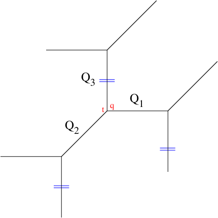
Figure 7: The ”toric” diagram of XHX_{H}. There are two choices for the preferred direction required by the refined vertex: The internal (1,1)(1,1) line or the two vertical external lines.

This geometry XHX_{H} can also be obtained by partial compactfication of X0X_{0} [15]. In terms of toric diagrams this corresponds to a non-planar toric diagram obtained from the toric diagram of X0X_{0} by gluing two of the parallel external edges. This gives rise to another ℙ1\mathbb{P}^{1} in the geometry such that the new Kähler parameter is proportional to the mass mm of the adjoint hypermultiplet. This is shown in Fig. 7. In this case the refined vertex calculation can be done in two different ways corresponding to two different choices for the preferred direction: The internal (1,1)(1,1) line or the two vertical external edges.

3.2 Refined partition function

We begin with the calculation of the refined partition function of this theory using the refined topological vertex formalism [9] and the toric diagram of XHX_{H} given above. Recall that the refined vertex calculation requires a preferred direction at each vertex such that all preferred directions of a given toric diagram be parallel33 3 For an arbitrary toric diagram this may not be possible. An example is the toric diagram of 𝒪⁡(−3)↦ℙ2{\cal O}(-3)\mapsto\mathbb{P}^{2}. This condition is actually equivalent to requiring that the corresponding CY3-fold be such that it gives rise to a supersymmetric gauge theory via geometric engineering. Thus this CY will be some AnA_{n} fibration over a chain of ℙ1\mathbb{P}^{1}’s. The preferred direction then corresponds to the base of this fibration.. In the case of XHX_{H} we see that there are two choices for the preferred direction corresponding to two seemingly different partition functions. Choosing the preferred direction to be the vertical external legs we get:

Z(1)​(Q,Qm,t,q)\displaystyle Z^{(1)}(Q,Q_{m},t,q) =\displaystyle= ∑λ,μ(−Qm)|μ|​(−Q)|λ|​Cλ​μ​∅​(t,q)​Cλt​μt​∅​(q,t)\displaystyle\sum_{\lambda,\mu}(-Q_{m})^{|\mu|}(-Q)^{|\lambda|}C_{\lambda\mu\emptyset}(t,q)C_{\lambda^{t}\mu^{t}\emptyset}(q,t) (3.1)
=\displaystyle= ∑λ,μ,η1,η2(−Qm)|μ|​(−Q)|λ|​(qt)|η1|−|η2|2​sλt/η1​(t−ρ)​sμ/η1​(q−ρ)​sλ/η2​(q−ρ)​sμt/η2​(t−ρ)\displaystyle\sum_{\lambda,\mu,\eta_{1},\eta_{2}}(-Q_{m})^{|\mu|}(-Q)^{|\lambda|}\left(\frac{q}{t}\right)^{\frac{|\eta_{1}|-|\eta_{2}|}{2}}s_{\lambda^{t}/\eta_{1}}(t^{-\rho})s_{\mu/\eta_{1}}(q^{-\rho})s_{\lambda/\eta_{2}}(q^{-\rho})s_{\mu^{t}/\eta_{2}}(t^{-\rho})
=\displaystyle= M​(t,q)−1​∑λ,μQ∙|λ|​sλ/μ​(t−ρ+12​q−12,Q−1​tρ)​sλ/μ​(q−ρ,qt​Qm−1​qρ)\displaystyle M(t,q)^{-1}\sum_{\lambda,\mu}Q_{\bullet}^{|\lambda|}\,s_{\lambda/\mu}\Big(t^{-\rho+\frac{1}{2}}q^{-\frac{1}{2}},Q^{-1}t^{\rho}\Big)s_{\lambda/\mu}\Big(q^{-\rho},\sqrt{\frac{q}{t}}Q_{m}^{-1}\,q^{\rho}\Big)
=\displaystyle= ∏i,j=1∞(1−Qm​qi−12​tj−12)​Z^(1)​(Q,Qm,t,q)\displaystyle\prod_{i,j=1}^{\infty}(1-Q_{m}\,q^{i-\frac{1}{2}}\,t^{j-\frac{1}{2}})\,\widehat{Z}^{(1)}(Q,Q_{m},t,q)

where

Q\displaystyle Q =\displaystyle= e−T,Qm=e−Tm,T,Tm​are the two Kähler parameters\displaystyle e^{-T}\,,\,\,Q_{m}=e^{-T_{m}}\,,\,\,T,T_{m}\,\,\,\mbox{are the two K\"{a}hler parameters}
M⁡(t,q)\displaystyle M(t,q) =\displaystyle= ∏i,j=1∞(1−ti−1​qj)−1,Q∙=Q​Qm\displaystyle\prod_{i,j=1}^{\infty}(1-t^{i-1}\,q^{j})^{-1}\,,\,\,\,\,\,\,\,\,\,Q_{\bullet}=Q\,Q_{m}
Z^(1)​(Q,Qm,t,q)\displaystyle\ \widehat{Z}^{(1)}(Q,Q_{m},t,q) =\displaystyle= ∑λ,μQ|λ|​Qm|μ|​sλ/μ​(−Qm(1)​qt​qρ,q−ρ)​sλt/μt​(Qm(2)​tq​tρ,t−ρ)\displaystyle\sum_{\lambda,\mu}Q^{|\lambda|}\,Q_{m}^{|\mu|}s_{\lambda/\mu}\Big(-Q_{m}^{(1)}\sqrt{\frac{q}{t}}\,q^{\rho},q^{-\rho}\Big)s_{\lambda^{t}/\mu^{t}}\Big(Q_{m}^{(2)}\sqrt{\frac{t}{q}}\,t^{\rho},t^{-\rho}\Big) (3.2)

On the other hand choosing the internal (1,1)(1,1) leg to be the preferred direction we get:

Z(2)​(Q,Qm,t,q)\displaystyle Z^{(2)}(Q,Q_{m},t,q) =\displaystyle= ∑λ,ν(−Q)|ν|​(−Qm)|λ|​C∅​λ​ν​(t,q)​C∅​λt​νt​(q,t)\displaystyle\sum_{\lambda,\nu}(-Q)^{|\nu|}(-Q_{m})^{|\lambda|}C_{\emptyset\lambda\nu}(t,q)C_{\emptyset\lambda^{t}\nu^{t}}(q,t) (3.3)
=\displaystyle= ∑ν(−Q)|ν|​q‖ν‖22​t‖νt‖22​Z~ν​(t,q)​Z~νt​(q,t)​∏i,j=1∞(1−Qm​q−μi−ρj​t−μjt−ρi)\displaystyle\sum_{\nu}(-Q)^{|\nu|}q^{\frac{||\nu||^{2}}{2}}\,t^{\frac{||\nu^{t}||^{2}}{2}}\widetilde{Z}_{\nu}(t,q)\,\widetilde{Z}_{\nu^{t}}(q,t)\prod_{i,j=1}^{\infty}(1-Q_{m}\,q^{-\mu_{i}-\rho_{j}}t^{-\mu^{t}_{j}-\rho_{i}})
=\displaystyle= ∏i,j=1+∞(1−Qm​ti−12​qj−12)​Z^(2)​(Q,Qm,t,q),\displaystyle\prod_{i,j=1}^{+\infty}(1-Q_{m}\,t^{i-\frac{1}{2}}\,q^{j-\frac{1}{2}})\,\widehat{Z}^{(2)}(Q,Q_{m},t,q)\,,

where

Z^(2)​(Q,Qm,t,q)=∑ν(Q​Qm)|ν|​∏s∈ν(1−Qm​ta⁡(s)+12​qℓ⁡(s)+12)​(1−Qm−1​qℓ⁡(s)+12​ta⁡(s)+12)(1−ta⁡(s)+1​qℓ⁡(s))​(1−qℓ⁡(s)+1​ta⁡(s)).\displaystyle\widehat{Z}^{(2)}(Q,Q_{m},t,q)=\sum_{\nu}(QQ_{m})^{|\nu|}\prod_{s\in\nu}\frac{(1-Q_{m}\,t^{a(s)+\frac{1}{2}}\,q^{\ell(s)+\frac{1}{2}})(1-Q_{m}^{-1}\,q^{\ell(s)+\frac{1}{2}}\,t^{a(s)+\frac{1}{2}})}{(1-t^{a(s)+1}\,q^{\ell(s)})(1-q^{\ell(s)+1}\,t^{a(s)})}\,. (3.4)

Note that:
■\blacksquare In Eq.(3.2) we have introduced superscripts on Qm(1)Q_{m}^{(1)} and Qm(2)Q_{m}^{(2)} just to distinguish the arguments of the skew-Schur function from each other. But we will always take Qm(1)=Qm(2)=QmQ_{m}^{(1)}=Q_{m}^{(2)}=Q_{m}.
■\blacksquare In going from Eq. (3.3) to Eq. (3.4) we have used the following identity [Nakajima:2003pg]:

∏i,j=1∞(1−Qm​q−νi−ρj​t−νjt−ρi)∏i,j=1∞(1−Qm​q−ρi​t−ρj)=∏s∈ν(1−Qm​q−ℓ⁡(s)−12​t−a⁡(s)−12)​(1−Qm​qℓ⁡(s)+12​ta⁡(s)+12)\displaystyle\frac{\prod_{i,j=1}^{\infty}\left(1-Q_{m}\,q^{-\nu_{i}-\rho_{j}}\,t^{-\nu_{j}^{t}-\rho_{i}}\right)}{\prod_{i,j=1}^{\infty}\left(1-Q_{m}\,q^{-\rho_{i}}\,t^{-\rho_{j}}\right)}=\prod_{s\in\nu}\left(1-Q_{m}\,q^{-\ell(s)-\frac{1}{2}}\,t^{-a(s)-\frac{1}{2}}\right)\left(1-Q_{m}\,q^{\ell(s)+\frac{1}{2}}\,t^{a(s)+\frac{1}{2}}\right)

The two expressions Z(1)​(Q,Qm,t,q)Z^{(1)}(Q,Q_{m},t,q) and Z(2)​(Q,Qm,t,q)Z^{(2)}(Q,Q_{m},t,q) (and therefore Z^(1)​(Q,Qm,t,q)\widehat{Z}^{(1)}(Q,Q_{m},t,q) and Z^(2)​(Q,Qm,t,q)\widehat{Z}^{(2)}(Q,Q_{m},t,q)) appear different but are actually equal to each other as can be seen by expanding them in powers of QQ and QmQ_{m} therefore from now on we will not use the superscript to distinguish them unless we need a specific form of the partition function. Thus we see that different choices for the preferred direction for a given toric diagram give rise to non-trivial (q,t)(q,t) identities involving “principal specialization” of the Macdonald function [17]. In section 4 we will give some other examples of (q,t)(q,t) identities arising from the refined topological vertex calculation.

In the gauge theory language Z^(1)​(Q,Qm,t,q)\widehat{Z}^{(1)}(Q,Q_{m},t,q) or Z^(2)​(Q,Qm,t,q)\widehat{Z}^{(2)}(Q,Q_{m},t,q) is the contribution to the gauge theory partition function coming from instantons whereas the prefactor ∏i,j(1−Qm​ti−12​qj−12)\prod_{i,j}(1-Q_{m}t^{i-\frac{1}{2}}\,q^{j-\frac{1}{2}}) is the perturbative contribution. For the moment we will ignore this prefactor and focus only on the instanton contribution. The partition function Z⁡(Q,Qm,t,q)Z(Q,Q_{m},t,q) is invariant under the exchange of QQ and QmQ_{m} but Z^​(Q,Qm,t,q)\widehat{Z}(Q,Q_{m},t,q) is not invariant under this exchange.

Using the identity

∑λ,μQ∙|λ|​sλ/μ​(𝐱)​sλ/μ​(𝐲)=∏k=1∞((1−Q∙k)−1​∏i,j=1∞(1−Q∙k​xi​yj)−1),\displaystyle\sum_{\lambda,\mu}Q_{\bullet}^{|\lambda|}\,s_{\lambda/\mu}({\bf x})\,s_{\lambda/\mu}({\bf y})=\prod_{k=1}^{\infty}\Big((1-Q_{\bullet}^{k})^{-1}\,\prod_{i,j=1}^{\infty}(1-Q_{\bullet}^{k}x_{i}y_{j})^{-1}\Big)\,, (3.5)

we can write Z⁡(Q,Qm,t,q)Z(Q,Q_{m},t,q) in Eq.(3.1) in a product form:

Z⁡(Q,Qm,t,q)=M​(t,q)−1​∏k=1∞((1−Q∙k)​∏i,j=1∞(1−Q∙k​Qm−1​q−i+12​tj−12)​(1−Q∙k​Q−1​qi−12​t−j+12)CLOSE\displaystyle Z(Q,Q_{m},t,q)=M(t,q)^{-1}\prod_{k=1}^{\infty}\Big((1-Q_{\bullet}^{k})\prod_{i,j=1}^{\infty}(1-Q_{\bullet}^{k}Q_{m}^{-1}q^{-i+\frac{1}{2}}t^{j-\frac{1}{2}})(1-Q_{\bullet}^{k}Q^{-1}q^{i-\frac{1}{2}}t^{-j+\frac{1}{2}})
×(1−Q∙kqi−1tj)(1−Q∙k−1q−i+1t−j))−1.\displaystyle\times(1-Q_{\bullet}^{k}\,q^{i-1}t^{j})(1-Q_{\bullet}^{k-1}\,q^{-i+1}t^{-j})\Big)^{-1}.

If |t|<1|t|<1 and |q|<1|q|<1 (i.e., ϵ1​<0,ϵ2>​0\epsilon_{1}<0,\epsilon_{2}>0) then we should write the above as

Z⁡(Q,Qm,t,q)=∏k=1∞((1−Q∙k)−1​∏i,j=1∞(1−Q∙k​Qm−1​qi−12​tj−12)​(1−Q∙k​Q−1​qi−12​tj−12)(1−Q∙k​qi−1​tj)​(1−Q∙k​qi​tj−1)).\displaystyle Z(Q,Q_{m},t,q)=\prod_{k=1}^{\infty}\Big((1-Q_{\bullet}^{k})^{-1}\prod_{i,j=1}^{\infty}\frac{(1-Q_{\bullet}^{k}\,Q_{m}^{-1}\,q^{i-\frac{1}{2}}\,t^{j-\frac{1}{2}})(1-Q_{\bullet}^{k}\,Q^{-1}\,q^{i-\frac{1}{2}}t^{j-\frac{1}{2}})}{(1-Q_{\bullet}^{k}\,q^{i-1}t^{j})(1-Q_{\bullet}^{k}\,q^{i}t^{j-1})}\Big)\,.

On the other hand if |t|>1|t|>1 and |q|<1|q|<1 (i.e., ϵ1>0,ϵ2>0\epsilon_{1}>0,\epsilon_{2}>0) then we should write the above partition function in terms of qq and t−1t^{-1} so that

Z⁡(Q,Qm,t,q)=∏k=1∞((1−Q∙k)−1​∏i,j(1−Q∙k​qi−1​t1−j)​(1−Q∙k​qi​t−j)(1−Q∙k​Qm−1​qi−12​t−j+12)​(1−Q∙k​Q−1​qi−12​t−j+12)).\displaystyle Z(Q,Q_{m},t,q)=\prod_{k=1}^{\infty}\Big((1-Q_{\bullet}^{k})^{-1}\prod_{i,j}\frac{(1-Q_{\bullet}^{k}\,q^{i-1}t^{1-j})(1-Q_{\bullet}^{k}\,q^{i}t^{-j})}{(1-Q_{\bullet}^{k}Q_{m}^{-1}q^{i-\frac{1}{2}}\,t^{-j+\frac{1}{2}})(1-Q_{\bullet}^{k}Q^{-1}q^{i-\frac{1}{2}}t^{-j+\frac{1}{2}})}\Big)\,.

3.3 Field theory limit

If we denote the mass of the adjoint by mm then the 4D field theory limit is given by44 4 In identifying QmQ_{m} with the mass mm we have introduced a factor of tq\sqrt{\frac{t}{q}} so that the m↦0m\mapsto 0 limit gives the partition function of 𝒩=4{\mathcal{N}}=4 gauge theory. For the discussion of the relation between (q,t)(q,t) and the Ω\Omega-background [8] parameters (ϵ1,ϵ2)(\epsilon_{1},\epsilon_{2}) we refer the reader to [9].

Qm=tq​e−β​m,t=eβ​ϵ1,q=e−β​ϵ2,β↦0.\displaystyle Q_{m}=\sqrt{\frac{t}{q}}\,e^{-\beta m}\,,\,\,t=e^{\,\beta\epsilon_{1}}\,,q=e^{-\,\beta\epsilon_{2}}\,,\,\,\beta\mapsto 0\,. (3.6)

We will see that the two instanton partition functions Z^(1)​(Q,Qm,t,q)\widehat{Z}^{(1)}(Q,Q_{m},t,q) and Z^(2)​(Q,Qm,t,q)\widehat{Z}^{(2)}(Q,Q_{m},t,q) give rise to an interesting identity in the above limit. We begin with Z^(2)​(Q,Qm,t,q)\widehat{Z}^{(2)}(Q,Q_{m},t,q) as it is easy to see what the field theory limit of this is:

Z^(2)​(Q,Qm,t,q)↦β↦0\displaystyle\widehat{Z}^{(2)}(Q,Q_{m},t,q)\xmapsto{\beta\mapsto 0} 𝒵^​(Q,m,ϵ1,ϵ2)\displaystyle\widehat{{\cal Z}}(Q,m,\epsilon_{1},\epsilon_{2})
=\displaystyle= ∑νQ|ν|​∏s∈ν(a⁡(s)+1+ϑ​ℓ​(s)−m~)​(a⁡(s)+ϑ⁡(ℓ⁡(s)+1)+m~)(a⁡(s)+1+ϑ​ℓ​(s))​(a⁡(s)+ϑ⁡(ℓ⁡(s)+1)),\displaystyle\sum_{\nu}Q^{|\nu|}\prod_{s\in\nu}\frac{(a(s)+1+\vartheta\,\ell(s)-\widetilde{m})(a(s)+\vartheta\,(\ell(s)+1)+\widetilde{m})}{(a(s)+1+\vartheta\,\ell(s))(a(s)+\vartheta(\ell(s)+1))},

where ϑ=−ϵ2/ϵ1\vartheta=-\epsilon_{2}/\epsilon_{1} and m~=m/ϵ1\widetilde{m}=m/\epsilon_{1}. The product inside the sum, in the expression above, gives a generalization of Nekrasov-Okounkov probability measure [18] on the set of partitions [19] 55 5 h⁡(i,j)=a⁡(i,j)+ℓ⁡(i,j)+1h(i,j)=a(i,j)+\ell(i,j)+1 is the hook length.,

∏s∈λh​(s)2−m~2h​(s)2↦∏s∈λ(a⁡(s)+1+ϑ​ℓ​(s)−m~)​(a⁡(s)+ϑ​ℓ​(s)+ϑ+m~)OPEN(a⁡(s)+1+ϑ​ℓ​(s))​(a⁡(s)+ϑ​ℓ​(s)+ϑ))\displaystyle\prod_{s\in\lambda}\frac{h(s)^{2}-\widetilde{m}^{2}}{h(s)^{2}}\mapsto\prod_{s\in\lambda}\frac{\Big(a(s)+1+\vartheta\,\ell(s)-\widetilde{m}\Big)\Big(a(s)+\vartheta\,\ell(s)+\vartheta+\widetilde{m}\Big)}{\Big(a(s)+1+\vartheta\,\ell(s)\Big)\Big(a(s)+\vartheta\,\ell(s)+\vartheta)\Big)} (3.7)
↦∏s∈λ(1−Qm​ta⁡(s)+1​qℓ⁡(s))​(1−Qm−1​qℓ⁡(s)+1​ta⁡(s))(1−ta⁡(s)+1​qℓ⁡(s))​(1−qℓ⁡(s)+1​ta⁡(s))\displaystyle\mapsto\prod_{s\in\lambda}\frac{(1-Q_{m}\,t^{a(s)+1}\,q^{\ell(s)})(1-Q_{m}^{-1}\,q^{\ell(s)+1}\,t^{a(s)})}{(1-t^{a(s)+1}\,q^{\ell(s)})(1-q^{\ell(s)+1}\,t^{a(s)})}

It was shown in [18] that for ϑ=1\vartheta=1 (ϵ1+ϵ2=0\epsilon_{1}+\epsilon_{2}=0),

𝒵^​(Q,m,ϵ1,−ϵ1)=∏n=1∞(1−Qn)m~2−1.\displaystyle\widehat{{\cal Z}}(Q,m,\epsilon_{1},-\epsilon_{1})=\prod_{n=1}^{\infty}\Big(1-Q^{n}\Big)^{\widetilde{m}^{2}-1}. (3.8)

Taking the field theory limit of Z^(1)​(Q,Qm,t,q)\widehat{Z}^{(1)}(Q,Q_{m},t,q) in Eq.(3.2) is slightly more subtle. To take this limit first notice that the argument of the first skew-Schur function in Eq.(3.2) is an infinite set which reduces to a finite set if we take Qm(1)=tq​qMQ^{(1)}_{m}=\sqrt{\frac{t}{q}}\,q^{M} and analytically continue to |q|<1|q|<1. The same is true for the argument of the second skew-Schur function:

{Qm(1)​qt​qρ,q−ρ}↦Qm(1)=tq​qM\displaystyle\{Q_{m}^{(1)}\sqrt{\frac{q}{t}}\,q^{\rho},q^{-\rho}\}\,\xmapsto{Q^{(1)}_{m}=\sqrt{\frac{t}{q}}\,q^{M}} =\displaystyle= {q12,q32,q52,⋯,qM−12}\displaystyle\{q^{\frac{1}{2}},q^{\frac{3}{2}},q^{\frac{5}{2}},\cdots,q^{M-\frac{1}{2}}\} (3.9)
{Qm(2)​tq​tρ,t−ρ}↦Qm(2)=qt​tL\displaystyle\{Q_{m}^{(2)}\sqrt{\frac{t}{q}}\,t^{\rho},t^{-\rho}\}\,\xmapsto{Q^{(2)}_{m}=\sqrt{\frac{q}{t}}\,t^{L}} =\displaystyle= {t12,t32,t52,⋯,tL−12}\displaystyle\{t^{\frac{1}{2}},t^{\frac{3}{2}},t^{\frac{5}{2}},\cdots,t^{L-\frac{1}{2}}\}

With this identification Eq. (3.2) gives

Z^(1)​(Q,Qm,t,q)\displaystyle\widehat{Z}^{(1)}(Q,Q_{m},t,q) =\displaystyle= ∑λ,μ(−Q)|λ|​(−Qm)|μ|​sλ/μ​(q12,q32,q52,⋯,qM−12)​sλt/μt​(t12,t32,⋯,tL−12)\displaystyle\sum_{\lambda,\mu}(-Q)^{|\lambda|}\,(-Q_{m})^{|\mu|}s_{\lambda/\mu}(q^{\frac{1}{2}},q^{\frac{3}{2}},q^{\frac{5}{2}},\cdots,q^{M-\frac{1}{2}})\,s_{\lambda^{t}/\mu^{t}}(t^{\frac{1}{2}},t^{\frac{3}{2}},\cdots,t^{L-\frac{1}{2}})
=\displaystyle= ∏k=1∞((1−Qk​Qmk)−1​∏i,j=1M,L(1−Qk​Qmk−1​qi−12​tj−12)).\displaystyle\prod_{k=1}^{\infty}\Big((1-Q^{k}Q_{m}^{k})^{-1}\,\prod_{i,j=1}^{M,L}(1-Q^{k}Q_{m}^{k-1}\,q^{i-\frac{1}{2}}\,t^{j-\frac{1}{2}})\Big).

In the field theory limit given by Eq. (3.6) we get

Z^(1)​(Q,Qm,t,q)↦β↦0𝒵^​(Q,m,ϵ1,ϵ2)=∏k=1∞(1−Qk)M​L−1.\displaystyle\widehat{Z}^{(1)}(Q,Q_{m},t,q)\xmapsto{\beta\mapsto 0}\widehat{\cal Z}(Q,m,\epsilon_{1},\epsilon_{2})=\prod_{k=1}^{\infty}(1-Q^{k})^{ML-1}\,. (3.10)

But since Qm(1)=Qm(2)=tq​e−β​mQ_{m}^{(1)}=Q_{m}^{(2)}=\sqrt{\frac{t}{q}}\,e^{-\beta m},

tq​qM\displaystyle\sqrt{\frac{t}{q}}\,q^{M} =\displaystyle= qt​tL⇒ϵ1​(L−1)=−ϵ2​(M−1)⇒L−1=ϑ⁡(M−1),\displaystyle\sqrt{\frac{q}{t}}\,t^{L}\,\Rightarrow\,\epsilon_{1}(L-1)=-\epsilon_{2}(M-1)\Rightarrow L-1=\vartheta(M-1)\,, (3.11)
m\displaystyle m =\displaystyle= ϵ2​M,.\displaystyle\epsilon_{2}\,M,\,.

which implies that

M​L−1\displaystyle ML-1 =\displaystyle= (M−1)​(ϑ​M+1)\displaystyle(M-1)(\vartheta\,M+1) (3.12)
=\displaystyle= −(m−ϵ1)​(m−ϵ2)ϵ1​ϵ2.\displaystyle-\frac{(m-\epsilon_{1})(m-\epsilon_{2})}{\epsilon_{1}\,\epsilon_{2}}\,\,.

Thus we see that in the field theory limit

Z^​(Q,Qm,t,q)↦β↦0𝒵^​(Q,m,ϵ1,ϵ2)=∏k=1∞(1−Qk)−(m−ϵ1)​(m−ϵ2)ϵ1​ϵ2.\displaystyle\widehat{Z}(Q,Q_{m},t,q)\xmapsto{\beta\mapsto 0}\widehat{\cal Z}(Q,m,\epsilon_{1},\epsilon_{2})=\prod_{k=1}^{\infty}(1-Q^{k})^{-\frac{(m-\epsilon_{1})(m-\epsilon_{2})}{\epsilon_{1}\,\epsilon_{2}}}. (3.13)

This gives us the following interesting identity:

∑νQ|ν|​∏s∈ν(a⁡(s)+1+ϑ​ℓ​(s)−m~)​(a⁡(s)+ϑ⁡(ℓ⁡(s)+1)+m~)(a⁡(s)+1+ϑ​ℓ​(s))​(a⁡(s)+ϑ⁡(ℓ⁡(s)+1))=∏k=1∞(1−Qk)(m~−1)​(m~+ϑ)ϑ\sum_{\nu}Q^{|\nu|}\prod_{s\in\nu}\frac{(a(s)+1+\vartheta\,\ell(s)-\tilde{m})(a(s)+\vartheta\,(\ell(s)+1)+\tilde{m})}{(a(s)+1+\vartheta\,\ell(s))(a(s)+\vartheta(\ell(s)+1))}=\prod_{k=1}^{\infty}(1-Q^{k})^{\frac{(\tilde{m}-1)(\tilde{m}+\vartheta)}{\vartheta}}

4 Periodic Schur Process

Let us denote by P the set of Young diagrams. A periodic Schur process is a random process defined on P2​K\textsf{P}^{2K} such that it assigns to a set {λ(a),μ(a+1)|a=0,1⋯,K−1}\{\lambda^{(a)},\mu^{(a+1)}\,|\,a=0,1\cdots,K-1\} of 2​K2K partitions the weight [3]

1GK×φ|λ(0)|∏a=0K−1sλ(a)/μ(a+1)(𝐱a+1)sλ(a+1)/μ(a+1)(𝐲a+1)\displaystyle\frac{1}{G_{K}}\times\varphi^{|\lambda^{(0)}|}\,\prod_{a=0}^{K-1}s_{\lambda^{(a)}/\mu^{(a+1)}}({\bf x}_{a+1})s_{\lambda^{(a+1)}/\mu^{(a+1)}}({\bf y}_{a+1}) (4.1)

where λ(K)=λ(0)\lambda^{(K)}=\lambda^{(0)}, 𝐱a,𝐲a{\bf x}_{a},{\bf y}_{a} are specializations of the algebra of symmetric functions and GKG_{K} is the partition function of the process,

GK​(φ,𝐱,𝐲):=∑λ(0)​μ(1),⋯,λ(K−1),μ(K)φ|λ(0)|​∏a=0K−1sλ(a)/μ(a+1)​(𝐱a+1)​sλ(a+1)/μ(a+1)​(𝐲a+1).\displaystyle G_{K}(\varphi,{\bf x},{\bf y}):=\sum_{\lambda^{(0)}\mu^{(1)},\cdots,\lambda^{(K-1)},\mu^{(K)}}\varphi^{|\lambda^{(0)}|}\,\prod_{a=0}^{K-1}s_{\lambda^{(a)}/\mu^{(a+1)}}({\bf x}_{a+1})s_{\lambda^{(a+1)}/\mu^{(a+1)}}({\bf y}_{a+1})\,. (4.2)

We will consider the case when K=1K=1 which is closely related, as we will see, to the counting of cylindric plane partitions. For K=1K=1 the weight assigned to the pair {λ,μ}\{\lambda,\mu\} is

1G1×sλ/μ​(𝐱)​sλ/μ​(𝐲)\displaystyle\frac{1}{G_{1}}\times s_{\lambda/\mu}({\bf x})\,s_{\lambda/\mu}({\bf y}) (4.3)

and

G1​(φ,𝐱,𝐲)=∑λ,μφ|λ|​sλ/μ​(𝐱)​sλ/μ​(𝐲).\displaystyle G_{1}(\varphi,{\bf x},{\bf y})=\sum_{\lambda,\mu}\varphi^{|\lambda|}\,s_{\lambda/\mu}({\bf x})\,s_{\lambda/\mu}({\bf y})\,. (4.4)

If we take a particular specialization

𝐱\displaystyle{\bf x} =\displaystyle= 𝐱⁡(t,q,Q)={t−ρ+12​q−12,Q−1​tρ}\displaystyle{\bf x}(t,q,Q)=\{t^{-\rho+\frac{1}{2}}\,q^{-\frac{1}{2}},Q^{-1}t^{\rho}\} (4.5)
𝐲\displaystyle{\bf y} =\displaystyle= 𝐲⁡(t,q,Qm)={q−ρ,qt​Qm−1​qρ},\displaystyle{\bf y}(t,q,Q_{m})=\{q^{-\rho},\sqrt{\frac{q}{t}}\,Q_{m}^{-1}\,q^{\rho}\}\,, (4.6)

and take φ=Q∙\varphi=Q_{\bullet} then from Eq(3.1) it follows that

G1​(Q∙,𝐱⁡(t,q,Q),𝐲⁡(t,q,Qm))=M⁡(t,q)​Z(1)​(Q,Qm,t,q)\displaystyle G_{1}(Q_{\bullet},{\bf x}(t,q,Q),{\bf y}(t,q,Q_{m}))=M(t,q)\,Z^{(1)}(Q,Q_{m},t,q) (4.7)

Thus the partition function of the K=1K=1 periodic Schur process is precisely the partition function of the abelian gauge theory with an adjoint hypermultiplet. It was shown in [3] that the K=1K=1 Schur process is related to the counting of cylindric partitions. The cylindric partitions, first introduced in [20], are generalizations of the plane partitions. However, for our purposes, the reparameterization of them in [3] is more suitable, which we largely follow.

A cylindric plane partition of type (n,ℓ)(n,\ell) is an infinite array {πi,j|i,j∈ℤ}\{\pi_{i,j}\,|\,i,j\in\mathbb{Z}\} of non-negative numbers such that:

πi,j​is weakly decreasing in both i and j,\displaystyle\pi_{i,j}\,\mbox{is weakly decreasing in both $i$ and $j$}\,,
πi,j=πi+n,j−ℓ.\displaystyle\pi_{i,j}=\pi_{i+n,j-\ell}\,.

The figure below shows an example of a cylindric partition. It is an infinite periodic diagram with one period shown between the vertical lines. Since the partitions on the vertical lines are identical we can glue them together and instead consider a finite diagram on a cylinder with period n+ℓn+\ell.

Refer to caption
Figure 8: An example for a cylindric partition with (n,ℓ)=(4,10)(n,\ell)=(4,10).

Let us define 𝔾n,ℓ​(s)\mathbb{G}^{n,\ell}(s) to be the generating function of cylindric plane partitions of type (n,ℓ)(n,\ell),

𝔾n,ℓ​(s)=∑cylindric partitions π of type (n,ℓ)s|π|,\displaystyle\mathbb{G}^{n,\ell}(s)=\sum_{\mbox{\tiny cylindric partitions $\pi$ of type $(n,\ell)$}}\,s^{|\pi|}\,, (4.8)

where |π|=∑i=1,j=1n,ℓπi,j|\pi|=\sum_{i=1,j=1}^{n,\ell}\pi_{i,j}. This generating function was determined in [3] and is given by

𝔾n,ℓ​(s)=∏k=1∞((1−sk⁡(n+ℓ))−1​∏i=1,j=1ℓ,n(1−sk⁡(n+ℓ)−i−j+1)−1).\displaystyle\mathbb{G}^{n,\ell}(s)=\prod_{k=1}^{\infty}\Big((1-s^{k\,(n+\ell)})^{-1}\prod_{i=1,j=1}^{\ell,n}(1-s^{k\,(n+\ell)-i-j+1})^{-1}\Big)\,. (4.9)

We will show that this generating function is exactly the partition function of XHX_{H} after an identification of parameters. To see this recall that the partition function of XHX_{H} (Eq(3.1)) is given by

Z(1)​(Q,Qm,t,q)\displaystyle Z^{(1)}(Q,Q_{m},t,q) =\displaystyle= M​(t,q)−1​ℤ​(Q,Qm,t,q)\displaystyle M(t,q)^{-1}\,\mathbb{Z}(Q,Q_{m},t,q) (4.10)
ℤ⁡(Q,Qm,t,q)\displaystyle\mathbb{Z}(Q,Q_{m},t,q) =\displaystyle= ∑λ,μQ∙|λ|​sλ/μ​(t−ρ​tq,Q−1​tρ)​sλ/μ​(q−ρ,qt​Qm−1​qρ)\displaystyle\sum_{\lambda,\mu}Q_{\bullet}^{|\lambda|}\,s_{\lambda/\mu}\Big(t^{-\rho}\sqrt{\frac{t}{q}},Q^{-1}t^{\rho}\Big)s_{\lambda/\mu}\Big(q^{-\rho},\sqrt{\frac{q}{t}}Q_{m}^{-1}\,q^{\rho}\Big)\,

The arguments of the two skew-Schur functions in the above equation are an infinite set of variables. By quantizing the two Kähler parameters (and analytic continuation to |q|<1,|t|<1|q|<1,|t|<1) we can convert these infinite set of variables into a finite set:

{tiq−12,Q−1t−i+12|i≥1}\displaystyle\{t^{i}q^{-\frac{1}{2}},Q^{-1}t^{-i+\frac{1}{2}}\,|\,i\geq 1\} ↦Q=qt​t−ℓ{tiq−12|i=1,2,⋯,ℓ}\displaystyle\xmapsto{Q=\sqrt{\frac{q}{t}}\,t^{-\ell}}\,\,\,\{t^{i}\,q^{-\frac{1}{2}}\,|\,i=1,2,\cdots,\ell\} (4.11)
{qi−12,qtQm−1q−i+12|i≥1}\displaystyle\{q^{i-\frac{1}{2}},\sqrt{\frac{q}{t}}Q_{m}^{-1}\,q^{-i+\frac{1}{2}}\,|\,i\geq 1\} ↦Qm=tq​q−n{qi−12|i=1,2,⋯,n}\displaystyle\xmapsto{Q_{m}=\sqrt{\frac{t}{q}}\,q^{-n}}\,\,\,\{q^{i-\frac{1}{2}}\,|\,i=1,2,\cdots,n\}

Eq(4.10) becomes

ℤ⁡(Q=qt​t−ℓ,Qm=tq​q−n,t,q)\displaystyle\mathbb{Z}\Big(Q=\sqrt{\frac{q}{t}}\,t^{-\ell},Q_{m}=\sqrt{\frac{t}{q}}\,q^{-n},t,q\Big) =\displaystyle= ∑λ,μ(t−ℓ​q−n)|λ|​sλ/μ​(t​q−12,t2​q−12,⋯,tℓ​q−12)\displaystyle\sum_{\lambda,\mu}(t^{-\ell}\,q^{-n})^{|\lambda|}\,s_{\lambda/\mu}\Big(t\,q^{-\frac{1}{2}},t^{2}\,q^{-\frac{1}{2}},\cdots,t^{\ell}\,q^{-\frac{1}{2}}\Big)
×\displaystyle\times sλ/μ​(q12,q32,⋯,qn−12)\displaystyle s_{\lambda/\mu}\Big(q^{\frac{1}{2}},q^{\frac{3}{2}},\cdots,q^{n-\frac{1}{2}}\Big)\,
=\displaystyle= ∏k=1∞((1−(t−ℓ​q−n)k)​∏i,j=1n,ℓ(1−qi−1−k​n​tj−k​ℓ)CLOSE\displaystyle\prod_{k=1}^{\infty}\Big((1-(t^{-\ell}\,q^{-n})^{k})\prod_{i,j=1}^{n,\ell}(1-q^{i-1-k\,n}\,t^{j-k\,\ell})

Comparing the above with Eq(4.9) we get

ℤ⁡(Q=sℓ,Qm=sn,s−1,s−1)=𝔾n,ℓ​(s)\mathbb{Z}\Big(Q=s^{\ell},Q_{m}=s^{n},s^{-1},s^{-1}\Big)\,=\,\mathbb{G}^{n,\ell}(s)\, (4.12)

The two Kähler parameters T,TmT,T_{m} are quantized and given by the positive integers (n,ℓ)(n,\ell) which define the type of the cylindric partitions:

T\displaystyle T =\displaystyle= ϵ1​ℓ+ϵ1+ϵ22\displaystyle\epsilon_{1}\,\ell+\frac{\epsilon_{1}+\epsilon_{2}}{2}
Tm\displaystyle T_{m} =\displaystyle= −ϵ2​n−ϵ1+ϵ22\displaystyle-\epsilon_{2}\,n-\frac{\epsilon_{1}+\epsilon_{2}}{2}

5 Hilbert schemes and Vertex Operators

The Hilbert schemes of ℂ2\mathbb{C}^{2} (OPENHilb∙​[ℂ2])\mbox{Hilb}^{\bullet}[\mathbb{C}^{2}]) play a central role in the Nekrasov’s derivation of the gauge theory partition functions using localization[8]. In this section we see that the topological string partition function of XHX_{H} can be written in terms of certain vertex operators which are generalization of operators related with the cohomology of the Hilbert scheme Hilb∙​[ℂ2]\mbox{Hilb}^{\bullet}[\mathbb{C}^{2}] and were studied recently in [5].

Recall that the instanton part of the gauge theory partition function of is given by Eq(3.2),

Z^(1)​(Q,Qm,t,q)\displaystyle\widehat{Z}^{(1)}(Q,Q_{m},t,q) =\displaystyle= ∑λ,μQ|λ|​Qm|μ|​sλ/μ​(−Qm​qt​qρ,q−ρ)​sλt/μt​(Qm​tq​tρ,t−ρ)\displaystyle\sum_{\lambda,\mu}Q^{|\lambda|}\,Q_{m}^{|\mu|}\,s_{\lambda/\mu}\Big(-Q_{m}\sqrt{\frac{q}{t}}\,q^{\rho},q^{-\rho}\Big)s_{\lambda^{t}/\mu^{t}}\Big(Q_{m}\sqrt{\frac{t}{q}}\,t^{\rho},\,t^{-\rho}\Big) (5.1)
=\displaystyle= ∑λ,μQ∙λ​sλ/μ​(Qm​qt​qρ,q−ρ)​sλ/μ​(Qm−1​tρ,tq​t−ρ)\displaystyle\sum_{\lambda,\mu}Q_{\bullet}^{\lambda}\,s_{\lambda/\mu}\Big(Q_{m}\sqrt{\frac{q}{t}}\,q^{\rho},q^{-\rho}\Big)s_{\lambda/\mu}\Big(Q_{m}^{-1}\,t^{\rho},\sqrt{\frac{t}{q}}\,t^{-\rho}\Big)

Where Q∙=Q​QmQ_{\bullet}=Q\,Q_{m} and in going from the first line in the above equation to the second line we have used the properties of the principal specialization of the Schur functions:

sλt/μt​(z​q−ρ,qρ)=(−z)|λ|−|μ|​sλ/μ​(z−1​q−ρ,qρ)\displaystyle s_{\lambda^{t}/\mu^{t}}(z\,q^{-\rho},q^{\rho})=(-z)^{|\lambda|-|\mu|}s_{\lambda/\mu}(z^{-1}q^{-\rho},q^{\rho}) (5.2)

The skew-Schur function in Eq(5.1) can be written as a matrix element of an operator. To see this note that

sλ/μ​(𝐱)=∑ηcη​μλ​sη​(𝐱),\displaystyle s_{\lambda/\mu}({\bf x})=\sum_{\eta}c^{\lambda}_{\eta\,\mu}\,s_{\eta}({\bf x})\,, (5.3)

where cη​μλc^{\lambda}_{\eta\,\mu} are the Littlewood-Richardson coefficients. Let us define an operator α~ν\widetilde{\alpha}_{\nu} labeled by a partition ν\nu such that

α~ν​|η⟩=∑λcν​ηλ​|λ⟩,\displaystyle\widetilde{\alpha}_{\nu}|\eta\rangle=\sum_{\lambda}c^{\lambda}_{\nu\,\eta}\,|\lambda\rangle\,, (5.4)

It follows from the above that

cν​ηλ=⟨λ|α~ν|η⟩=⟨η|α~ν†|λ⟩.\displaystyle c^{\lambda}_{\nu\,\eta}=\langle\lambda|\widetilde{\alpha}_{\nu}|\eta\rangle=\langle\eta|\widetilde{\alpha}_{\nu}^{\dagger}|\lambda\rangle\,. (5.5)

Then we see that the skew-Schur function can be written as

sλ/μ​(𝐱)\displaystyle s_{\lambda/\mu}({\bf x}) =\displaystyle= ∑ηcη​μλ​sη​(𝐱)=∑η⟨λ|α~η|μ⟩​sη​(𝐱)\displaystyle\sum_{\eta}c^{\lambda}_{\eta\,\mu}\,s_{\eta}({\bf x})=\sum_{\eta}\langle\lambda|\widetilde{\alpha}_{\eta}|\mu\rangle\,s_{\eta}({\bf x}) (5.6)
=\displaystyle= ⟨λ|(∑ηsη​(𝐱)​α~η)|μ⟩=⟨μ|(∑ηsη​(𝐱)​α~η†)|λ⟩.\displaystyle\langle\lambda|\Big(\sum_{\eta}\,s_{\eta}({\bf x})\widetilde{\alpha}_{\eta}\Big)|\mu\rangle\,=\langle\mu|\Big(\sum_{\eta}\,s_{\eta}({\bf x})\widetilde{\alpha}_{\eta}^{\dagger}\Big)|\lambda\rangle\,.

The operators α~ν\widetilde{\alpha}_{\nu} are give by

α~ν=∑μzμ−1​χν​(μ)​αμ,\displaystyle\widetilde{\alpha}_{\nu}=\sum_{\mu}\,z_{\mu}^{-1}\,\chi^{\nu}(\mu)\,\alpha_{\mu}\,, (5.7)

where zμ=1m1m1!2m2m2!⋯z_{\mu}=1^{m_{1}}m_{1}!2^{m_{2}}m_{2}!\cdots for a partition μ=(1m12m2⋯)\mu=(1^{m_{1}}2^{m_{2}}\cdots) and χμ\chi^{\mu} is the character of the symmetric group. The operator αν=αν1αν2⋯\alpha_{\nu}=\alpha_{\nu_{1}}\alpha_{\nu_{2}}\cdots and [αn,αm]=n​δn+m,0[\alpha_{n},\alpha_{m}]=n\delta_{n+m,0}. It is easy to see that in terms of power sum symmetric functions pn​(𝐱)=∑ixinp_{n}({\bf x})=\sum_{i}x_{i}^{n} 66 6 pμ(𝐱)=pμ1(𝐱)pμ2(𝐱)⋯=∑λχλ(μ)sλ(𝐱),sλ(𝐱)=∑μzμ−1χλ(μ)pμ(𝐱),∑λχλ(μ)χλ(ν)=δμ,ν,∑μzμ−1χλ(μ)χν(μ)=δλ,ν.p_{\mu}({\bf x})=p_{\mu_{1}}({\bf x})p_{\mu_{2}}({\bf x})\cdots=\sum_{\lambda}\chi^{\lambda}(\mu)\,s_{\lambda}({\bf x}),s_{\lambda}({\bf x})=\sum_{\mu}\,z_{\mu}^{-1}\,\chi^{\lambda}(\mu)\,p_{\mu}({\bf x})\,,\sum_{\lambda}\chi^{\lambda}(\mu)\chi^{\lambda}(\nu)=\delta_{\mu,\nu}\,,\sum_{\mu}z_{\mu}^{-1}\,\chi^{\lambda}(\mu)\chi^{\nu}(\mu)=\delta_{\lambda,\nu}\,.

𝕎⁡(𝐱)\displaystyle\mathbb{W}({\bf x}) =\displaystyle= ∑ηsη​(𝐱)​α~η=∑μzμ−1​pμ​(𝐱)​αμ\displaystyle\sum_{\eta}\,s_{\eta}({\bf x})\widetilde{\alpha}_{\eta}=\sum_{\mu}\,z_{\mu}^{-1}\,p_{\mu}({\bf x})\,\alpha_{\mu} (5.9)
=\displaystyle= exp​(∑n=1∞pn​(𝐱)n​αn)\displaystyle\mbox{exp}\Big(\sum_{n=1}^{\infty}\frac{p_{n}({\bf x})}{n}\,\alpha_{n}\Big)

Using the above realization of the skew-Schur function as a matrix element we can write

∑λ,μQ1|λ|​Q2|μ|​sλ/μ​(𝐱)​sλ/μ​(𝐲)\displaystyle\sum_{\lambda,\mu}Q_{1}^{|\lambda|}\,Q_{2}^{|\mu|}\,s_{\lambda/\mu}({\bf x})\,s_{\lambda/\mu}({\bf y}) =\displaystyle= ∑λ,μQ1|λ|​Q2|μ|​⟨λ|(∑ηsη​(𝐱)​α~η)|μ⟩​⟨μ|(∑ηsη​(𝐲)​α~η†)|λ⟩\displaystyle\sum_{\lambda,\mu}Q_{1}^{|\lambda|}Q_{2}^{|\mu|}\,\langle\lambda|\Big(\sum_{\eta}\,s_{\eta}({\bf x})\widetilde{\alpha}_{\eta}\Big)|\mu\rangle\,\langle\mu|\Big(\sum_{\eta}\,s_{\eta}({\bf y})\widetilde{\alpha}_{\eta}^{\dagger}\Big)|\lambda\rangle\, (5.10)
=\displaystyle= Tr​(Q1H​𝕎​(𝐱)​Q2H​𝕎​(𝐲)†)\displaystyle\mbox{Tr}\Big(Q_{1}^{H}\,\mathbb{W}({\bf x})\,Q_{2}^{H}\,\mathbb{W}({\bf y})^{\dagger}\Big)

Where H​|λ⟩=|λ|​|λ⟩H\,|\lambda\rangle=|\lambda|\,|\lambda\rangle. Thus the instanton part of the gauge theory partition function can be written as the following trace:

Z^(1)​(Q,Qm,t,q)\displaystyle\widehat{Z}^{(1)}(Q,Q_{m},t,q) =\displaystyle= Tr​(Q∙H​exp​(∑n≥1qn2​(1−z1n)n⁡(1−qn)​αn)​exp​(∑n≥1tn​(1−z2n)n​qn2​(1−tn)​α−n)),\displaystyle\mbox{Tr}\Big(Q_{\bullet}^{H}\mbox{exp}\Big(\sum_{n\geq 1}\frac{q^{\frac{n}{2}}(1-z_{1}^{n})}{n(1-q^{n})}\alpha_{n}\Big)\,\mbox{exp}\Big(\sum_{n\geq 1}\frac{t^{n}(1-z_{2}^{n})}{n\,q^{\frac{n}{2}}(1-t^{n})}\alpha_{-n}\Big)\Big)\,,

where z1=Qm​qtz_{1}=Q_{m}\,\sqrt{\frac{q}{t}} and z2=Qm−1​qtz_{2}=Q_{m}^{-1}\,\sqrt{\frac{q}{t}}. In the 4D field theory limit given by Eq(3.6) the above trace becomes:

𝒵^​(Q,m,ϵ1,ϵ2)=Tr​(QH​exp​(mϵ2​∑n>01n​αn)​exp​(m−ϵ1−ϵ2ϵ1​∑n>01n​α−n))\displaystyle\widehat{{\cal Z}}(Q,m,\epsilon_{1},\epsilon_{2})=\mbox{Tr}\Big(Q^{H}\,\mbox{exp}\Big(\frac{m}{\epsilon_{2}}\sum_{n>0}\frac{1}{n}\alpha_{n}\Big)\mbox{exp}\Big(\frac{m-\epsilon_{1}-\epsilon_{2}}{\epsilon_{1}}\sum_{n>0}\frac{1}{n}\alpha_{-n}\Big)\Big) (5.11)

And specializing the Omega background ϵ1=−ϵ2=0\epsilon_{1}=-\epsilon_{2}=0 we get (m~=mϵ1=−mϵ2\widetilde{m}=\frac{m}{\epsilon_{1}}=-\frac{m}{\epsilon_{2}})

𝒵^​(Q,m,−ϵ2,ϵ2)\displaystyle\widehat{\cal Z}(Q,m,-\epsilon_{2},\epsilon_{2}) =\displaystyle= Tr(QHexp(−m~∑n>01nαn)exp(m~∑n>01nα−n))\displaystyle\mbox{Tr}\Big(Q^{H}\,\mbox{exp}\Big(-\widetilde{m}\sum_{n>0}\frac{1}{n}\alpha_{n}\Big)\mbox{exp}\Big(\widetilde{m}\sum_{n>0}\frac{1}{n}\alpha_{-n}\Big)\Big) (5.12)
=\displaystyle= ∑λQ|λ|​⟨λ|Wm~|λ⟩\displaystyle\sum_{\lambda}Q^{|\lambda|}\,\langle\lambda|W_{\widetilde{m}}|\lambda\rangle

where

Wm~=exp(−m~∑n>01nαn)exp(m~∑n>01nα−n)\displaystyle W_{\widetilde{m}}=\mbox{exp}\Big(-\widetilde{m}\,\sum_{n>0}\frac{1}{n}\alpha_{n}\Big)\mbox{exp}\Big(\widetilde{m}\sum_{n>0}\frac{1}{n}\alpha_{-n}\Big) (5.13)

In [5] it was shown that the vertex operator Wm~W_{\widetilde{m}} has matrix elements given by intersection over the Hilbert Scheme of ℂ2\mathbb{C}^{2},

⟨μ|Wm~|λ⟩=∫Hilbk​[ℂ2]×Hilbl​[ℂ2]ωλ​ωμ​e​(E),\displaystyle\langle\mu|W_{\widetilde{m}}|\lambda\rangle=\int_{\mbox{Hilb}^{k}[\mathbb{C}^{2}]\times\mbox{Hilb}^{l}[\mathbb{C}^{2}]}\,\omega_{\lambda}\,\omega_{\mu}\,e(E)\,, (5.14)

where ωλ\omega_{\lambda} and ωμ\omega_{\mu} are the pull-backs to the product of the cohomology classes of Hilbk​[ℂ2]\mbox{Hilb}^{k}[\mathbb{C}^{2}] and Hilbl​[ℂ2]\mbox{Hilb}^{l}[\mathbb{C}^{2}] respectively. kk and ll are given by |λ||\lambda| and |μ||\mu| and EE is a bundle on the product whose fiber at (I,J)∈Hilbk​[ℂ2]×Hilbl​[ℂ2](I,J)\in\mbox{Hilb}^{k}[\mathbb{C}^{2}]\times\mbox{Hilb}^{l}[\mathbb{C}^{2}] is given by [5]

E|(I,J)=χ⁡(𝒪⁡(m))−χ⁡(I,J⊗𝒪⁡(m)).\displaystyle E|_{(I,J)}=\chi({\cal O}(m))-\chi(I,J\otimes{\cal O}(m))\,. (5.15)

The proof of Eq(5.14) was shown to be equivalent to the following identity [5]

⟨E−m~θ​(E†)m~+θ−1​Jλ,Jμ⟩ϑ=(−1)|λ|+|μ|​δλ,μ​∏s∈λ(a⁡(s)+ϑ⁡(ℓ⁡(s)+1)+m~)​∏s∈μ(a⁡(s)+1+ℓ⁡(s)​ϑ−m~).\displaystyle\langle E^{-\frac{\tilde{m}}{\theta}}\,(E^{\dagger})^{\tilde{m}+\theta-1}\,J_{\lambda},J_{\mu}\rangle_{\vartheta}=(-1)^{|\lambda|+|\mu|}\,\delta_{\lambda,\mu}\,\prod_{s\in\lambda}(a(s)+\vartheta(\ell(s)+1)+\tilde{m})\,\prod_{s\in\mu}(a(s)+1+\ell(s)\,\vartheta-\tilde{m})\,.

Where JλJ_{\lambda} are the integral form of the Jack polynomials, E=exp​(∑n>0(−1)nn​pn)E=\mbox{exp}\Big(\sum_{n>0}\frac{(-1)^{n}}{n}p_{n}\,\Big) and ⟨⋅,⋅⟩ϑ\langle\cdot,\cdot\rangle_{\vartheta} is the ϑ\vartheta dependent product defined over the ring of symmetric functions. Using the above identity we can write the 4D gauge theory partition function as

∑λφ|λ|​⟨E−m~θ​(E†)m~+θ−1​Jλ,Jλ⟩ϑ⟨Jλ,Jλ⟩ϑ\displaystyle\sum_{\lambda}\varphi^{|\lambda|}\frac{\langle E^{-\frac{\tilde{m}}{\theta}}\,(E^{\dagger})^{\tilde{m}+\theta-1}\,J_{\lambda},J_{\lambda}\rangle_{\vartheta}}{\langle J_{\lambda},J_{\lambda}\rangle_{\vartheta}} =\displaystyle= ∑λ(−φ)|λ|​∏s∈λ(a⁡(s)+ϑ⁡(ℓ⁡(s)+1)+m~)​(a⁡(s)+1+ℓ⁡(s)​ϑ−m~)(a⁡(s)+ϑ⁡(ℓ⁡(s)+1))​(a⁡(s)+1+ℓ⁡(s)​ϑ)\displaystyle\sum_{\lambda}(-\varphi)^{|\lambda|}\prod_{s\in\lambda}\frac{(a(s)+\vartheta(\ell(s)+1)+\tilde{m})(a(s)+1+\ell(s)\,\vartheta-\tilde{m})}{(a(s)+\vartheta(\ell(s)+1))(a(s)+1+\ell(s)\,\vartheta)}
=∏k=1∞(1−φk)m~2−1.\displaystyle=\prod_{k=1}^{\infty}(1-\varphi^{k})^{\tilde{m}^{2}-1}\,.

Since the two parameter generalization of the Jack polynomials are Macdonald polynomials therefore it is not surprising that the 5D gauge theory partition function can be written using the (q,t)(q,t)-dependent product ⟨⋅,⋅⟩q,t\langle\cdot\,,\,\cdot\rangle_{q,t} defined on the ring of symmetric functions. This product is defined such that [17]

⟨Pλ,Pμ⟩q,t=δλ​μ​(−1)|λ|+|μ|​∏s∈λ1−qℓ⁡(s)+1​ta⁡(s)1−qℓ⁡(s)​ta⁡(s)+1.\displaystyle\langle P_{\lambda},P_{\mu}\rangle_{q,t}=\delta_{\lambda\,\mu}(-1)^{|\lambda|+|\mu|}\prod_{s\in\lambda}\frac{1-q^{\ell(s)+1}\,t^{a(s)}}{1-q^{\ell(s)}\,t^{a(s)+1}}\,. (5.16)

The integral form of the Macdonald polynomials 𝒥λ​(t,q){\cal J}_{\lambda}(t,q) is defined as [21]

𝒥λ\displaystyle{\cal J}_{\lambda} =\displaystyle= (∏s∈λ(1−qℓ⁡(s)​ta⁡(s)+1))​Pλ,\displaystyle\Big(\prod_{s\in\lambda}(1-q^{\ell(s)}\,t^{a(s)+1})\Big)P_{\lambda}\,, (5.17)

such that

⟨𝒥λ,𝒥μ⟩q,t\displaystyle\langle{\cal J}_{\lambda},{\cal J}_{\mu}\rangle_{q,t} =\displaystyle= δλ​μ​(−1)|λ|+|μ|​∏s∈λ(1−qℓ⁡(s)+1​ta⁡(s))​(1−qℓ⁡(s)​ta⁡(s)+1)\displaystyle\delta_{\lambda\,\mu}(-1)^{|\lambda|+|\mu|}\prod_{s\in\lambda}(1-q^{\ell(s)+1}\,t^{a(s)})(1-q^{\ell(s)}\,t^{a(s)+1})\, (5.18)
limt↦1𝒥|q=tθ(ln​t)|λ|\displaystyle\lim_{t\mapsto 1}\frac{{\cal J}|_{q=t^{\theta}}}{(\mbox{ln}t)^{|\lambda|}} =\displaystyle= Jλ.\displaystyle J_{\lambda}\,.

In terms of this product we can write the 5D gauge theory partition function as

∑λφ|λ|​⟨𝒢⁡(Qm,t,q)​𝒥λ,𝒥λ⟩q,t⟨𝒥λ,𝒥λ⟩q,t=∑νφ|ν|​∏s∈ν(1−Qm​ta⁡(s)+12​qℓ⁡(s)+12)​(1−Qm−1​qℓ⁡(s)+12​ta⁡(s)+12)(1−ta⁡(s)+1​qℓ⁡(s))​(1−qℓ⁡(s)+1​ta⁡(s)).\displaystyle\sum_{\lambda}\varphi^{|\lambda|}\frac{\langle{\cal G}(Q_{m},t,q)\,{\cal J}_{\lambda},{\cal J}_{\lambda}\rangle_{q,t}}{\langle{\cal J}_{\lambda},{\cal J}_{\lambda}\rangle_{q,t}}=\sum_{\nu}\varphi^{|\nu|}\prod_{s\in\nu}\frac{(1-Q_{m}\,t^{a(s)+\frac{1}{2}}\,q^{\ell(s)+\frac{1}{2}})(1-Q_{m}^{-1}\,q^{\ell(s)+\frac{1}{2}}\,t^{a(s)+\frac{1}{2}})}{(1-t^{a(s)+1}\,q^{\ell(s)})(1-q^{\ell(s)+1}\,t^{a(s)})}\,.

Where

𝒢⁡(Qm,t,q)\displaystyle{\cal G}(Q_{m},t,q) =\displaystyle= E⁡(z1,1,q)​E​(tq​z2,tq,t)†\displaystyle E\Big(z_{1},1;q\Big)\,E\Big(\sqrt{\frac{t}{q}}z_{2},\sqrt{\frac{t}{q}};t\Big)^{\dagger} (5.19)
E⁡(x,y,q)\displaystyle E\Big(x,y;q\Big) =\displaystyle= exp​(∑n≥1(−1)nn​(xn−ynqn2−q−n2)​pn)\displaystyle\mbox{exp}\Big(\sum_{n\geq 1}\frac{(-1)^{n}}{n}(\frac{x^{n}-y^{n}}{q^{\frac{n}{2}}-q^{-\frac{n}{2}}})p_{n}\Big)
z1\displaystyle z_{1} =\displaystyle= Qm​qt,z2=Qm−1​qt.\displaystyle Q_{m}\sqrt{\frac{q}{t}}\,,\,\,z_{2}=Q_{m}^{-1}\,\sqrt{\frac{q}{t}}\,.

The adjoint of the operator EE is defined with respect to the inner product Eq(5.16). With respect to this inner product if we take pkp_{k} to be the operator which multiplies the function with pkp_{k} then pk†p_{k}^{\dagger} is given by

pk†=k⁡(1−tk1−qk)​∂∂pk.\displaystyle p_{k}^{\dagger}=k\Big(\frac{1-t^{k}}{1-q^{k}}\Big)\frac{\partial}{\partial\,p_{k}}\,. (5.20)

Using the fact that integral form of the Macdonald polynomials can be interpreted as equivariant K-homology classes on Hilb∙​[ℂ2]\mbox{Hilb}^{\bullet}[\mathbb{C}^{2}] it is possible to realize these operators in terms of equivariant bundles over Hilb∙​[ℂ2]\mbox{Hilb}^{\bullet}[\mathbb{C}^{2}] [22]. The relation with cylindric partitions suggests that the integral in Eq(5.14) counts the number of cylindric partitions of a certain shape.

6 Refined Topological Vertex and (q,t)(q,t) Identities

In this section, we will use the refined topological vertex formalism to obtain certain (q,t)(q,t) identities. Recall that in calculating the partition function of a toric Calabi-Yau threefold using the refined vertex a preferred edge has to be chosen for each vertex such that in the toric diagram all the preferred edges are parallel [9]. For a given toric diagram there may be more than one such choice of the preferred direction. In such a case the expression for the partition function may look different for different choices of the preferred direction giving rise to identities involving the Kähler parameters of the Calabi-Yau threefold and the equivariant parameters qq and tt.

These identities can also be directly obtained using fiber-base duality of 𝒩=2{\cal N}=2 gauge theories [6] and Nekrasov’s instanton calculus. Given that the refined topological vertex computation can only be done for geometries giving rise to gauge theories (via geometric engineering), the slicing independence of the refined vertex and the fiber-base duality are one and the same thing. We do not provide a rigorous mathematical proof of these identities. In each case we make use of a computer code; we expand each partition function corresponding to a slicing at a certain order in the Kähler parameters and compare term by term. The simplest such identity is the famous summation identity which relates a sum over Schur functions to a sum over Macdonald functions,

∑νφℓ⁡(ν)​sν​(q−ρ)​sνt​(t−ρ)=∏i,j=1∞(1−φ​qi−12​tj−12)=∑νφℓ⁡(ν)​Pν​(q−ρ,t,q)​Pνt​(t−ρ,q,t).\displaystyle\sum_{\nu}\varphi^{\ell(\nu)}\,s_{\nu}(q^{-\rho})\,s_{\nu^{t}}(t^{-\rho})=\prod_{i,j=1}^{\infty}(1-\varphi\,q^{i-\frac{1}{2}}\,t^{j-\frac{1}{2}})=\sum_{\nu}\varphi^{\ell(\nu)}P_{\nu}(q^{-\rho};t,q)\,P_{\nu^{t}}(t^{-\rho};q,t).

The toric diagram which gives rise to this identity is shown in Fig. 9.

4,2)(6,3.2) \begin{array}[]{c@{\hspace{1in}}c}\lx@intercol\mbox{}\hfil\lx@intercol&\lx@intercol\mbox{}\hfil\lx@intercol\\[-15.07993pt] {\par\begin{pspicture}[(]4,2)(6,3.2) \par\par\par\par\par\par\end{pspicture}}\hfil\hskip 72.26999pt\\[0.0pt] \mbox{}\hfil\hskip 72.26999pt&\mbox{}\end{array}

Figure 9: Two choices of the preferred direction labelled by the blue lines.

6.1 Identities

Here we want to demonstrate five explicit examples of identities using the slicing independence of the refined topological vertex.

For almost all toric geometries we generically have three distinct choices for the preferred direction. For every internal edge along the preferred direction there is a sum over all partitions and for every internal edge not along the preferred direction the sum can be performed explicitly to give infinite products. However, for each of the three choices of the preferred direction we do not always get a distinct expression. It is possible that two different choices lead indeed to the same expressions with Kähler classes and the corresponding labels for the partitions are appropriately exchanged. We demonstrate examples for this case in the following section.

6.1.1 Example 1: X0:=𝒪⁡(−1)⊕𝒪⁡(−1)↦ℙ1X_{0}:={\cal O}(-1)\oplus{\cal O}(-1)\mapsto\mathbb{P}^{1}

Our first example is the toric geometry X0X_{0}. We can use the refined topological vertex to determine the refined partition function. The toric diagram and the two possible choices for the preferred direction are shown in gluing of the refined vertex are shown in Fig. 9. The refined partition function for the choice of the preferred direction shown in Fig. 9(b) is given by

Z⁡(t,q,Q)\displaystyle Z(t,q,Q) :⁣=\displaystyle:= ∑ν(−Q)|ν|​C∅​∅​ν​(t,q)​C∅​∅​νt​(q,t)\displaystyle\sum_{\nu}(-Q)^{|\nu|}\,C_{\emptyset\,\emptyset\,\nu}(t,q)\,\,C_{\emptyset\,\emptyset\,\nu^{t}}(q,t) (6.1)
=\displaystyle= ∑νQ|ν|​(−1)|ν|​q∥ν∥22​t∥νt∥22∏s∈ν(1−ta⁡(s)+1​qℓ⁡(s))​(1−ta⁡(s)​qℓ⁡(s)+1).\displaystyle\sum_{\nu}\frac{Q^{|\nu|}(-1)^{|\nu|}\,q^{\frac{\Arrowvert\nu\Arrowvert^{2}}{2}}\,t^{\frac{\Arrowvert\nu^{t}\Arrowvert^{2}}{2}}}{\prod_{s\in\nu}(1-t^{a(s)+1}q^{\ell(s)})(1-t^{a(s)}q^{\ell(s)+1})}\,.

A different representation of the partition function can be obtained by choosing the preferred directions as shown in Fig. 9(a). The refined partition function with this choice is given by

Z⁡(t,q,Q)\displaystyle Z(t,q,Q) =\displaystyle= ∑λ(−Q)|λ|​Cλ​∅​∅​(t,q)​Cλt​∅​∅​(q,t)=∑λ(−Q)|λ|​sλt​(t−ρ)​sλt​(q−ρ)\displaystyle\sum_{\lambda}(-Q)^{|\lambda|}\,C_{\lambda\,\emptyset\,\emptyset}(t,q)\,C_{\lambda^{t}\,\emptyset\,\emptyset}(q,t)=\sum_{\lambda}(-Q)^{|\lambda|}s_{\lambda^{t}}(t^{-\rho})\,s_{\lambda^{t}}(q^{-\rho})
=\displaystyle= ∏i,j=1∞(1−Qqi−12tj−12)=Exp{−∑n=1∞Qnn⁡(qn2−q−n2)​(tn2−t−n2)}.\displaystyle\prod_{i,j=1}^{\infty}(1-Q\,q^{i-\frac{1}{2}}\,t^{j-\frac{1}{2}})=\mbox{Exp}\left\{-\sum_{n=1}^{\infty}\frac{Q^{n}}{n(q^{\frac{n}{2}}-q^{-\frac{n}{2}})(t^{\frac{n}{2}}-t^{-\frac{n}{2}})}\right\}\,.

Identifying the above two representations of the partition function we get the following identity

∑νQ|ν|​(−1)|ν|​q∥ν∥22​t∥νt∥22∏s∈ν(1−ta⁡(s)+1​qℓ⁡(s))​(1−ta⁡(s)​qℓ⁡(s)+1)=Exp{−∑n=1∞Qnn⁡(qn2−q−n2)​(tn2−t−n2)}\displaystyle\sum_{\nu}\frac{Q^{|\nu|}(-1)^{|\nu|}\,q^{\frac{\Arrowvert\nu\Arrowvert^{2}}{2}}\,t^{\frac{\Arrowvert\nu^{t}\Arrowvert^{2}}{2}}}{\prod_{s\in\nu}(1-t^{a(s)+1}q^{\ell(s)})(1-t^{a(s)}q^{\ell(s)+1})}=\mbox{Exp}\left\{-\sum_{n=1}^{\infty}\frac{Q^{n}}{n(q^{\frac{n}{2}}-q^{-\frac{n}{2}})(t^{\frac{n}{2}}-t^{-\frac{n}{2}})}\right\} (6.2)

which is a specialization of the identity Eq. (5.4) of [17] and was also derived in [nakajima-2003].

6.1.2 Example 2: 𝒪⁡(0)⊕𝒪⁡(−2)↦ℙ1{\cal O}(0)\oplus{\cal O}(-2)\mapsto\mathbb{P}^{1}

This geometry can be obtained from local ℙ1×ℙ1\mathbb{P}^{1}\times\mathbb{P}^{1} by taking the size of one of the ℙ1\mathbb{P}^{1} very large and is the resolution of ℂ×ℂ2/ℤ2\mathbb{C}\times\mathbb{C}^{2}/\mathbb{Z}_{2}. The toric geometry and the two possible choices for the preferred direction are shown in the Fig. 10 below.

0,0)(4,4)   a)   b)  \begin{array}[]{c@{\hspace{1in}}c}\lx@intercol\mbox{}\hfil\lx@intercol&\lx@intercol\mbox{}\hfil\lx@intercol\\[-15.07993pt] {\begin{pspicture}[(]0,0)(4,4) \par\par\par\par\par\par\put(0.0,-0.5){a)} \par\put(6.0,-0.5){b)} \par\par\end{pspicture}}\hfil\hskip 72.26999pt\\[-5.69046pt] \mbox{}\hfil\hskip 72.26999pt&\mbox{}\end{array}

Figure 10: Two possible choices for the preferred direction, the internal line (a) and the parallel external lines (b).

The refined partition function for the case Fig. 10(a) is given by

Z⁡(t,q,Q)\displaystyle Z(t,q,Q) =\displaystyle= ∑νQ|ν|​(−1)|ν|​C∅​∅​ν​(t,q)​fν​(t,q)​C∅​∅​νt​(q,t)\displaystyle\sum_{\nu}Q^{|\nu|}(-1)^{|\nu|}\,C_{\emptyset\,\emptyset\,\nu}(t,q)\,f_{\nu}(t,q)\,C_{\emptyset\,\emptyset\,\nu^{t}}(q,t) (6.3)
=\displaystyle= ∑ν(−Q)|ν|​Z~ν​(t,q)​Z~νt​(q,t)​q∥ν∥22​t∥νt∥22​fν​(t,q)\displaystyle\sum_{\nu}(-Q)^{|\nu|}\widetilde{Z}_{\nu}(t,q)\widetilde{Z}_{\nu^{t}}(q,t)\,q^{\frac{\Arrowvert\nu\Arrowvert^{2}}{2}}\,t^{\frac{\Arrowvert\nu^{t}\Arrowvert^{2}}{2}}\,f_{\nu}(t,q)
=\displaystyle= ∑ν(Qqt)|ν|t∥νt∥2∏s∈ν(1−ta⁡(s)+1​qℓ⁡(s))​(1−ta⁡(s)​qℓ⁡(s)+1).\displaystyle\sum_{\nu}\frac{(Q\sqrt{\tfrac{q}{t}})^{|\nu|}\,t^{\Arrowvert\nu^{t}\Arrowvert^{2}}}{\prod_{s\in\nu}(1-t^{a(s)+1}\,q^{\ell(s)})(1-t^{a(s)}\,q^{\ell(s)+1})}\,.

The partition function for case (b) of Fig. 10 is given by,

Z⁡(t,q,Q)\displaystyle Z(t,q,Q) =\displaystyle= ∑λQ|λ|​(−1)|λ|​C∅​λ​∅​(t,q)​fλ​(t,q)​Cλt​∅​∅​(t,q)\displaystyle\sum_{\lambda}Q^{|\lambda|}(-1)^{|\lambda|}\,C_{\emptyset\,\lambda\,\emptyset}(t,q)\,f_{\lambda}(t,q)\,\,C_{\lambda^{t}\,\emptyset\,\emptyset}(t,q)\, (6.4)
=\displaystyle= ∑λ(−Q)|λ|​(qt)∥λ∥22​tκ⁡(λ)2​sλt​(q−ρ)​fλ​(t,q)​sλ​(t−ρ)\displaystyle\sum_{\lambda}(-Q)^{|\lambda|}\Big(\frac{q}{t}\Big)^{\frac{\Arrowvert\lambda\Arrowvert^{2}}{2}}t^{\frac{\kappa(\lambda)}{2}}\,s_{\lambda^{t}}(q^{-\rho})\,f_{\lambda}(t,q)\,s_{\lambda}(t^{-\rho})\,\,\,
=\displaystyle= ∑λ(Q​qt)|λ|​sλt​(t−ρ)​sλt​(q−ρ)=∏i,j=1∞(1−Q​qi​tj−1)−1\displaystyle\sum_{\lambda}(Q\sqrt{\tfrac{q}{t}})^{|\lambda|}\,s_{\lambda^{t}}(t^{-\rho})\,s_{\lambda^{t}}(q^{-\rho})=\prod_{i,j=1}^{\infty}\Big(1-Q\,q^{i}\,t^{j-1}\Big)^{-1}
=\displaystyle= Exp​{∑n=1∞Qn​(qt)n2n⁡(qn2−q−n2)​(tn2−t−n2)}.\displaystyle\,\mbox{Exp}\left\{\sum_{n=1}^{\infty}\frac{Q^{n}\Big(\frac{q}{t}\Big)^{\frac{n}{2}}}{n(q^{\frac{n}{2}}-q^{-\frac{n}{2}})(t^{\frac{n}{2}}-t^{-\frac{n}{2}})}\right\}\,.

Thus we get the identity (after rescaling QQ and interchanging qq and tt)

∑νQ|ν|q∥νt∥2∏s∈ν(1−qa⁡(s)+1​tℓ⁡(s))​(1−qa⁡(s)​tℓ⁡(s)+1)=Exp​{∑n=1∞Qn​(qt)n2n⁡(qn2−q−n2)​(tn2−t−n2)}.\displaystyle\sum_{\nu}\frac{Q^{|\nu|}\,q^{\Arrowvert\nu^{t}\Arrowvert^{2}}}{\prod_{s\in\nu}(1-q^{a(s)+1}\,t^{\ell(s)})(1-q^{a(s)}\,t^{\ell(s)+1})}=\mbox{Exp}\left\{\sum_{n=1}^{\infty}\frac{Q^{n}\Big(\frac{q}{t}\Big)^{\frac{n}{2}}}{n(q^{\frac{n}{2}}-q^{-\frac{n}{2}})(t^{\frac{n}{2}}-t^{-\frac{n}{2}})}\right\}\,. (6.5)

6.1.3 Example 3

Our third example is that of the geometry giving rise to 5D U⁡(1)U(1) gauge theory with a single adjoint. The toric diagram of this geometry is shown in Fig. 11 below.

Refer to captionRefer to caption\begin{array}[]{c@{\hspace{1in}}c}\lx@intercol\mbox{}\hfil\lx@intercol&\lx@intercol\mbox{}\hfil\lx@intercol\\[-11.38092pt] \includegraphics[width=86.72377pt]{U15Dad1.eps}\hfil\hskip 72.26999pt&\includegraphics[width=86.72377pt]{U15Dad2.eps}\\ \hfil\hskip 72.26999pt\\[11.38092pt] \end{array}

Figure 11: The toric diagram for the geometry giving rise to 5D supersymmetric U⁡(1)U(1) theory with adjoint matter.

Fig. 11(a) and Fig. 11(b) show two possible choices for the preferred direction needed for refined vertex calculation. The single thick line indicates the gluing of the corresponding edges giving rise to non-planar diagrams. In Fig. 11(a) the preferred direction is along the non-compact edges whereas in Fig. 11(b) the preferred direction is along one of the compact edge.

The refined vertex calculation for Fig. 11(a) gives:

Z(a)\displaystyle Z_{(a)} =\displaystyle= ∑λ,μ(−Qm)|μ|​(−Q)|λ|​Cλ​μ​∅​(t,q)​Cλt​μt​∅​(q,t)\displaystyle\sum_{\lambda,\mu}(-Q_{m})^{|\mu|}(-Q)^{|\lambda|}C_{\lambda\mu\emptyset}(t,q)C_{\lambda^{t}\mu^{t}\emptyset}(q,t) (6.6)
=\displaystyle= ∑λ,μ,η1,η2(−Qm)|μ|​(−Q)|λ|​(qt)|η1|−|η2|2​sλt/η1​(t−ρ)​sμ/η1​(q−ρ)​sλ/η2​(q−ρ)​sμt/η2​(t−ρ)\displaystyle\sum_{\lambda,\mu,\eta_{1},\eta_{2}}(-Q_{m})^{|\mu|}(-Q)^{|\lambda|}\left(\frac{q}{t}\right)^{\frac{|\eta_{1}|-|\eta_{2}|}{2}}s_{\lambda^{t}/\eta_{1}}(t^{-\rho})s_{\mu/\eta_{1}}(q^{-\rho})s_{\lambda/\eta_{2}}(q^{-\rho})s_{\mu^{t}/\eta_{2}}(t^{-\rho})
=\displaystyle= ∏i′,j′=1∞(1−Qmq−ρi′t−ρj′)∏k=1∞[(1−QkQmk)−1∏i,j=1∞(1−QkQmk−1q−ρit−ρj)\displaystyle\prod_{i^{\prime},j^{\prime}=1}^{\infty}(1-Q_{m}q^{-\rho_{i^{\prime}}}t^{-\rho_{j^{\prime}}})\prod_{k=1}^{\infty}\Big[(1-Q^{k}Q_{m}^{k})^{-1}\prod_{i,j=1}^{\infty}(1-Q^{k}Q_{m}^{k-1}q^{-\rho_{i}}t^{-\rho_{j}})
(1−QkQmkqρi−1/2t−ρj+1/2)(1−QkQmkq−ρi+1/2tρj−1/2)(1−QkQmk+1qρitρj)].\displaystyle(1-Q^{k}Q_{m}^{k}q^{\rho_{i}-1/2}t^{-\rho_{j}+1/2})(1-Q^{k}Q_{m}^{k}q^{-\rho_{i}+1/2}t^{\rho_{j}-1/2})(1-Q^{k}Q_{m}^{k+1}q^{\rho_{i}}t^{\rho_{j}})\Big]\,.

Changing the preferred direction changes the expression of the refined vertex calculation and therefore Fig. 11(b) gives:

Z(b)\displaystyle Z_{(b)} =\displaystyle= ∑λ,μ(−Qm)|μ|​(−Q)|λ|​C∅​λ​μ​(t,q)​C∅​λt​μt​(q,t)\displaystyle\sum_{\lambda,\mu}(-Q_{m})^{|\mu|}(-Q)^{|\lambda|}C_{\emptyset\lambda\mu}(t,q)C_{\emptyset\lambda^{t}\mu^{t}}(q,t) (6.7)
=\displaystyle= ∑μ(−Qm)|μ|​(qt)∥μ∥2−∥μt∥22​Pμt​(t−ρ,q,t)​Pμ​(q−ρ,t,q)​∏i,j=1∞(1−Q​q−μi−ρj​t−μjt−ρi)\displaystyle\sum_{\mu}(-Q_{m})^{|\mu|}\left(\frac{q}{t}\right)^{\frac{\Arrowvert\mu\Arrowvert^{2}-\Arrowvert\mu^{t}\Arrowvert^{2}}{2}}P_{\mu^{t}}(t^{-\rho};q,t)P_{\mu}(q^{-\rho};t,q)\prod_{i,j=1}^{\infty}(1-Qq^{-\mu_{i}-\rho_{j}}t^{-\mu^{t}_{j}-\rho_{i}})

6.1.4 Example 4

The toric diagram of the geometry which gives rise to 5D U(1) gauge theory with two hypermultiplets in the fundamental representation is given in Fig. 12 below.

Refer to caption
Figure 12: The toric diagram for the 5D supersymmetric U⁡(1)U(1) theory with Nf=2N_{f}=2. The three distinct choices of the preferred direction lead to three distinct expressions, with a) no sums over partitions, with b) two sums over partitions and with c) one sum over partitions.

The choice of the preferred direction is indicated by the short double line. In this case there are three different choices for the preferred direction giving rise to three seemingly different expressions for the refined partition function.

Fig. 12(a) gives:

Z(a)\displaystyle Z_{(a)} =\displaystyle= ∑μ,μ1,μ2(−Q)|μ|​(−Qm1)|μ1|​(−Qm2)|μ2|​C∅​μ1​∅​(t,q)​Cμ​μ1t​∅​(q,t)​Cμt​μ2​∅​(t,q)​C∅​μ2t​∅​(q,t)\displaystyle\sum_{\mu,\mu_{1},\mu_{2}}(-Q)^{|\mu|}(-Q_{m_{1}})^{|\mu_{1}|}(-Q_{m_{2}})^{|\mu_{2}|}C_{\emptyset\mu_{1}\emptyset}(t,q)C_{\mu\mu_{1}^{t}\emptyset}(q,t)C_{\mu^{t}\mu_{2}\emptyset}(t,q)C_{\emptyset\mu_{2}^{t}\emptyset}(q,t) (6.8)
=\displaystyle= ∑μ,μ1,μ2,η1,η2(−Q)|μ|​(−Qm1)|μ1|​(−Qm2)|μ2|​(tq)|η1|−|η2|2​sμ1​(q−ρ)​sμ1t/η1​(t−ρ)​sμt/η1​(q−ρ)\displaystyle\sum_{\mu,\mu_{1},\mu_{2},\eta_{1},\eta_{2}}(-Q)^{|\mu|}(-Q_{m_{1}})^{|\mu_{1}|}(-Q_{m_{2}})^{|\mu_{2}|}\left(\frac{t}{q}\right)^{\frac{|\eta_{1}|-|\eta_{2}|}{2}}s_{\mu_{1}}(q^{-\rho})s_{\mu^{t}_{1}/\eta_{1}}(t^{-\rho})s_{\mu^{t}/\eta_{1}}(q^{-\rho})
×\displaystyle\times sμ/η2​(t−ρ)​sμ2/η2​(q−ρ)​sμ2t​(t−ρ)\displaystyle s_{\mu/\eta_{2}}(t^{-\rho})s_{\mu_{2}/\eta_{2}}(q^{-\rho})s_{\mu_{2}^{t}}(t^{-\rho})
=\displaystyle= ∏i,j=1∞(1−Q​q−ρi​t−ρj)​(1−Qm1​q−ρi​t−ρj)​(1−Qm2​q−ρi​t−ρj)​(1−Q​Qm1​Qm2​q−ρi​t−ρj)(1−Q​Qm1​q−ρi−1/2​t−ρj+1/2)​(1−Q​Qm2​q−ρi+1/2​t−ρj−1/2)\displaystyle\prod_{i,j=1}^{\infty}\frac{(1-Qq^{-\rho_{i}}t^{-\rho_{j}})(1-Q_{m_{1}}q^{-\rho_{i}}t^{-\rho_{j}})(1-Q_{m_{2}{}}q^{-\rho_{i}}t^{-\rho_{j}})(1-QQ_{m_{1}}Q_{m_{2}}q^{-\rho_{i}}t^{-\rho_{j}})}{(1-QQ_{m_{1}}q^{-\rho_{i}-1/2}t^{-\rho_{j}+1/2})(1-QQ_{m_{2}}q^{-\rho_{i}+1/2}t^{-\rho_{j}-1/2})}

Fig. 12(b) gives:

Z(b)\displaystyle Z_{(b)} =\displaystyle= ∑μ,μ1,μ2(−Q)|μ|​(−Qm1)|μ1|​(−Qm2)|μ2|​C∅​∅​μ1​(t,q)​C∅​μ​μ1t​(q,t)​C∅​μt​μ2​(t,q)​C∅​∅​μ2t​(q,t)\displaystyle\sum_{\mu,\mu_{1},\mu_{2}}(-Q)^{|\mu|}(-Q_{m_{1}})^{|\mu_{1}|}(-Q_{m_{2}})^{|\mu_{2}|}C_{\emptyset\emptyset\mu_{1}}(t,q)C_{\emptyset\mu\mu_{1}^{t}}(q,t)C_{\emptyset\mu^{t}\mu_{2}}(t,q)C_{\emptyset\emptyset\mu_{2}^{t}}(q,t)
=\displaystyle= ∑μ1,μ2(−Qm1)|μ1|​(−Qm2)|μ2|​(qt)∥μ1∥2−∥μ1t∥2+∥μ2∥2−∥μ2t∥22​Pμ1t​(t−ρ,q,t)​Pμ1​(q−ρ,t,q)​Pμ2t​(t−ρ,q,t)\displaystyle\sum_{\mu_{1},\mu_{2}}(-Q_{m_{1}})^{|\mu_{1}|}(-Q_{m_{2}})^{|\mu_{2}|}\left(\frac{q}{t}\right)^{\frac{\Arrowvert\mu_{1}\Arrowvert^{2}-\Arrowvert\mu_{1}^{t}\Arrowvert^{2}+\Arrowvert\mu_{2}\Arrowvert^{2}-\Arrowvert\mu_{2}^{t}\Arrowvert^{2}}{2}}P_{\mu_{1}^{t}}(t^{-\rho};q,t)P_{\mu_{1}}(q^{-\rho};t,q)P_{\mu_{2}^{t}}(t^{-\rho};q,t)
×\displaystyle\times Pμ2​(q−ρ,t,q)​∏i,j=1∞(1−Q​q−μ1,i−ρj​t−μ2,jt−ρi)\displaystyle P_{\mu_{2}}(q^{-\rho};t,q)\prod_{i,j=1}^{\infty}(1-Qq^{-\mu_{1,i}-\rho_{j}}t^{-\mu_{2,j}^{t}-\rho_{i}})

Fig. 12(c) gives:

Z(c)\displaystyle Z_{(c)} =\displaystyle= ∑μ,μ1,μ2(−Q)|μ|​(−Qm1)|μ1|​(−Qm2)|μ2|​Cμ1​∅​∅​(t,q)​Cμ1t​∅​μ​(q,t)​Cμ2​∅​μt​(t,q)​Cμ2t​∅​∅​(q,t)\displaystyle\sum_{\mu,\mu_{1},\mu_{2}}(-Q)^{|\mu|}(-Q_{m_{1}})^{|\mu_{1}|}(-Q_{m_{2}})^{|\mu_{2}|}C_{\mu_{1}\emptyset\emptyset}(t,q)C_{\mu_{1}^{t}\emptyset\mu}(q,t)C_{\mu_{2}\emptyset\mu^{t}}(t,q)C_{\mu_{2}^{t}\emptyset\emptyset}(q,t)
=\displaystyle= ∑μ(−Q)|μ|​(tq)∥μ∥2−∥μt∥22​Pμt​(q−ρ,t,q)​Pμ​(t−ρ,q,t)\displaystyle\sum_{\mu}(-Q)^{|\mu|}\left(\frac{t}{q}\right)^{\frac{\Arrowvert\mu\Arrowvert^{2}-\Arrowvert\mu^{t}\Arrowvert^{2}}{2}}P_{\mu^{t}}(q^{-\rho};t,q)P_{\mu}(t^{-\rho};q,t)
×\displaystyle\times ∏i,j=1∞(1−Qm1​q−ρi​t−μi−ρj)​(1−Qm2​q−μit−ρj​t−ρi)\displaystyle\prod_{i,j=1}^{\infty}(1-Q_{m_{1}}q^{-\rho_{i}}t^{-\mu_{i}-\rho_{j}})(1-Q_{m_{2}}q^{-\mu^{t}_{i}-\rho_{j}}t^{-\rho_{i}})

Flop transition

Refer to caption
Figure 13: The flop transition relates this geometry with that of Fig. 12. The corresponding geometrically engineered gauge theory has masses of hypermultiplets of different signs.

In this case there are only two different choices for the preferred direction.

Fig. 13(a) gives:

Z(a)=∑μ1,μ2,μ3(−Q1)|μ1|​(−Q2)|μ2|​(−Q3)|μ3|​Cμ3​∅​∅​(q,t)​Cμ3t​μ2​∅​(t,q)​fμ2​(t,q)​Cμ2t​μ1​∅​(t,q)​C∅​μ1t​∅​(q,t)\displaystyle Z_{(a)}=\sum_{\mu_{1},\mu_{2},\mu_{3}}(-Q_{1})^{|\mu_{1}|}(-Q_{2})^{|\mu_{2}|}(-Q_{3})^{|\mu_{3}|}C_{\mu_{3}\emptyset\emptyset}(q,t)C_{\mu_{3}^{t}\mu_{2}\emptyset}(t,q)f_{\mu_{2}}(t,q)C_{\mu_{2}^{t}\mu_{1}\emptyset}(t,q)C_{\emptyset\mu_{1}^{t}\emptyset}(q,t)
=∏i,j=1∞(1−Q1​q−ρi​t−ρj)​(1−Q3​q−ρi​t−ρj)​(1−Q1​Q2​q−ρi+1​t−ρj−1)​(1−Q2​Q3​q−ρi+1​t−ρj−1)(1−Q2​q−ρi+1/2​t−ρj−1/2)​(1−Q1​Q2​Q3​q−ρi+3/2​t−ρj−3/2)\displaystyle=\prod_{i,j=1}^{\infty}\frac{(1-Q_{1}q^{-\rho_{i}}t^{-\rho_{j}})(1-Q_{3}q^{-\rho_{i}}t^{-\rho_{j}})(1-Q_{1}Q_{2}q^{-\rho_{i}+1}t^{-\rho_{j}-1})(1-Q_{2}Q_{3}q^{-\rho_{i}+1}t^{-\rho_{j}-1})}{(1-Q_{2}q^{-\rho_{i}+1/2}t^{-\rho_{j}-1/2})(1-Q_{1}Q_{2}Q_{3}q^{-\rho_{i}+3/2}t^{-\rho_{j}-3/2})}

Fig. 13(b) gives:

Z(b)=∑μ1,μ2,μ3(−Q1)|μ1|​(−Q2)|μ2|​(−Q3)|μ3|​C∅​μ3​∅​(q,t)​C∅​μ3t​μ2​(t,q)​fμ2​(t,q)​Cμ1​∅​μ2t​(q,t)​Cμ1t​∅​∅​(t,q)\displaystyle Z_{(b)}=\sum_{\mu_{1},\mu_{2},\mu_{3}}(-Q_{1})^{|\mu_{1}|}(-Q_{2})^{|\mu_{2}|}(-Q_{3})^{|\mu_{3}|}C_{\emptyset\mu_{3}\emptyset}(q,t)C_{\emptyset\mu_{3}^{t}\mu_{2}}(t,q)f_{\mu_{2}}(t,q)C_{\mu_{1}\emptyset\mu_{2}^{t}}(q,t)C_{\mu_{1}^{t}\emptyset\emptyset}(t,q)
=\displaystyle= ∑μ2(−Q~2q1/2t−1/2)|μ2|t∥μ2t∥2t−∥μ2∥2/2Pμ2t(t−ρ;q,t)q−∥μ2t∥2/2Pμ2(q−ρ;t,q)∏i,j=1∞(1−Q1q−ρit−μ2,it−ρj)\displaystyle\sum_{\mu_{2}}(-{\widetilde{Q}_{2}}q^{1/2}t^{-1/2})^{|\mu_{2}|}t^{\Arrowvert\mu_{2}^{t}\Arrowvert^{2}}t^{-\Arrowvert\mu_{2}\Arrowvert^{2}/2}P_{\mu_{2}^{t}}(t^{-\rho};q,t)q^{-\Arrowvert\mu_{2}^{t}\Arrowvert^{2}/2}P_{\mu_{2}}(q^{-\rho};t,q)\prod_{i,j=1}^{\infty}(1-Q_{1}q^{-\rho_{i}}t^{-\mu_{2,i}^{t}-\rho_{j}})
×(1−Q3​q−ρi​t−μ2,it−ρj)\displaystyle\times(1-Q_{3}q^{-\rho_{i}}t^{-\mu_{2,i}^{t}-\rho_{j}})

6.1.5 Example 5

Our final example is of the geometry giving rise to a quiver gauge theory with gauge group U⁡(1)×U⁡(1)U(1)\times U(1). This theory, its generalization with U​(k)NU(k)^{N} gauge group and the corresponding geometries were studied in [15] to which we refer the reader for more details.

Refer to caption
Figure 14: The toric diagram for the 5D A^0{\hat{A}}_{0} quiver theory. The three distinct choices of the preferred directions are not all distinct, the other choice, picking the preferred direction along ν\nu’s will have basically the same form as the one in b).

Fig. 14(a) gives:

Z(a)=∑μ1,μ2,ν1,ν2(−Qm1)|μ1|​(−Qm2)|μ2|​(−Q1)|ν1|​(−Q2)|ν2|​Cν1​μ1​∅​(t,q)​Cν2​μ1t​∅​(q,t)​Cν2t​μ2​∅​(t,q)​Cν1t​μ2t​∅​(q,t)\displaystyle Z_{(a)}=\sum_{\mu_{1},\mu_{2},\nu_{1},\nu_{2}}(-Q_{m_{1}})^{|\mu_{1}|}(-Q_{m_{2}})^{|\mu_{2}|}(-Q_{1})^{|\nu_{1}|}(-Q_{2})^{|\nu_{2}|}C_{\nu_{1}\mu_{1}\emptyset}(t,q)C_{\nu_{2}\mu_{1}^{t}\emptyset}(q,t)C_{\nu_{2}^{t}\mu_{2}\emptyset}(t,q)C_{\nu_{1}^{t}\mu_{2}^{t}\emptyset}(q,t)
=∑μ1,μ2,ν1,ν2,η1,η2,η3,η4(−Qm1)|μ1|​(−Qm2)|μ2|​(−Q1)|ν1|​(−Q2)|ν2|​(qt)|η1|−|η2|+|η3|−|η4|2​sν1t/η1​(t−ρ)​sμ1/η1​(q−ρ)\displaystyle=\sum_{\begin{array}[]{c}\mu_{1},\mu_{2},\nu_{1},\nu_{2},\\ \eta_{1},\eta_{2},\eta_{3},\eta_{4}\end{array}}(-Q_{m_{1}})^{|\mu_{1}|}(-Q_{m_{2}})^{|\mu_{2}|}(-Q_{1})^{|\nu_{1}|}(-Q_{2})^{|\nu_{2}|}\left(\frac{q}{t}\right)^{\frac{|\eta_{1}|-|\eta_{2}|+|\eta_{3}|-|\eta_{4}|}{2}}s_{\nu_{1}^{t}/\eta_{1}}(t^{-\rho})s_{\mu_{1}/\eta_{1}}(q^{-\rho})
sν2t/η2​(q−ρ)​sμ1t/η2​(t−ρ)​sν2/η3​(t−ρ)​sμ2/η3​(q−ρ)​sν1/η4​(q−ρ)​sμ2t/η4​(t−ρ)\displaystyle s_{\nu_{2}^{t}/\eta_{2}}(q^{-\rho})s_{\mu_{1}^{t}/\eta_{2}}(t^{-\rho})s_{\nu_{2}/\eta_{3}}(t^{-\rho})s_{\mu_{2}/\eta_{3}}(q^{-\rho})s_{\nu_{1}/\eta_{4}}(q^{-\rho})s_{\mu_{2}^{t}/\eta_{4}}(t^{-\rho})
=∏i,j=1∞(1−Q1​q−ρi​t−ρj)​(1−Q2​q−ρi​t−ρj)​(1−Qm1​Q2​qρi−1/2​t−ρj+1/2)​(1−Qm1​Q1​Q2​q−ρi​t−ρj)(1−Qm1​qρi​t−ρj)​(1−Qm1​Q1​q−ρi+1/2​t−ρj−1/2)\displaystyle=\prod_{i,j=1}^{\infty}\frac{(1-Q_{1}q^{-\rho_{i}}t^{-\rho_{j}})(1-Q_{2}q^{-\rho_{i}}t^{-\rho_{j}})(1-Q_{m_{1}}Q_{2}q^{\rho_{i}-1/2}t^{-\rho_{j}+1/2})(1-Q_{m_{1}}Q_{1}Q_{2}q^{-\rho_{i}}t^{-\rho_{j}})}{(1-Q_{m_{1}}q^{\rho_{i}}t^{-\rho_{j}})(1-Q_{m_{1}}Q_{1}q^{-\rho_{i}+1/2}t^{-\rho_{j}-1/2})}
×∑μ2,λ(−Qm2)|μ2|(−Qm1Q1Q2)|λ|sμ2t/λ(qρ,Q2q−ρ+1/2t−1/2,Qm1Q2qρ,Qm1Q1Q2q−ρ+1/2t−1/2)\displaystyle\times\sum_{\mu_{2},\lambda}(-Q_{m_{2}})^{|\mu_{2}|}(-Q_{m_{1}}Q_{1}Q_{2})^{|\lambda|}s_{\mu_{2}^{t}/\lambda}(q^{\rho},Q_{2}q^{-\rho+1/2}t^{-1/2},Q_{m_{1}}Q_{2}q^{\rho},Q_{m_{1}}Q_{1}Q_{2}q^{-\rho+1/2}t^{-1/2})
×sμ2/λt(tρ,Q1t−ρ+1/2q−1/2,Qm1Q1tρ,Qm1Q1Q2t−ρ+1/2q−1/2)\displaystyle\times s_{\mu_{2}/\lambda^{t}}(t^{\rho},Q_{1}t^{-\rho+1/2}q^{-1/2},Q_{m_{1}}Q_{1}t^{\rho},Q_{m_{1}}Q_{1}Q_{2}t^{-\rho+1/2}q^{-1/2})

Fig. 14(b) gives:

Z(b)=∑μ1,μ2,ν1,ν2(−Qm1)|μ1|​(−Qm2)|μ2|​(−Q1)|ν1|​(−Q2)|ν2|​C∅​ν1​μ1​(t,q)​C∅​ν2​μ1t​(q,t)​C∅​ν2t​μ2​(t,q)​C∅​ν1t​μ2t​(q,t)\displaystyle Z_{(b)}=\sum_{\mu_{1},\mu_{2},\nu_{1},\nu_{2}}(-Q_{m_{1}})^{|\mu_{1}|}(-Q_{m_{2}})^{|\mu_{2}|}(-Q_{1})^{|\nu_{1}|}(-Q_{2})^{|\nu_{2}|}C_{\emptyset\nu_{1}\mu_{1}}(t,q)C_{\emptyset\nu_{2}\mu_{1}^{t}}(q,t)C_{\emptyset\nu_{2}^{t}\mu_{2}}(t,q)C_{\emptyset\nu_{1}^{t}\mu_{2}^{t}}(q,t)
=∑μ1,μ2(−Qm1)|μ1|​(−Qm2)|μ2|​(−Q1)|ν1|​(−Q2)|ν2|​(qt)∥μ1∥2−∥μ1t∥2+∥μ2∥2−∥μ2t∥22​Pμ1t​(t−ρ,q,t)​Pμ1​(q−ρ,t,q)\displaystyle=\sum_{\mu_{1},\mu_{2}}(-Q_{m_{1}})^{|\mu_{1}|}(-Q_{m_{2}})^{|\mu_{2}|}(-Q_{1})^{|\nu_{1}|}(-Q_{2})^{|\nu_{2}|}\left(\frac{q}{t}\right)^{\frac{\Arrowvert\mu_{1}\Arrowvert^{2}-\Arrowvert\mu_{1}^{t}\Arrowvert^{2}+\Arrowvert\mu_{2}\Arrowvert^{2}-\Arrowvert\mu_{2}^{t}\Arrowvert^{2}}{2}}P_{\mu_{1}^{t}}(t^{-\rho};q,t)P_{\mu_{1}}(q^{-\rho};t,q)
×Pμ2t​(t−ρ,q,t)​Pμ2​(q−ρ,t,q)​∏i,j∞(1−Q1​q−μ2,i−ρj​t−μ1,jt−ρi)​(1−Q2​q−μ1,i−ρj​t−μ2,jt−ρi)\displaystyle\times P_{\mu_{2}^{t}}(t^{-\rho};q,t)P_{\mu_{2}}(q^{-\rho};t,q)\prod_{i,j}^{\infty}(1-Q_{1}q^{-\mu_{2,i}-\rho_{j}}t^{-\mu_{1,j}^{t}-\rho_{i}})(1-Q_{2}q^{-\mu_{1,i}-\rho_{j}}t^{-\mu_{2,j}^{t}-\rho_{i}})

Acknowledgments

AI and CK would like to thank Charles Doran for many valuable discussions.

7 Appendix A

In this section we want to sketch the refined topological vertex computations for the resolved conifold, double-ℙ1\mathbb{P}^{1} and the closed refined topological vertex.

Resolved conifold

Figure 15: Toric diagram of resolved conifold

Fig. 15 shows the toric diagram of resolved conifold and our choice of {t,q}\{t,q\}-parametrization. The double blue lines again show the preferred direction of the refined topological vertex. The partition function is given by

Zvertex\displaystyle Z_{\tiny\mbox{vertex}} =\displaystyle= ∑μ(−Q)|μ|​C∅​μ​∅​(t,q)​C∅​μt​∅​(q,t)\displaystyle\sum_{\mu}(-Q)^{|\mu|}C_{\emptyset\mu\emptyset}(t,q)C_{\emptyset\mu^{t}\emptyset}(q,t) (7.1)
=\displaystyle= ∑μ(−Q)|μ|​sμ​(q−ρ)​sμt​(t−ρ)\displaystyle\sum_{\mu}(-Q)^{|\mu|}s_{\mu}(q^{-\rho})s_{\mu^{t}}(t^{-\rho})
=\displaystyle= ∏i=1∞∏j=1∞(1−Q​ti−1/2​qj−1/2)\displaystyle\prod_{i=1}^{\infty}\prod_{j=1}^{\infty}\left(1-Qt^{i-1/2}q^{j-1/2}\right)

Double-ℙ1\mathbb{P}^{1}

Figure 16: Toric diagram of double-ℙ1\mathbb{P}^{1}

Fig. 16 shows the toric diagram of double-ℙ1\mathbb{P}^{1}. The partition function reads

Zvertex=∑μ1,μ2(−Q1)|μ1|​(−Q2)|μ2|​C∅​μ1​∅​(q,t)​Cμ2​μ1t​∅​(t,q)​Cμ2t​∅​∅​(q,t)\displaystyle Z_{\tiny\mbox{vertex}}=\sum_{\mu_{1},\mu_{2}}(-Q_{1})^{|\mu_{1}|}(-Q_{2})^{|\mu_{2}|}C_{\emptyset\mu_{1}\emptyset}(q,t)C_{\mu_{2}\mu_{1}^{t}\emptyset}(t,q)C_{\mu_{2}^{t}\emptyset\emptyset}(q,t)
=∑μ1,μ2,η(−Q1)|μ1|​(−Q2)|μ2|​(qt)|η|/2​sμ1​(t−ρ)​sμ1t/η​(q−ρ)\displaystyle=\sum_{\mu_{1},\mu_{2},\eta}(-Q_{1})^{|\mu_{1}|}(-Q_{2})^{|\mu_{2}|}\left(\frac{q}{t}\right)^{|\eta|/2}s_{\mu_{1}}(t^{-\rho})s_{\mu_{1}^{t}/\eta}(q^{-\rho}) (7.2)
×sμ2​(q−ρ)​sμ2t/η​(t−ρ)\displaystyle\times s_{\mu_{2}}(q^{-\rho})s_{\mu_{2}^{t}/\eta}(t^{-\rho})
=∏i=1∞∏j=1∞(1−Q1​ti−1/2​qj−1/2)​(1−Q2​ti−1/2​qj−1/2)(1−Q1​Q2​ti−1​qj)\displaystyle=\prod_{i=1}^{\infty}\prod_{j=1}^{\infty}\frac{\left(1-Q_{1}t^{i-1/2}q^{j-1/2}\right)\left(1-Q_{2}t^{i-1/2}q^{j-1/2}\right)}{\left(1-Q_{1}Q_{2}t^{i-1}q^{j}\right)}

Closed refined topological vertex

Fig. 17 shows the toric diagram of closed refined topological vertex. The partition function reads

Zvertex​(Q3)\displaystyle Z_{\tiny\mbox{vertex}}(Q_{3}) :⁣=\displaystyle:= ∑μ1,μ2,μ3(−Q1)|μ1|​(−Q2)|μ2|​(−Q3)|μ3|​C∅​∅​μ3​(q,t)​Cμ2​μ1t​μ3t​(t,q)​Cμ2t​∅​∅​(q,t)​C∅​μ1​∅​(q,t)\displaystyle\sum_{\mu_{1},\mu_{2},\mu_{3}}(-Q_{1})^{|\mu_{1}|}(-Q_{2})^{|\mu_{2}|}(-Q_{3})^{|\mu_{3}|}C_{\emptyset\emptyset\mu_{3}}(q,t)C_{\mu_{2}\mu_{1}^{t}\mu_{3}^{t}}(t,q)C_{\mu_{2}^{t}\emptyset\emptyset}(q,t)C_{\emptyset\mu_{1}\emptyset}(q,t) (7.3)
=\displaystyle= ∑μ1,μ2,μ3,η(−Q1)|μ1|(−Q2)|μ2|(−Q3)|μ3|(qt)|η|/2(tq)∥μ3∥2/2\displaystyle\sum_{\mu_{1},\mu_{2},\mu_{3},\eta}(-Q_{1})^{|\mu_{1}|}(-Q_{2})^{|\mu_{2}|}(-Q_{3})^{|\mu_{3}|}\left(\frac{q}{t}\right)^{|\eta|/2}\left(\frac{t}{q}\right)^{\Arrowvert\mu_{3}\Arrowvert^{2}/2}
×Pμ3t(q−ρ;t,q)(qt)∥μ3t∥2/2Pμ3(t−ρ;q,t)sμ1(t−ρ)sμ1t/η(t−μ3q−ρ)\displaystyle\times P_{\mu_{3}^{t}}(q^{-\rho};t,q)\left(\frac{q}{t}\right)^{\Arrowvert\mu_{3}^{t}\Arrowvert^{2}/2}P_{\mu_{3}}(t^{-\rho};q,t)s_{\mu_{1}}(t^{-\rho})s_{\mu_{1}^{t}/\eta}(t^{-\mu_{3}}q^{-\rho})
×sμ2​(q−ρ)​sμ2t/η​(t−ρ​q−μ3t)\displaystyle\times s_{\mu_{2}}(q^{-\rho})s_{\mu_{2}^{t}/\eta}(t^{-\rho}q^{-\mu_{3}^{t}})
=\displaystyle= ∑μ3(−Q3)|μ3|​(tq)∥μ3∥2−∥μ3t∥22​Pμ3t​(q−ρ,t,q)​Pμ3​(t−ρ,q,t)\displaystyle\sum_{\mu_{3}}(-Q_{3})^{|\mu_{3}|}\left(\frac{t}{q}\right)^{\frac{\Arrowvert\mu_{3}\Arrowvert^{2}-\Arrowvert\mu_{3}^{t}\Arrowvert^{2}}{2}}P_{\mu_{3}^{t}}(q^{-\rho};t,q)P_{\mu_{3}}(t^{-\rho};q,t)
×∏i=1∞∏j=1∞(1−Q1​t−μ3,i+j−1/2​qj−1/2)​(1−Q2​q−μ3,it+j−1/2​ti−1/2)(1−Q1​Q2​ti−1​qj)\displaystyle\times\prod_{i=1}^{\infty}\prod_{j=1}^{\infty}\frac{(1-Q_{1}t^{-\mu_{3,i}+j-1/2}q^{j-1/2})(1-Q_{2}q^{-\mu_{3,i}^{t}+j-1/2}t^{i-1/2})}{(1-Q_{1}Q_{2}t^{i-1}q^{j})}
Refer to caption
Figure 17: Toric diagram of closed refined topological vertex

8 Appendix B: Useful Identities

In this section, we want to give a short list of identities [17] or definitions which we have used in our computations. We also include a short proof of generalizing one of the identities.

The Schur functions define a basis for the symmetric function and the skew Schur functions sλ/μ​(x1,x2,…)s_{\lambda/\mu}(x_{1},x_{2},\mathellipsis) have the following nice representation as a sum over all semi-standard Young tableau λ/μ\lambda/\mu:

sλ/μ​(x1,x2,…)=∑Tλ/μx1m1​x2m2​…\displaystyle s_{\lambda/\mu}(x_{1},x_{2},\mathellipsis)=\sum_{T_{\lambda/\mu}}x_{1}^{m_{1}}x_{2}^{m_{2}}\mathellipsis (8.1)

where mim_{i} is the degeneracy of ii in the tableau. The Macdonald function Pν​(t−ρ,q,t)P_{\nu}(t^{-\rho};q,t) is defined by

Pν(t−ρ;q,t)=t∥νt∥/2Z~νt(t,q),\displaystyle P_{\nu}(t^{-\rho};q,t)=t^{\Arrowvert\nu^{t}\Arrowvert/2}{\widetilde{Z}_{\nu^{t}}}(t,q), (8.2)

where ρi=1/2−i\rho_{i}=1/2-i and

Z~ν​(t,q)=∏s∈ν11−ta⁡(s)+1​qℓ⁡(s).\displaystyle{\widetilde{Z}_{\nu}}(t,q)=\prod_{s\in\nu}\frac{1}{1-t^{a(s)+1}q^{\ell(s)}}. (8.3)

with a⁡(s)=νjt−ia(s)=\nu_{j}^{t}-i and ℓ⁡(s)=νi−j\ell(s)=\nu_{i}-j being the arm and leg length of s=(i,j)∈νs=(i,j)\in\nu, respectively. The Schur functions have the following properties:

sλ/μ​(x(1),…,x(n))\displaystyle s_{\lambda/\mu}(x^{(1)},\mathellipsis,x^{(n)}) =\displaystyle= ∑(ν)∏i=1nsν(i)/ν(i−1)​(x(i)),\displaystyle\sum_{(\nu)}\prod_{i=1}^{n}s_{\nu^{(i)}/\nu^{(i-1)}}(x^{(i)}), (8.4)

where we have defined ν(0)≡μ\nu^{(0)}\equiv\mu and ν(n)≡λ\nu^{(n)}\equiv\lambda. Note that ν(i−1)≺ν(i)\nu^{(i-1)}\prec\nu^{(i)}.

sλ/μ​(q−ρ)=sλt/μt​(−qρ)\displaystyle s_{\lambda/\mu}(q^{-\rho})=s_{\lambda^{t}/\mu^{t}}(-q^{\rho}) (8.5)

We extensively made use of the following sums

∑ηsη/ν​(x)​sη/μ​(y)\displaystyle\sum_{\eta}s_{\eta/\nu}(x)s_{\eta/\mu}(y) =\displaystyle= ∏i,j=1∞(1−xi​yj)−1​∑τsμ/τ​(x)​sν/τ​(y),\displaystyle\prod_{i,j=1}^{\infty}(1-x_{i}y_{j})^{-1}\sum_{\tau}s_{\mu/\tau}(x)s_{\nu/\tau}(y), (8.6)
∑ηsηt/ν​(x)​sη/μ​(y)\displaystyle\sum_{\eta}s_{\eta^{t}/\nu}(x)s_{\eta/\mu}(y) =\displaystyle= ∏i,j=1∞(1+xi​yj)​∑τsμt/τ​(x)​sνt/τt​(y),\displaystyle\prod_{i,j=1}^{\infty}(1+x_{i}y_{j})\sum_{\tau}s_{\mu^{t}/\tau}(x)s_{\nu^{t}/\tau^{t}}(y), (8.7)

where the right hand side of the equations reduce to the product if μ\mu or ν\nu is equal to the empty partition, since s∅/τ=1s_{\emptyset/\tau}=1 for τ=∅\tau=\emptyset and vanishes for any other τ\tau. The following product forms are known for the case of μ=ν\mu=\nu in the above identities and we also sum the left hand side over μ\mu

∑ρ,λq|ρ|​sρ/λ​(x)​sρ/λ​(y)\displaystyle\sum_{\rho,\lambda}q^{|\rho|}s_{\rho/\lambda}(x)s_{\rho/\lambda}(y) =\displaystyle= ∏k=1∞(1−qk)−1​∏i,j=1∞(1−qk​xi​yj)−1\displaystyle\prod_{k=1}^{\infty}\left(1-q^{k}\right)^{-1}\prod_{i,j=1}^{\infty}\left(1-q^{k}x_{i}y_{j}\right)^{-1} (8.8)
∑ρ,λq|ρ|​sρt/λ​(x)​sρ/λt​(y)\displaystyle\sum_{\rho,\lambda}q^{|\rho|}s_{\rho^{t}/\lambda}(x)s_{\rho/\lambda^{t}}(y) =\displaystyle= ∏k=1∞(1−qk)−1​∏i,j=1∞(1+qk​xi​yj).\displaystyle\prod_{k=1}^{\infty}\left(1-q^{k}\right)^{-1}\prod_{i,j=1}^{\infty}\left(1+q^{k}x_{i}y_{j}\right). (8.9)

These last two identities are the ones we wan to generalize in the following way77 7 We pick one of these two similar forms, the other form is obvious and the proof is identical.:

∑ρ,λq|ρ|​sρ/λ​(x(1),x(2),…,x(N))​sρ/λ​(y(1),y(2),…,y(N))=∏k=1∞(1−qk)−1​∏i,j=1∞(1−qk​xi(1)​yj(1))−1\displaystyle\sum_{\rho,\lambda}q^{|\rho|}s_{\rho/\lambda}(x^{(1)},x^{(2)},\mathellipsis,x^{(N)})s_{\rho/\lambda}(y^{(1)},y^{(2)},\mathellipsis,y^{(N)})=\prod_{k=1}^{\infty}\left(1-q^{k}\right)^{-1}\prod_{i,j=1}^{\infty}\left(1-q^{k}x_{i}^{(1)}y_{j}^{(1)}\right)^{-1}
∏i,j=1∞(1−qk​xi(2)​yj(1))−1​…​∏i,j=1∞(1−qk​xi(1)​yj(2))−1​∏i,j=1∞(1−qk​xi(2)​yj(2))−1​…​∏i,j=1∞(1−qk​xi(N)​yj(M))−1\displaystyle\prod_{i,j=1}^{\infty}\left(1-q^{k}x_{i}^{(2)}y_{j}^{(1)}\right)^{-1}\mathellipsis\prod_{i,j=1}^{\infty}\left(1-q^{k}x_{i}^{(1)}y_{j}^{(2)}\right)^{-1}\prod_{i,j=1}^{\infty}\left(1-q^{k}x_{i}^{(2)}y_{j}^{(2)}\right)^{-1}\mathellipsis\prod_{i,j=1}^{\infty}\left(1-q^{k}x_{i}^{(N)}y_{j}^{(M)}\right)^{-1}

where each of x(j)x^{(j)} is an infinite series of variables (x1(j),x2(j),x3(j),…)(x^{(j)}_{1},x^{(j)}_{2},x^{(j)}_{3},\mathellipsis).

Using the fact that Schur functions are symmetric functions we can introduce the following variables and make use of the Eq.(8.8):

wi\displaystyle w_{i} =\displaystyle= x⌊i/N⌋(i​mod N)\displaystyle x^{(i~\mbox{mod N})}_{\lfloor i/N\rfloor}
zi\displaystyle z_{i} =\displaystyle= y⌊i/M⌋(i​mod M),\displaystyle y^{(i~\mbox{mod M})}_{\lfloor i/M\rfloor},

hence,

∑ρ,λq|ρ|​sρ/λ​(x(1),x(2),…,x(N))​sρ/λ​(y(1),y(2),…,y(N))=∑ρ,λq|ρ|​sρ/λ​(w)​sρ/λ​(z)\sum_{\rho,\lambda}q^{|\rho|}s_{\rho/\lambda}(x^{(1)},x^{(2)},\mathellipsis,x^{(N)})s_{\rho/\lambda}(y^{(1)},y^{(2)},\mathellipsis,y^{(N)})=\sum_{\rho,\lambda}q^{|\rho|}s_{\rho/\lambda}(w)s_{\rho/\lambda}(z)

In these new variables the product will take the form

∏i,j=1∞(1−qk​wi​zj)−1=∏i={1,N+1,2​N+1,…}∏i={2,N+2,2​N+2,…}…​∏j=1∞(1−qk​wi​zj)−1\displaystyle\prod_{i,j=1}^{\infty}\left(1-q^{k}w_{i}z_{j}\right)^{-1}=\prod_{i=\{1,N+1,2N+1,\mathellipsis\}}\prod_{i=\{2,N+2,2N+2,\mathellipsis\}}\mathellipsis\prod_{j=1}^{\infty}\left(1-q^{k}w_{i}z_{j}\right)^{-1}
=∏i={1,N+1,2​N+1,…}∏j=1∞(1−qk​wi​zj)−1​∏i={2,N+2,2​N+2,…}∏j=1∞(1−qk​wi​zj)−1​…\displaystyle=\prod_{i=\{1,N+1,2N+1,\mathellipsis\}}\prod_{j=1}^{\infty}\left(1-q^{k}w_{i}z_{j}\right)^{-1}\prod_{i=\{2,N+2,2N+2,\mathellipsis\}}\prod_{j=1}^{\infty}\left(1-q^{k}w_{i}z_{j}\right)^{-1}\mathellipsis
=∏i=1∞∏j=1∞(1−qk​xi(1)​zj)−1​∏i=1∞∏j=1∞(1−qk​xi(2)​zj)−1​…\displaystyle=\prod_{i=1}^{\infty}\prod_{j=1}^{\infty}\left(1-q^{k}x^{(1)}_{i}z_{j}\right)^{-1}\prod_{i=1}^{\infty}\prod_{j=1}^{\infty}\left(1-q^{k}x^{(2)}_{i}z_{j}\right)^{-1}\mathellipsis

The same approach as the above one for the product over jj leads to the expression promised to be proved. For completeness, let us finish introducing some standard notation:

κ⁡(λ)=2​∑(i,j)∈λ(j−i)\displaystyle\kappa(\lambda)=2\sum_{(i,j)\in\lambda}(j-i) (8.10)
∥λ∥2=∑iλi2\displaystyle\Arrowvert\lambda\Arrowvert^{2}=\sum_{i}\lambda_{i}^{2} (8.11)
κ(λ)=∥λ∥2−∥λt∥2\displaystyle\kappa(\lambda)=\Arrowvert\lambda\Arrowvert^{2}-\Arrowvert\lambda^{t}\Arrowvert^{2} (8.12)

References

  • [1] A. Iqbal, “All genus topological string amplitudes and 5-brane webs as Feynman diagrams,” hep-th/0207114.
  • [2] M. Aganagic, A. Klemm, M. Marino, and C. Vafa, “The topological vertex,” Commun. Math. Phys. 254 (2005) 425–478, hep-th/0305132.
  • [3] A. Borodin, “Periodic Schur process and cylindric partitions,” math/0601019.
  • [4] A. Iqbal and C. Kozcaz, “U(N) Adjoint Theory, Cylindric Partitions and Hilbert Schemes,” work in progress.
  • [5] E. Carlsson and A. Okounkov, “Exts and Vertex Operators,” arXiv.org:0801.2565.
  • [6] S. Katz, P. Mayr, and C. Vafa, “Mirror symmetry and exact solution of 4D N = 2 gauge theories. I,” Adv. Theor. Math. Phys. 1 (1998) 53–114, hep-th/9706110.
  • [7] A. Okounkov and N. Reshetikhin, “Random skew plane partitions and the Pearcey process,” math/0503508[math.CO].
  • [8] N. A. Nekrasov, “Seiberg-Witten prepotential from instanton counting,” Adv. Theor. Math. Phys. 7 (2004) 831–864, hep-th/0206161.
  • [9] A. Iqbal, C. Kozcaz, and C. Vafa, “The Refined Topological Vertex,” JHEP 10 (2009) 069 hep-th/0701156.
  • [10] A. Okounkov, N. Reshetikhin, and C. Vafa, “Quantum Calabi-Yau and classical crystals,” hep-th/0309208.
  • [11] T. Okuda, “Derivation of Calabi-Yau crystals from Chern-Simons gauge theory,” JHEP 03 (2005) 047, hep-th/0409270.
  • [12] P. Sulkowski, “Crystal model for the closed topological vertex geometry,” JHEP 12 (2006) 030, hep-th/0606055.
  • [13] R. Donagi and E. Witten, “Supersymmetric Yang-Mills Theory And Integrable Systems,” Nucl. Phys. B497, 299 (1996) arXiv:hep-th/9510101.
  • [14] E. Witten, “Solutions of four-dimensional field theories via M-theory,” Nucl. Phys. B500, 3 (1997) hep-th/9703166.
  • [15] T. J. Hollowood, A. Iqbal, and C. Vafa, “Matrix Models, Geometric Engineering and Elliptic Genera,” hep-th/0310272.
  • [16] K. A. Intriligator, D. R. Morrison, and N. Seiberg, “Five-dimensional supersymmetric gauge theories and degenerations of Calabi-Yau spaces,” Nucl. Phys. B497 (1997) 56–100, hep-th/9702198.
  • [17] I. G. Macdonal, “Symmetric functions and hall polynomials,” Oxford Mathematical Monographs, Oxford Science Publications (second edition, 1995).
  • [18] N. Nekrasov and A. Okounkov, “Seiberg-Witten theory and random partitions,” hep-th/0306238.
  • [19] S. Kerov, “Anisotropic Young diagrams and Jack symmetric functions,”. arXiv:math/9712267.
  • [20] I. Gessel and C. Krattenthaler, “Cylindric partitions,” Trans. Amer. Math. Soc. 349 (1997) no. 2, 429–479.
  • [21] M. Haiman, “Notes on Macdonald polynomials and the geometry of Hilbert schemes,” Symmetric Functions 2001: Surveys of Developments and Perspectives, Proceedings of the NATO Advanced Study Institute held in Cambridge, June 25-July 6, 2001, Sergey Fomin, editor. Kluwer, Dordrecht (2002), 1-64,.
  • [22] A. Iqbal, work in progress.