The integrated Sachs-Wolfe effect in cosmologies with coupled dark matter and dark energy

As an example, I compute the iSW-spectra for the coupled model proposed by Boehmer et al. (2008), in which cold dark matter (CDM) decays into dark energy: The evolution of the dark matter density $\rho_{m}$ and the dark energy density $\rho_{\phi}$ (with an equation of state parameter $w$) is described by the system of differential equations,

with the cosmic time $t$ as the time variable. The Friedmann constraint is given by $3H^{2}=\rho_{m}+\rho_{\phi}$. The coupling constant $\Gamma$ corresponds to the CDM decay rate in units of the Hubble-constant $H_{0}$. Models with stable CDM and hence uncoupled fluids are recovered by setting $\Gamma=0$. I reformulate the time derivatives in the system of equations as derivatives with respect to the scale factor $a$ for introducing the common parameterisation for the dark energy equation of state (Turner & White, 1997; Linder & Jenkins, 2003),

With solutions for $\rho_{m}(a)$ and $\rho_{\phi}(a)$, the Hubble function $H(a)$ is can be obtained by integrating,

which in addition gives the definition of the critical density $\rho_{\mathrm{crit}}(a)=3H^{2}(a)/(8\pi G)$, with Newton’s constant $G$. Initial conditions are defined at the present epoch, $H(a=1)=H_{0}$, $\Omega_{m}(a=1)=\Omega_{m}$ and $\Omega_{\phi}(a=1)=1-\Omega_{m}$. The comoving distance $\chi$ follows from the solution for $H(a)$,

$c$ denoting the speed of light, and the density parameters can be defined by normalising $\Omega_{m}(a)=\rho_{m}(a)/\rho_{\mathrm{crit}}(a)$ and $\Omega_{\phi}(a)=\rho_{\phi}(a)/\rho_{\mathrm{crit}}(a)$. Table 1 gives an overview over the dark energy models considered in this paper, in terms of their dark energy properties $w_{0}$, $w_{a}$ and their CDM decay rate $\Gamma$. In the following I focus on spatially flat models with $\Omega_{m}+\Omega_{\phi}=1$, which is conserved in the time evolution of eqn. (1).

The homogeneous growth of the overdensity field, $\delta(\mn@boldsymbol{x},a)=D_{+}(a)\delta(\mn@boldsymbol{x},1)$ is described by the growth function $D_{+}(a)$, which is a solution to the differential equation (Wang & Steinhardt, 1998; Linder & Jenkins, 2003),

In the standard cold dark matter (SCDM) cosmology with $\Omega_{m}=1$ and $3+\mathrm{d}\ln H/\mathrm{d}\ln a=\frac{3}{2}$, the solution for $D_{+}(a)$ is simply the scale factor, $D_{+}(a)=a$. Eqn. (5) can be applied for describing structure growth in coupled models as well, because the overdensity field, being the ratio between the density perturbation and the mean density, is not affected by e.g. CDM decay, as long as the dark energy fluid can be considered to be homogeneous and not to be influencing local structure formation. Nevertheless, coupled models influence the growth equation by the scaling of the Hubble function $H(a)$ and the time evolution of the density parameter $\Omega_{m}(a)$.

Additionally, the initial conditions of the growth equation are different, as the cosmology does not have an asymptotic SCDM phase with $H\propto a^{-3/2}$ at early times. The inital conditions can be specified by assuming an asymptotic power-law growth $D_{+}(a)=a^{\alpha}$, $\alpha>0$. Substitution into eqn. (5) yields a quadratic equation for $\alpha$, whose positive solution specifies the initial conditions $D_{+}(a_{i})=a_{i}^{\alpha}$ and $\mathrm{d}D_{+}(a_{i})/\mathrm{d}a=\alpha a_{i}^{\alpha-1}$ at some early time $a_{i}$ (Schäfer et al., 2008, c.f.).

Fig. 1 shows growth functions for the four exemplary cosmologies. Evolving dark energy has the property of suppressing structure formation at an earlier time, which can be partially compensated by CDM decay (because the gravitational fields generated by the overdensity $\delta(\mn@boldsymbol{x})$ are stronger if $\Omega_{m}(a)$ has a higher value), causing degeneracies between the equation of state parameters and the CDM decay rate: The $\Lambda$CDM and $\phi_{\Gamma}$CDM-models, for instance, are almost indistinguishable.

It is worth noting that models with decaying CDM are genuinely different from dark energy models concerning structure growth and probes which use gravitational interaction such as gravitational lensing or the iSW-effect. While it is always possible to construct an equation of state $w(a)$ for a dark energy model with stable CDM that gives the identical Hubble function as a model with decaying CDM, this degeneracy is broken in the evolution of the density parameter $\Omega_{m}(a)$ and the growth function $D_{+}(a)$ which both would be different in the two cases. Theoretically, combining observations of cosmic structure growth and the expansion history should make it to distinguish between the two families of models, which geometrical probes such as supernova observations alone would not be able to do.

The iSW-effect is caused by gravitational interaction of a CMB photon with a time-evolving potential $\Phi$. The fractional perturbation $\tau$ of the CMB temperature $T_{\mathrm{CMB}}$ is given by (Sachs & Wolfe, 1967)

where $\eta$ denotes the conformal time. In the last step, I have replaced the integration variable by the comoving distance $\chi$, which is related to the conformal time by $\mathrm{d}\chi=-c\mathrm{d}\eta=-c\mathrm{d}t/a$, and the time derivative of the growth function has been rewritten in terms of the scale factor $a$, using the definition of the Hubble function $\mathrm{d}a/\mathrm{d}t=aH(a)$, with the cosmic time $t$. The gravitational potential $\Phi$ follows from the Poisson equation in the comoving frame,

where Newton’s constant $G$ is replaced with the critical density $\rho_{\mathrm{crit}}(a)=3H^{2}(a)/(8\pi G)$, $\rho_{m}(a)=\Omega_{m}(a)\rho_{\mathrm{crit}}(a)$,

Substitution yields a line of sight expression for the linear iSW-effect $\tau$ (using the Born-approximation and assuming linear structure formation),

with the inverse Laplace operator $\Delta^{-1}$ solving for the potential. The function $Q(a)$ is given by

with $h(a)=H(a)/H_{0}$, and has the derivative $\mathrm{d}Q/\mathrm{d}a$,

i.e. the iSW-effect measures the sum of the scalings of the Hubble function, of the matter density and of the growth function, integrated along a line of sight.

The time evolution of the iSW-source term $Q(a)$ and its derivative $\mathrm{d}Q/\mathrm{d}a$ are depicted in Fig. 2. All models intersect at $Q(a)=\Omega_{m}$ at the current epoch, and models with evolving dark energy or CDM decay show higher values for $Q(a)$ in the past. Both the models with decay and the models with evolving dark energy assume similar values for $\mathrm{d}Q/\mathrm{d}a$ at low and high redshifts, respectively, and evolving dark energy shifts the curves horizontally. Again, the model with evolving dark energy and CDM decay produces the highest amplitudes for the derivative $\mathrm{d}Q/\mathrm{d}a$.

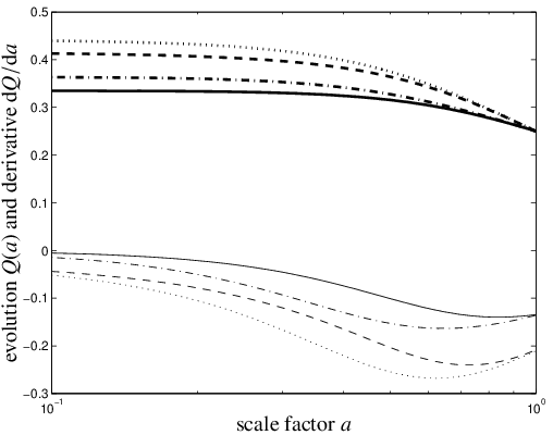
Physically, the expression for $Q(a)$ corresponds to the three ways in which models with CDM decay generate higher amplitudes for the iSW-effect, compared to models with stable CDM: Apart from the growth factor $D_{+}(a)$ and the Hubble function $H(a)$ (due to the time derivative of $D_{+}$), the matter density has had higher values in the past, and hence the fluctuations in the gravitational potentials generated by the overdensity field $\delta$ are stronger, which is described by $\Omega_{m}(a)$. Further interesting points include:

• •

  The derivative $\mathrm{d}Q/\mathrm{d}a$ in fact vanishes in the SCDM cosmology with $\Omega_{m}(a)=1$, $D_{+}(a)=a$ and $h(a)=a^{-3/2}$, because $Q(a)\equiv 1$ in this case. It is perhaps even more illustrative to look directly at the expression for $\mathrm{d}Q/\mathrm{d}a$ (eqn. 11) which is zero in SCDM cosmologies because (i) the logarithmic derivative of the Hubble function $H(a)$ is equal $-3/2$ (reflecting the matter domination), (ii) the logarithmic derivative of the matter density parameter vanishes (due to the stability of CDM), and the logarithmic derivative of the growth function $D_{+}(a)$ is equal to one (a combination of the two). From this point of view, both the growth proportional to $a$ and stable CDM are the necessary conditions that make the linear iSW-effect disappear in Einstein-de Sitter universes.

• •

  The two cosmologies $\Lambda$CDM and $\phi_{\Gamma}$CDM, which are almost degenerate in terms of their growth rates, give rise to very different $Q(a)$ and $\mathrm{d}Q/\mathrm{d}a$ functions, which is a result of the their dependence on $H(a)$ and $\Omega_{m}(a)$, and hence to a different iSW-effect.

• •

  In models with no coupling between the dark fluids, the matter density decreases $\rho_{m}(a)\propto a^{-3}$, and

  $$\frac{\Omega_{m}(a)}{\Omega_{m}}=\frac{H_{0}^{2}}{a^{3}H^{2}(a)}$$

  (12)

  applies. This allows the reformulation of the comoving Poisson equation in the familiar form,

  $$\Delta\Phi=\frac{3H_{0}^{2}\Omega_{m}}{2a}\delta.$$

  (13)

  Substitution into the line of sight integral yields the familiar equation for the iSW-effect in spatially flat dark energy cosmologies:

  $$\tau=\frac{3H_{0}^{2}\Omega_{m}}{c^{3}}\int_{0}^{\chi_{H}}\mathrm{d}\chi\>a^{2}H(a)\left(\frac{\mathrm{d}}{\mathrm{d}a}\frac{D_{+}}{a}\right)\Delta^{-1}\delta,$$

  (14)

  and $Q(a)$ reduces to $\Omega_{m}D_{+}(a)/a$ with a constant $\Omega_{m}$.

• •

  An analogous consideration applies to gravitational lensing: The weak lensing convergence $\kappa$ in coupled models reads

  $$\kappa=\frac{3}{2c^{2}}\int_{0}^{\chi_{H}}\mathrm{d}\chi\>a^{2}H^{2}(a)\Omega_{m}(a)\>G(\chi)\chi\>D_{+}\delta,$$

  (15)

  which replaces the common expression (Schneider et al., 1992; Bartelmann & Schneider, 2001),

  $$\kappa=\frac{3H_{0}^{2}\Omega_{m}}{2c^{2}}\int_{0}^{\chi_{H}}\mathrm{d}\chi\>G(\chi)\chi\>\frac{D_{+}}{a}\delta.$$

  (16)

  $G(\chi)$ is the lensing efficiency function of the background galaxy sample, which itself is influenced by the Hubble function $H(a)$.

The derivation above holds for general coupled cosmologies and is not restricted to the case of CDM decay, for which I exemplarily compute the iSW-spectra in the next chapter.

References

- Abramowitz & Stegun (1972) Abramowitz M., Stegun I. A., 1972, Handbook of Mathematical Functions. Handbook of Mathematical Functions, New York: Dover, 1972
- Bardeen et al. (1986) Bardeen J. M., Bond J. R., Kaiser N., Szalay A. S., 1986, ApJ, 304, 15
- Bartelmann & Schneider (2001) Bartelmann M., Schneider P., 2001, Physics Reports, 340, 291
- Boehmer et al. (2008) Boehmer C. G., Caldera-Cabral G., Lazkoz R., Maartens R., 2008, ArXiv 0801.1565, 801
- Boughn & Crittenden (2003) Boughn S. P., Crittenden R. G., 2003, in Holt S. H., Reynolds C. S., eds, The Emergence of Cosmic Structure Vol. 666 of American Institute of Physics Conference Series, The Absence of the Integrated Sachs-Wolfe Effect: Constraints on a Cosmological Constant. pp 67–70
- Chimento et al. (2003) Chimento L. P., Jakubi A. S., Pavón D., Zimdahl W., 2003, Phys. Rev. D, 67, 083513
- Cooray (2002) Cooray A., 2002, Phys. Rev. D, 65, 083518
- Crittenden & Turok (1996) Crittenden R. G., Turok N., 1996, Physical Review Letters, 76, 575
- Douspis et al. (2008) Douspis M., Castro P. G., Caprini C., Aghanim N., 2008, ArXiv 0802.0983, 802
- Fosalba et al. (2003) Fosalba P., Gaztañaga E., Castander F. J., 2003, ApJL, 597, L89
- Giannantonio et al. (2006) Giannantonio T., Crittenden R. G., Nichol R. C., Scranton R., Richards G. T., Myers A. D., Brunner R. J., Gray A. G., Connolly A. J., Schneider D. P., 2006, Phys. Rev. D, 74, 063520
- Giannantonio et al. (2008) Giannantonio T., Scranton R., Crittenden R. G., Nichol R. C., Boughn S. P., Myers A. D., Richards G. T., 2008, ArXiv 0801.4380, 801
- He & Wang (2008) He J.-H., Wang B., 2008, ArXiv 0801.4233, 801
- Hu & Sugiyama (1994) Hu W., Sugiyama N., 1994, Phys. Rev. D, 50, 627
- La Vacca & Colombo (2008) La Vacca G., Colombo L. P. L., 2008, ArXiv 0803.1640, 803
- Limber (1954) Limber D. N., 1954, ApJ, 119, 655
- Linder & Jenkins (2003) Linder E. V., Jenkins A., 2003, MNRAS, 346, 573
- Olivares et al. (2007) Olivares G., Atrio-Barandela F., Pavon D., 2007, ArXiv 0706.3860, 706
- Olivares et al. (2008) Olivares G., Atrio-Brandela F., Pavon D., 2008, ArXiv 0801.4517, 801
- Pettorino & Baccigalupi (2008) Pettorino V., Baccigalupi C., 2008, ArXiv 0802.1086, 802
- Rassat et al. (2007) Rassat A., Land K., Lahav O., Abdalla F. B., 2007, MNRAS, 377, 1085
- Rees & Sciama (1968) Rees M. J., Sciama D. W., 1968, Nature, 217, 511
- Refregier & the DUNE collaboration (2008) Refregier A., the DUNE collaboration 2008, ArXiv 0802.2522, 802
- Sachs & Wolfe (1967) Sachs R. K., Wolfe A. M., 1967, ApJ, 147, 73
- Schäfer & Bartelmann (2006) Schäfer B. M., Bartelmann M., 2006, MNRAS, 369, 425
- Schäfer et al. (2008) Schäfer B. M., Caldera Cabral G. A., Maartens R., 2008, ArXiv 0803.2232, 803
- Schneider et al. (1992) Schneider P., Ehlers J., Falco E. E., 1992, Gravitational Lenses. Springer-Verlag Berlin Heidelberg New York.
- Smith et al. (2003) Smith R. E., Peacock J. A., Jenkins A., White S. D. M., Frenk C. S., Pearce F. R., Thomas P. A., Efstathiou G., Couchman H. M. P., 2003, MNRAS, 341, 1311
- Turner & White (1997) Turner M. S., White M., 1997, Phys. Rev. D, 56, 4439
- Wang & Steinhardt (1998) Wang L., Steinhardt P. J., 1998, ApJ, 508, 483