\toappear

Conditioning Probabilistic Databases

Christoph Koch

Dan Olteanu Address: Department of Computer Science Address: Cornell University Address: Ithaca, NY 14853, USA Address: koch@cs.cornell.edu Address: Computing Laboratory Address: Oxford University Address: Oxford, OX1 3QD, UK Address: dan.olteanu@comlab.ox.ac.uk

Abstract

Past research on probabilistic databases has studied the problem of answering queries on a static database. Application scenarios of probabilistic databases however often involve the conditioning of a database using additional information in the form of new evidence. The conditioning problem is thus to transform a probabilistic database of priors into a posterior probabilistic database which is materialized for subsequent query processing or further refinement. It turns out that the conditioning problem is closely related to the problem of computing exact tuple confidence values.

It is known that exact confidence computation is an NP-hard problem. This has led researchers to consider approximation techniques for confidence computation. However, neither conditioning nor exact confidence computation can be solved using such techniques. In this paper we present efficient techniques for both problems. We study several problem decomposition methods and heuristics that are based on the most successful search techniques from constraint satisfaction, such as the Davis-Putnam algorithm. We complement this with a thorough experimental evaluation of the algorithms proposed. Our experiments show that our exact algorithms scale well to realistic database sizes and can in some scenarios compete with the most efficient previous approximation algorithms.

1 Introduction

Queries on probabilistic databases have numerous applications at the interface of databases and information retrieval [14], data cleaning [5], sensor data, tracking moving objects, crime fighting [6], and computational science [10].

A core operation of queries on probabilistic databases is the computation of confidence values of tuples in the result of a query. In short, the confidence in a tuple $t$ being in the result of a query on a probabilistic database is the combined probability weight of all possible worlds in which $t$ is in the result of the query.

By extending the power of query languages for probabilistic databases, new applications beyond the mere retrieval of tuples and their confidence become possible. An essential operation that allows for new applications is conditioning, the operation of removing possible worlds which do not satisfy a given condition from a probabilistic database. Subsequent query operations will apply to the reduced database, and a confidence computation will return conditional probabilities in the Bayesian sense with respect to the original database. Computing conditioned probabilistic databases has natural and important applications in virtually all areas in which probabilistic databases are useful. For example, in data cleaning, it is only natural to start with an uncertain database and then clean it – reduce uncertainty – by adding constraints or additional information. More generally, conditioning allows us to start with a database of prior probabilities, to add in some evidence, and take it to a posterior probabilistic database that takes the evidence into account.

Consider the example of a probabilistic database of social security numbers (SSN) and names of individuals extracted from paper forms using OCR software. If a symbol or word cannot be clearly identified, this software will offer a number of weighted alternatives. The database

R	SSN	NAME
	{ 1 (p=.2) $\mid$ 7 (p=.8) }	John
	{ 4 (p=.3) $\mid$ 7 (p=.7) }	Bill

represents four possible worlds (shown in Figure 1), modelling that John has either SSN 1 or 7, with probability .2 and .8 (the paper form may contain a hand-written symbol that can either be read as a European “1” or an American “7”), respectively, and Bill has either SSN 4 or 7, with probability .3 and .7, respectively. We assume independence between John’s and Bill’s alternatives, thus the world in which John has SSN 1 and Bill has SSN 7 has probability $.2\cdot.7=.14$ .

If $A_{x}$ denotes the event that Bill has SSN $x$ , then $P(A_{4})=.3$ and $P(A_{7})=.7$ . We can compute these probabilities in a probabilistic database by asking for the confidence values of the tuples in the result of the query

select SSN, conf(SSN) from R where NAME = ’Bill’;

which will result in the table

Q	SSN	CONF
	4	.3
	7	.7

$R^{1}$	SSN	NAME
	1	John
	4	Bill

$R^{2}$	SSN	NAME
	7	John
	4	Bill

P = .06

P = .24

$R^{3}$	SSN	NAME
	1	John
	7	Bill

$R^{4}$	SSN	NAME
	7	John
	7	Bill

P = .14

P = .56

Figure 1: The four worlds of the input database.

Now suppose we want to use the additional knowledge that social security numbers are unique. We can express this using a functional dependency SSN $\rightarrow$ NAME. Asserting this constraint, or conditioning the probabilistic database using the constraint, means to eliminate all those worlds in which the functional dependency does not hold.

Let $B$ be the event that the functional dependency holds. Conceptually, the database conditioned with $B$ is obtained by removing world $R^{4}$ (in which John and Bill have the same SSN) and renormalizing the probabilities of the remaining worlds to have them again sum up to 1, in this case by dividing by $.06+.24+.14=.44$ . We will think of conditioning as an operation assert[ $B$ ] that reduces uncertainty by declaring worlds in which $B$ does not hold impossible.

Computing tuple confidences for the above query on the original database will give us, for each possible SSN value $x$ for Bill, the probabilities $P(A_{x})$ , while on the database conditioned with $B$ it will give a table of social security numbers $x$ and conditional probabilities $P(A_{x}\mid B)$ . For example, the conditional probability of Bill having SSN 4 given that social security numbers are unique is

P(A_{4}\mid B)=\frac{P(A_{4}\land B)}{P(B)}=\frac{.3}{.44}\approx.68.

Using this definition, we could alternatively have computed the conditional probabilities by combining the results of two confidence computations,

select SSN, P1/P2
from	(	select SSN, conf(SSN) P1 from R, B
		where NAME = ’Bill’),
	(select conf() P2 from B);

where $B$ is a Boolean query that is true if the functional dependency holds on $R$ .

Unfortunately, both conditioning and confidence computation are NP-hard problems. Nevertheless, their study is justified by their obvious relevance and applications. While conditioning has not been previously studied in the context of probabilistic databases, previous work on confidence computation has aimed at cases that admit polynomial-time query evaluation and at approximating confidence values [10].

Previous work often assumes that confidence values are computed at the end of a query, closing the possible worlds semantics of the probabilistic database and returning a complete, nonprobabilistic relation of tuples with numerical confidence values that can be used for decision making. In such a context, techniques that return a reasonable approximation of confidence values may be acceptable.

In other scenarios we do not want to accept approximate confidence values because errors made while computing these estimates aggregate and grow, causing users to make wrong decisions based on the query results. This is particularly true in compositional query languages for probabilistic databases, where confidence values computed in a subquery form part of an intermediate result that can be accessed and used for filtering the data in subsequent query operations [20].

Similar issues arise when confidence values can be inserted into the probabilistic database through updates and may be used in subsequent queries. For example, data cleaning is a scenario where we, on one hand, want to materialize the result of a data transformation in the database once and for all (rather than having to redo the cleaning steps every time a query is asked) and on the other hand do not want to store incorrect probabilities that may affect a very large number of subsequent queries. Here we need techniques for conditioning and exactly computing confidence values.

Exact confidence computation is particularly important in queries in which confidence values are used in comparison predicates. For an example, let us add a third person, Fred, to the database whose SSN is either 1 or 4, with equal probability. If we again condition using the functional dependency SSN $\rightarrow NAME$ , we have only two possible worlds, one in which John, Bill, and Fred have social security numbers 1, 7, and 4, respectively, and one in which their SSN are 7, 4, and 1. If we now ask for the social security numbers that are in the database for certain,

select SSN from R where conf(SSN) = 1;

we should get three tuples in the result. Monte Carlo simulation based approximation algorithms will do very badly on such queries. Confidence approximation using a Karp-Luby-style algorithm [18, 10, 22] will independently underestimate each tuple’s confidence with probability $\approx$ .5. Thus the probability that at least one tuple is missing from the result of such a query is very high (see also [20].

In this paper, we develop efficient algorithms for computing exact confidences and for conditioning probabilistic databases. The detailed contributions are as follows.

•

In most previous models of probabilistic databases over finite world-sets, computing tuple confidence values essentially means the weighted counting of solutions to constraint structures closely related to disjunctive normal form formulas. Our notion of such structures are the world-set descriptor sets, or ws-sets for short. We formally introduce a probabilistic database model that is known to cleanly and directly generalize many previously considered probabilistic database models (cf. [4]) including, among others, various forms of tuple-independence models [10, 3], ULDBs [6], product decomposition [5], and c-table-based models [4]. We use this framework to study exact confidence computation and conditioning. The results obtained are thus of immediate relevance to all these models.
•

We study properties of ws-sets that are essential to relational algebra query evaluation and to the design of algorithms for the two main problems of the paper.
•

We exhibit the fundamental, close relationship between the two problems.
•

We develop ws-trees, which capture notions of structural decomposition of ws-sets based on probabilistic independence and world-set disjointness. Once a ws-tree has been obtained for a given ws-set, both exact confidence computation and conditioning are feasible in linear time. The main problem is thus to efficiently find small ws-tree decompositions.
•

To this end, we develop a decomposition procedure motivated by the Davis-Putnam (DP) procedure for checking Propositional Satisfiability [13]. DP, while many decades old, is still the basis of the best exact solution techniques for the NP-complete Satisfiability problem. We introduce two decomposition rules, variable elimination (the main rule of DP) and a new independence decomposition rule, and develop heuristics for chosing among the rules.
•

We develop a database conditioning algorithm based on ws-tree decompositions and prove its correctness.
•

We study ws-set simplification and elimination techniques that can be either used as an alternative to the DP-based procedure or combined with it.
•

We provide a thorough experimental evaluation of the algorithms presented in this paper. We also experimentally compare our exact techniques for confidence computation with approximation based on Monte Carlo simulation.

The structure of the paper follows the list of contributions.

2 Probabilistic Databases

Var	Dom	P
$j$	1	.2
$j$	7	.8
$b$	4	.3
$b$	7	.7

WSD	SSN	NAME
$\{j\mapsto 1\}$	1	John
$\{j\mapsto 7\}$	7	John
$\{b\mapsto 4\}$	4	Bill
$\{b\mapsto 7\}$	7	Bill

Figure 2: Probabilistic database with ws-descriptors made explicit and defined by world-table

W

We define sets of possible worlds following U-relational databases [4]. Consider a finite set of independent random variables ranging over finite domains. Probability distributions over the possible worlds are defined by assigning a probability $P(\{x\mapsto i\})$ to each assignment of a variable $x$ to a constant of its domain, $i\in\mbox{Dom}_{x}$ , such that the probabilities of all assignments of a given variable sum up to one. We represent the set of variables, their domains, and probability distributions relationally by a world-table $W$ consisting of all triples $(x,i,p)$ of variables $x$ , values $i$ in the domain of $x$ , and the associated probabilities $p=P(\{x\mapsto i\})$ .

A world-set descriptor is a set of assignments $x\mapsto i$ with $i\in\mbox{Dom}_{x}$ that is functional, i.e. a partial function from variables to domain values. If such a world-set descriptor $d$ is a total function, then it identifies a possible world. Otherwise, it denotes all those possible worlds $\omega(d)$ identified by total functions $f$ that can be obtained by extension of $d$ . (That is, for all $x$ on which $d$ is defined, $d(x)=f(x)$ .) Because of the independence of the variables, the aggregate probability of these worlds is

P(d)=\prod_{\{x\mapsto i\}\subseteq d}P(\{x\mapsto i\}).

If $d=\emptyset$ , then $d$ denotes the set of all possible worlds.

We say that two ws-descriptors $d_{1}$ and $d_{2}$ are consistent iff their union (as sets of assignments) is functional.

A ws-set is a set of ws-descriptors $S$ and represents the world-set computed as the union of the world-sets represented by the ws-descriptors in the set. We define the semantics of ws-sets using the (herewith overloaded) function $\omega$ extended to ws-sets, $\omega(S):=\underset{d\in S}{\bigcup}(\omega(d))$ .

A U-relation over schema $\Sigma$ and world-table $W$ is a set of tuples over $\Sigma$ , where we associate to each tuple a ws-descriptor over $W$ . A probabilistic database over schema $\{\Sigma_{1},\ldots,\Sigma_{n}\}$ and world-table $W$ is a set of $n$ U-relations, each over one schema $\Sigma_{i}$ and $W$ . A probabilistic database represents a set of databases, one database for each possible world defined by $W$ . To obtain a possible world in the represented set, we first choose a total valuation $f$ over $W$ . We then process each probabilistic relation $R_{i}$ tuple by tuple. If $f$ extends the ws-descriptor $d$ of a tuple $t$ , then $t$ is in the relation $R_{i}$ of that database.

Example 2.1

Consider again the probabilistic database of social security numbers and names given in Figure 1. Its representation in our formalism is given in Figure 2. The world-table $W$ of Figure 2 defines two variables $j$ and $b$ modeling the social security numbers of John and Bill, with domains $\{1,7\}$ and $\{4,7\}$ respectively. The probability of the world defined by $f=\{j\mapsto 7,b\mapsto 7\}$ is $.8\cdot.7=.56$ . The total valuation $f$ extends the ws-descriptors of the second and fourth tuple of relation $U_{R}$ , thus the relation $R$ in world $f$ is { (7, John), (7, Bill) }. $\hskip 0.0pt\Box$

Remark 2.2

Leaving aside the probability distributions of the variables which are represented by the $W$ table, U-relations are essentially restricted c-tables [17] in which the global condition is “true”, variables must not occur in the tuples, and each local condition must be a conjunction of conditions of the form $x=v$ where x is a variable and $v$ is a constant. Nevertheless, it is known that U-relations are a complete representation system for probabilistic databases over nonempty finite sets of possible worlds.

U-relations can be used to represent attribute-level uncertainty using vertically decomposed relations. For details on this, we refer to [4]. All results in this paper work in the context of attribute-level uncertainty.

The efficient execution of the operations of positive relational algebra on such databases was described in that paper as well. Briefly, if U-relations $U_{R}$ and $U_{S}$ represent relations $R$ and $S$ , then selections $\sigma_{\phi}R$ and projections $\pi_{\overline{A}}R$ simply translate into $\sigma_{\phi}U_{R}$ and $\pi_{WSD,\overline{A}}U_{R}$ , respectively. Joins $R\bowtie_{\phi}S$ translate into $U_{R}\bowtie_{\phi\land\psi}U_{S}$ where $\psi$ is the condition that the ws-descriptors of the two tuples compared are consistent with each other (i.e., have a common extension into a total valuation). The set operations easily follow from the analogous operations on ws-sets that will be described below, in Section 3.2. $\hskip 0.0pt\Box$

Example 2.3

The functional dependency SSN $\rightarrow$ NAME on the probabilistic database of Figure 2 can be expressed as a boolean relational algebra query as the complement of $\pi_{\emptyset}(R\bowtie_{\phi}R)$ where $\phi:=(1.SSN=2.SSN\land 1.NAME\neq 2.NAME)$ . We turn this into the query

\pi_{WSD}(U_{R}\bowtie_{\phi\land 1.WSD\;\mathrm{consistent\ with}\;2.WSD}U_{R}).

over our representation, which results in the ws-set $\{j\mapsto 7,b\mapsto 7\}$ . The complement of this with the world-set given by the $W$ relation, $\{\{j\mapsto 1\},\{j\mapsto 7\},\{b\mapsto 4\},\{b\mapsto 7\}\}$ , is $\{\{j\mapsto 1\},\{j\mapsto 7,b\mapsto 4\}\}$ . (Note that this is just one among a set of equivalent solutions.) $\hskip 0.0pt\Box$

3 Properties of ws-descriptors

In this section we investigate properties of ws-descriptors and show how they can be used to efficiently implement various set operations on world-sets without having to enumerate the worlds. This is important, for such sets can be extremely large in practice: [5, 4] report on experiments with $10^{10^{6}}$ worlds.

3.1 Mutex, Independence, and Containment

Two ws-descriptors $d_{1}$ and $d_{2}$ are (1) mutually exclusive (mutex for short) if they represent disjunct world-sets, i.e., $\omega(d_{1})\cap\omega(d_{2})=\emptyset$ , and (2) independent if there is no valuation of the variables in one of the ws-descriptors that restricts the set of possible valuations of the variables in the other ws-descriptor (that is, $d_{1}$ and $d_{2}$ are defined only on disjoint sets of variables). A ws-descriptor $d_{1}$ is contained in $d_{2}$ if the world-set of $d_{1}$ is contained in the world-set of $d_{2}$ , i.e., $\omega(d_{1})\subseteq\omega(d_{2})$ . Equivalence is mutual containment.

Although ws-descriptors represent very succinctly possibly very large world-sets, all aforementioned properties can be efficiently checked at the syntactical level: $d_{1}$ and $d_{2}$ , where all variables with singleton domains are eliminated, are (1) mutex if there is a variable with a different assignment in each of them, and (2) independent if they have no variables in common; $d_{1}$ is contained in $d_{2}$ if $d_{1}$ extends $d_{2}$ .

Example 3.1

Consider the world-table of Figure 2 and the ws-descriptors $d_{1}=\{j\mapsto 1\}$ , $d_{2}=\{j\mapsto 7\}$ , $d_{3}=\{j\mapsto 1,b\mapsto 4\}$ , and $d_{4}=\{b\mapsto 4\}$ . Then, the pairs $(d_{1},d_{2})$ and $(d_{2},d_{3})$ are mutex, $d_{3}$ is contained in $d_{1}$ , and the pairs $(d_{1},d_{4})$ and $(d_{2},d_{4})$ are independent. $\hskip 0.0pt\Box$

We also consider the mutex, independence, and equivalence properties for ws-sets. Two ws-sets $S_{1}$ and $S_{2}$ are mutex (independent) iff $d_{1}$ and $d_{2}$ are mutex (independent) for any $d_{1}\in S_{1}$ and $d_{2}\in S_{2}$ . Two ws-sets are equivalent if they represent the same world-set.

Example 3.2

We continue Example 3.1. The ws-set $\{d_{1}\}$ is mutex with $\{d_{2}\}$ . $\{d_{1},d_{2}\}$ is independent from $\{d_{4}\}$ . At a first glance, it looks like $\{d_{1},d_{2}\}$ and $\{d_{3},d_{4}\}$ are neither mutex nor independent, because $d_{1}$ and $d_{3}$ overlap. However, we note that $d_{3}\subseteq d_{4}$ and then $\omega(\{d_{3},d_{4}\})=\omega(\{d_{4}\})$ and $\{d_{4}\}$ is independent from $\{d_{1},d_{2}\}$ . $\hskip 0.0pt\Box$

3.2 Set Operations on ws-sets

Various relevant computation tasks, ranging from decision procedures like tuple possibility [2] to confidence computation of answer tuples, and conditioning of probabilistic databases, require symbolic manipulations of ws-sets. For example, checking whether two tuples of a probabilistic relation can co-occur in some worlds can be done by intersecting their ws-descriptors; both tuples co-occur in the worlds defined by the intersection of the corresponding world-sets.

We next define set operations on ws-sets.

•

Intersection. $\mbox{Intersect}(S_{1},S_{2}):=$

$\{d_{1}\cap d_{2}\mid d_{1}\in S_{1},d_{2}\in S_{2},d_{1}\mbox{ is consistent with }d_{2}\}.$
•

Union. $\mbox{Union}(S_{1},S_{2}):=S_{1}\cup S_{2}$ .

•

Difference. The definition is inductive, starting with singleton ws-sets. If ws-descriptors $d_{1}$ and $d_{2}$ are inconsistent, $\mbox{Diff}(\{d_{1}\},\{d_{2}\}):=\{d_{1}\}.$ Otherwise,

\mbox{Diff}(\{d_{1}\},\{d_{2}\}):=\\ \{d_{1}\cup\{x_{1}\mapsto w_{1},\dots,x_{i-1}\mapsto w_{i-1},x_{i}\mapsto w^{\prime}_{i}\}\mid\\ d_{2}-d_{1}=\{x_{1}\mapsto w_{1},\dots,x_{k}\mapsto w_{k}\},\\ 1\leq i\leq k,w^{\prime}_{i}\in\mbox{dom}_{x_{i}},w_{i}\neq w^{\prime}_{i}\}.

\mbox{Diff}(\{d_{1}\},S\cup\{d_{2}\}):=\mbox{Diff}(\mbox{Diff}(\{d_{1}\},S),\{d_{2}\}).

\mbox{Diff}(\{d_{1},\dots,d_{n}\},S):=\bigcup_{1\leq i\leq n}\mbox{Diff}(\{d_{i}\},S).

Example 3.3

Consider $d_{1}=\{j\mapsto 1\}$ , $d_{2}=\{j\mapsto 7\}$ , and $d_{3}=\{j\mapsto 1,b\mapsto 4\}$ . Then, $\mbox{Intersect}(\{d_{1}\},\{d_{2}\})=\mbox{Intersect}(\{d_{2}\},\{d_{3}\})=\emptyset$ because $d_{2}$ is inconsistent with $d_{1}$ and $d_{3}$ . $\mbox{Intersect}(\{d_{1}\},\{d_{3}\})=\{d_{3}\}$ , because $d_{3}$ is contained in $d_{1}$ . $\mbox{Diff}(\{d_{2}\},\{d_{1}\})=\mbox{Diff}(\{d_{2}\},\{d_{3}\})=\{d_{2}\}$ because $d_{2}$ is mutex with $d_{1}$ and $d_{3}$ . $\mbox{Diff}(\{d_{1}\},\{d_{3}\})=\{\{j\mapsto 1,b\mapsto 7\}\}$ . $\mbox{Diff}(\{d_{3}\},\{d_{1}\})=\{d_{3}\}$ , because $d_{3}$ and $d_{1}$ are inconsistent. $\hskip 0.0pt\Box$

Proposition 3.4

The above definitions of set operations on ws-sets are correct:

1.

$\omega(\mbox{Union}(S_{1},S_{2}))=\omega(S_{1})\cup\omega(S_{2})$ .
2.

$\omega(\mbox{Intersect}(S_{1},S_{2}))=\omega(S_{1})\cap\omega(S_{2})$ .
3.

$\omega(\mbox{Diff}(S_{1},S_{2}))=\omega(S_{1})-\omega(S_{2})$ .

The ws-descriptors in $\mbox{Diff}(S_{1},S_{2})$ are pairwise mutex.

V	D	P
$x$	1	.1
$x$	2	.4
$x$	3	.5
$y$	1	.2
$y$	2	.8
$z$	1	.4
$z$	2	.6
$u$	1	.7
$u$	2	.3
$v$	1	.5
$v$	2	.5

pstree{TR{\otimes}}{pstree{TR{\oplus}}{TR{\emptyset}^{x\mapsto 1}pstree{TR{\otimes}_{x\mapsto 2}}{pstree{TR{\oplus}}{TR{\emptyset}^{y\mapsto 1}}pstree{TR{\oplus}}{TR{\emptyset}_{z\mapsto 1}}}}pstree{TR{\oplus}}{pstree{TR{\oplus}^{u\mapsto 1}}{TR{\emptyset}_{v\mapsto 1}}TR{\emptyset}_{u\mapsto 2}}}

$S=\{$
	$\{x\mapsto 1\}$ ,
	$\{x\mapsto 2,y\mapsto 1\}$ ,
	$\{x\mapsto 2,z\mapsto 1\}$ ,
	$\{u\mapsto 1,v\mapsto 1\}$ ,
	$\{u\mapsto 2\}$
$\}$

Figure 3: World-set table

W

, a ws-tree

R

over

W

, and an equivalent ws-set

S

4 World-set trees

The ws-sets have important properties, like succinctness, closure under set operations, and natural relational encoding, and [4] employed them to achieve the purely relational processing of positive relational algebra on U-relational databases. When it comes to the manipulation of probabilities of query answers or of worlds violating given constraints, however, ws-sets are in most cases inadequate. This is because ws-descriptors in a ws-set may represent non-disjoint world-sets, and for most manipulations of probabilities a substantial computational effort is needed to identify common world-subsets across possibly many ws-descriptors.

We next introduce a new compact representation of world-sets, called world-set tree representation, or ws-tree for short, that makes the structure in the ws-sets explicit. This representation formalism allows for efficient exact probability computation and conditioning and has strong connections to knowledge compilation, as it is used in system modelling and verification [12]. There, too, various kinds of decision diagrams, like binary decision diagrams (BDDs) [8], are employed for the efficient manipulation of propositional formulas.

Definition 4.1

Given a world-table $W$ , a ws-tree over $W$ is a tree with inner nodes $\otimes$ and $\oplus$ , leaves holding the ws-descriptor $\emptyset$ , and edges annotated with weighted variable assignments consistent with $W$ . The following constraints hold for a ws-tree:

•

A variable defined in $W$ occurs at most once on each root-to-leaf path.
•

Each of its $\oplus$ -nodes is associated with a variable $v$ such that each outgoing edge is annotated with a different assignment of $v$ .
•

The sets of variables occurring in the subtrees rooted at the children of any $\otimes$ -node are disjoint. $\hskip 0.0pt\Box$

We define the semantics of ws-trees in strict analogy to that of ws-sets based on the observation that the set of edge annotations on each root-to-leaf path in a ws-tree represents a ws-descriptor. The world-set represented by a ws-tree is precisely represented by the ws-set consisting of the annotation sets of all root-to-leaf paths. The inner nodes have a special semantics: the children of a $\otimes$ -node use disjoint variable sets and are thus independent, and the children of a $\oplus$ -node follow branches with different assignments of the same variable and are thus mutually exclusive.

Example 4.2

Figure 3 shows a ws-tree and the ws-set consisting of all its root-to-leaf paths. $\hskip 0.0pt\Box$

$\displaystyle\hskip-20.00003pt\underline{\mbox{ComputeTree}}\mbox{ (WS-Set S) returns WS-Tree}$ $\displaystyle\mbox{\bf\ if }(S=\emptyset)\mbox{\bf\ then return }\bot$ $\displaystyle\mbox{\bf\ else if }(\emptyset\in S)\hskip 10.00002pt\mbox{//S contains a universal ws-desc}$ $\displaystyle\hskip 20.00003pt\mbox{\bf\ then return }\emptyset$ else choose one of the following: (independent partitioning) if there are non-empty and independent ws-sets $\displaystyle\hskip 10.00002ptS_{1},\dots,S_{|I|}\mbox{\bf\ such that }S=S_{1}\cup\dots\cup S_{|I|}$ $\displaystyle\mbox{\bf\ then return }\underset{i\in I}{\bigotimes}\big(\mbox{ComputeTree}(S_{i})\big)$ (variable elimination) $\displaystyle\mbox{choose a variable }x\mbox{ in }S;$ $\displaystyle T:=\{d\mid d\in S,\not\exists i\in\mathrm{dom}_{x}:\{x\mapsto i\}\subseteq d\};$ $\displaystyle\forall i\in\mathrm{dom}_{x}:S_{x\mapsto i}:=\{\{y_{1}\mapsto j_{1},\ldots,y_{m}\mapsto j_{m}\}\mid$ $\displaystyle\hskip 50.00008pt\{x\mapsto i,y_{1}\mapsto j_{1},\ldots,y_{m}\mapsto j_{m}\}\in S\};$ $\displaystyle\mbox{\bf\ return }\underset{i\in\mathrm{dom}_{x}}{\bigoplus}\big(x\mapsto i:\mbox{ComputeTree}(S_{x\mapsto i}\cup T)\big)$

Figure 4: Translating ws-sets into ws-trees.

4.1 Constructing world-set trees

The key idea underlying our translation of ws-sets into ws-trees is a divide-and-conquer approach that exploits the relationships between ws-descriptors, like independence and variable sharing.

Figure 4 gives our translation algorithm. We proceed recursively by partitioning the ws-sets into independent disjoint partitions (when possible) or into (possibly overlapping) partitions that are consistent with different assignments of a variable. In the case of independent partitioning, we create $\otimes$ -nodes whose children are the translations of the independent partitions. In the second case, we simplify the problem by eliminating a variable: we choose a variable $x$ and create an $\oplus$ -node whose outgoing edges are annotated with different assignments $x\mapsto i$ of $x$ and whose children are translations of the subsets of the ws-set consisting of ws-descriptors consistent with $x\mapsto i$ ¹¹ 1 Our translation abstracts out implementation details. For instance, for those assignments of $x$ that do not occur in $S$ we have $T\cup S_{x\mapsto i}=T$ and can translate $T$ only once.. If at any recursion step the input ws-set contains the nullary ws-descriptor, which by definition represents the whole world-set, then we stop from recursion and create a ws-tree leaf $\emptyset$ . This can happen after several variable elimination steps that reduced some of the input ws-descriptors to $\emptyset$ .

Example 4.3

We show how to translate the ws-set $S$ into the ws-tree $R$ (Figure 3). We first partition $S$ into two (minimally) independent ws-sets $S_{1}$ and $S_{2}$ : $S_{1}$ consists of the first three ws-descriptors of $S$ , and $S_{2}$ consists of the remaining two. For $S_{1}$ , we can eliminate any of the variables $x$ , $y$ , or $z$ . Consider we choose $x$ and create two branches for $x\mapsto 1$ and $x\mapsto 2$ respectively (there is no ws-descriptor consistent with $x\mapsto 3$ ). For the first branch, we stop with the ws-set $\{\emptyset\}$ , whereas for the second branch we continue with the ws-set $\{\{y\mapsto 1\},\{z\mapsto 1\}\}$ . The latter ws-set can be partitioned into independent subsets in the context of the assignment $x\mapsto 2$ . We proceed similarly for $S_{2}$ and choose to eliminate variable $u$ . We create an $\oplus$ -node with outgoing edges for assignments $u\mapsto 1$ and $u\mapsto 2$ respectively. We are left in the former case with the ws-set $\{\{v\mapsto 1\}\}$ and in the latter case with $\{\emptyset\}$ .

Different variable choices can lead to different ws-trees. This is the so-called variable ordering problem that applies to the construction of binary decision diagrams. Later in this section we discuss heuristics for variable orderings. $\hskip 0.0pt\Box$

Theorem 4.4

Given a ws-set $S$ , ComputeTree( $S$ ) and $S$ represent the same world-set.

Our translation can yield ws-trees of exponential size (similar to BDDs). This rather high worst-case complexity needs to be paid for efficient exact probability computation and conditioning. It is known that counting models of propositional formulas and exact probability computation are #P-hard problems [10]. This complexity result does not preclude, however, BDDs from being very successful in practice. We expect the same for ws-trees. The key observation for a good behaviour in practice is that we should partition ws-sets into independent subsets whenever possible and we should carefully choose a good ordering for variable eliminations. Both methods greatly influence the size of the ws-trees and the translation time, as shown in the next example.

pstree{TR{\oplus}}{pstree{TR{\oplus}^{y\mapsto 1}}{pstree{TR{\otimes}^{u\mapsto 1}}{pstree{TR{\oplus}}{TR{\emptyset}^{v\mapsto 1}}pstree{TR{\oplus}}{pstree{TR{\oplus(\alpha)}^{z\mapsto 2}}{TR{\emptyset}^{x\mapsto 1}TR{\emptyset}_{x\mapsto 2}}TR{\alpha}}}TR{\emptyset}_{u\mapsto 2}}pstree{TR{\oplus}_{y\mapsto 2}}{TR{\emptyset}^{x\mapsto 1}pstree{TR{\otimes}_{\hskip-16.48907ptx\mapsto 2}}{pstree{TR{\oplus}}{TR{\emptyset}^{z\mapsto 1\mbox{ }}}pstree{TR{\oplus(\beta)}}{TR{\emptyset}^{u\mapsto 2}pstree{TR{\oplus}_{u\mapsto 1}}{TR{\emptyset}_{v\mapsto 1}}}}TR{\beta}_{\mbox{ }x\mapsto 3}}}

Figure 5: A ws-tree equivalent to

R

of Figure 3.

Example 4.5

Consider again the ws-set $S$ of Figure 3 and a different ordering for variable eliminations that leads to the ws-tree of Figure 5. We shortly discuss the construction of this ws-tree. Assume we choose to eliminate the variable $y$ and obtain the ws-sets

	$\displaystyle S_{y\mapsto 2}$	$\displaystyle=\{\{x\mapsto 1\},\{x\mapsto 2,z\mapsto 1\},\{u\mapsto 1,v\mapsto 1\},\{u\mapsto 2\}\}$
	$\displaystyle S_{y\mapsto 1}$	$\displaystyle=S_{y\mapsto 2}\cup\{\{x\mapsto 2\}\}$

In contrast to the computation of the ws-tree $R$ of Figure 3, our variable choice creates intermediary ws-sets that overlap at large, which ultimately leads to a large increase in the size of the ws-tree. This bad choice need not necessarily lead to redundant computation, which we could easily detect. In fact, the only major savings in case we detect and eliminate redundancy here are the subtrees $\alpha$ and $\beta$ , which still leave a graph larger than $R$ . $\hskip 0.0pt\Box$

Estimate (WS-Set $S$ , variable $x$ in $S$ ) returns Real missing_assignment := false; foreach $i\in\mathrm{dom}_{x}$ do compute $S_{x\mapsto i}$ and $T$ as shown in Figure 4 if $|S_{x\mapsto i}|>0$ then $s_{i}=|S_{x\mapsto i}\cup T|$ else $s_{i}=0$ ; missing_assignment = true; endif if (missing_assignment) then $e=|T|$ else $e=0$ foreach $j\in\mathrm{dom}_{x}$ such that $s_{j}>0$ do $e=e+\log_{k}(1+k^{s_{j}-e})$ return $e$

Figure 6: Log cost estimate for a variable choice.

4.2 Heuristics

We next study heuristics for variable elimination and independent partitioning that are compared experimentally in Section 7. We devise a simple cost estimate, which we use to decide at each step whether to partition or which variable to eliminate. We assume that, in worst case, the cost of translating a ws-set $S$ is $2^{|S|}$ (following the exponential formula of the inclusion-exclusion principle).

In case of independent partitioning, the partitions $S_{1},\ldots,$ $S_{n}$ are disjoint and can be computed in polynomial time (by computing the connected components of the graph of variables co-occurring within ws-descriptors). We thus reduce the computation cost from $2^{|S|}$ to $2^{|S_{1}|}+\cdots+2^{|S_{n}|}$ . This method is, however, not always applicable and we need to apply variable elimination.

The main advantage of variable elimination is that $S$ is divided into subsets $T\cup S_{x\mapsto i}$ without the dependencies enforced by variable $x$ and thus subject to independent partitioning in the context of $x\mapsto i$ . Consider $s_{i}$ the size of the ws-set $T\cup S_{x\mapsto i}$ . Then, the cost of choosing $x$ is $\underset{i\in\mathrm{dom}_{x}}{\Sigma}2^{s_{i}}$ . Of course, for those assignments of $x$ that do not occur in $S$ we have $T\cup S_{x\mapsto i}=T$ and can translate $T$ only once. The computation cost using variable elimination can match that of independent partitioning only in the case that the assignments of the chosen variable partition the input ws-set $S$ and thus $T$ is empty.

Our first heuristic, called minlog, chooses a variable that minimizes $\log(\underset{i=1}{\overset{\mathrm{dom}_{x}}{\Sigma}}2^{s_{i}})$ . Figure 6 shows how to compute incrementally the cost estimate by avoiding summation of potentially large numbers. The variable missing_assignment is used to detect whether there is at least one assignment of $x$ not occuring in $S$ for which $T$ will be translated; in this case, $T$ is only translated once (and not for every missing assignment).

The second heuristic, called minmax, approximates the cost estimate and chooses a variable that minimizes the maximal ws-set $T\cup S_{x\mapsto i}$ . Both heuristics need time linear in the sizes of all variable domains plus of the ws-set. In addition to minmax, minlog needs to perform log and exp operations.

Remark 4.6

To better understand our heuristics, we give one scenario where minmax behaves suboptimal. Consider $S$ of size $n$ and two variables. Variable $x$ occurs with the same assignment in $n-1$ ws-descriptors and thus its minmax estimate is $n$ , and variable $y$ occurs twice with different assignments, and thus its minmax estimate is $n-1$ . Using minmax, we choose $y$ , although the minlog would choose differently: $e(y)=\log(2\cdot 2^{n-1}+2^{n-2})>\log(2\cdot 2^{n-1})=e(x)$ . $\hskip 0.0pt\Box$

$\displaystyle P\big(\bigotimes_{i\in I}S_{i}\big)$ $\displaystyle=1-\prod_{i\in I}(1-P(S_{i}))$ $\displaystyle P\big(\bigoplus_{i\in I}(x\mapsto i:S_{i})\big)$ $\displaystyle=\sum_{i\in I}P(\{x\mapsto i\})\cdot P(S_{i})$ $\displaystyle P(\emptyset)$ $\displaystyle=1\hskip 40.00006ptP(\bot)=0$

Figure 7: Probability computation for ws-trees.

4.3 Probability computation

We next give an algorithm for computing the exact probability of a ws-set by employing the translation of ws-sets into ws-trees discussed in Section 4. Figure 7 defines the function $P$ to this effect. This function is defined using pattern matching on the node types of ws-trees. The probability of an $\otimes$ -node is the joint probability of its independent children $S_{1},\ldots,S_{|I|}$ . The probability of an $\oplus$ -node is the joint probability of its mutually exclusive children, where the probability of each child $S_{i}$ is weighted by the probability of the variable assignment $x\mapsto i$ annotating the incoming edge of $S_{i}$ . Finally, the probability of a leaf represented by the nullary ws-descriptor is 1 and of $\bot$ is 0.

Example 4.7

The probability of the ws-tree $R$ of Figure 3 can be computed as follows (we label the inner nodes with $l$ for left child and $r$ for right child):

	$\displaystyle P(R)$	$\displaystyle=1-(1-P(l))\cdot(1-P(r))$
	$\displaystyle P(l)$	$\displaystyle=P(\{x\mapsto 1\})\cdot P(\emptyset)+P(\{x\mapsto 2\})\cdot P(lr)$
	$\displaystyle P(lr)$	$\displaystyle=1-(1-P(\{y\mapsto 1\})\cdot P(\emptyset))\cdot(1-P(\{z\mapsto 1\})\cdot P(\emptyset))$
	$\displaystyle P(r)$	$\displaystyle=P(\{u\mapsto 1\})\cdot P(\{v\mapsto 1\})\cdot P(\emptyset)+P(\{u\mapsto 2\})\cdot P(\emptyset)$

We can now replace the probabilities for variable assignments and ws-descriptor $\emptyset$ and obtain

	$\displaystyle P(r)$	$\displaystyle=0.7\cdot 0.5\cdot 1+0.3=0.65$
	$\displaystyle P(lr)$	$\displaystyle=1-(1-0.2\cdot 1)\cdot(1-0.4\cdot 1)=0.52$
	$\displaystyle P(l)$	$\displaystyle=0.1\cdot 1+0.4\cdot 0.52=0.308$
	$\displaystyle P(R)$	$\displaystyle=1-(1-0.308)\cdot(1-0.65)=0.7578\hskip 60.00009pt\Box$

The probability of a ws-tree $R$ can be computed in one bottom-up traversal of $R$ and does not require the precomputation of $R$ . The translation and probability computation functions can be easily composed to obtain the function $\mbox{ComputeTree}\circ P$ by inlining $P$ in ComputeTree. As a result, the construction of the nodes $\oplus$ , $\otimes$ , and $\emptyset$ is replaced by the corresponding probability computation given by $P$ .

5 Conditioning

In this section we study the problem of conditioning a probabilistic database, i.e., the problem of removing all possible worlds that do not satisfy a given condition (say, by a Boolean relational calculus query) and renormalizing the database such that, if there is at least one world left, the probability weights of all worlds sum up to one.

We will think of conditioning as a query or update operation assert_ϕ, where $\phi$ is the condition, i.e., a Boolean query. Processing relational algebra queries on probabilistic databases was discussed in Section 2. We will now assume the result of the Boolean query given as a ws-set defining the worlds on which $\phi$ is true.

Example 5.1

Consider again the data cleaning example from the Introduction, formalized by the U-relational database of Figure 2. Relation $W$ represents the set of possible worlds and $U$ represents the tuples in these worlds.

As discussed in Example 2.3, the set of ws-descriptors $S=\{\{j\mapsto 1\},\{j\mapsto 7,b\mapsto 4\}\}$ represents the three worlds on which the functional dependency SSN $\rightarrow$ NAME holds. The world $\{j\mapsto 7,b\mapsto 7\}$ is excluded and thus the confidence of $S$ does not add up to one but to $.2+.8\cdot.3=.44$ . What we now want to do is transform this database into one that represents the three worlds identified by $S$ and preserves their tuples as well as their relative weights, but with a sum of world weights of one. This can of course be easily achieved by multiplying the weight of each of the three remaining worlds by 1/.44. However, we want to do this in a smart way that in general does not require to consider each possible world individually, but instead preserves a succinct representation of the data and runs efficiently.

Such a technique exists and is presented in this section. It is based on running our confidence computation algorithm for ws-trees and, while returning from the recursion, renormalizing the world-set by introducing new variables whose assignments are normalized using the confidence values obtained. For this example, the conditioned database will be

Var	Dom	P
$b$	4	.3
$b$	7	.7
$j^{\prime}$	1	.2/.44
$j^{\prime}$	7	$.8\cdot.3/.44$

WSD	SSN	NAME
$\{j^{\prime}\mapsto 1\}$	1	John
$\{j^{\prime}\mapsto 7\}$	7	John
$\{j^{\prime}\mapsto 1,b\mapsto 4\}$	4	Bill
$\{j^{\prime}\mapsto 1,b\mapsto 7\}$	7	Bill
$\{j^{\prime}\mapsto 7\}$	4	Bill

Note that the $W$ relation actually models four possible worlds, but two of them, $\{j^{\prime}\mapsto 7,b\mapsto 4\}$ and $\{j^{\prime}\mapsto 7,b\mapsto 7\}$ are equal (contain the same tuples). Example 5.2 will show in detail how conditioning works. $\hskip 0.0pt\Box$

cond: conditioning algorithm In: ws-tree $R$ representing the new nonempty world-set, ws-set $U$ from the U-relations Out: (confidence value, ws-set $U^{\prime}$ ) if $R=\emptyset$ then return $(1,U)$ ; if $R=\underset{i\in I}{\bigotimes}\big(R_{i}\big)$ then foreach $i\in I$ do $(c_{i},U_{i}):=\mbox{cond}(R_{i},U)$ ; return $(1-\prod_{i}(1-c_{i}),\underset{i\in I}{\bigcup}U_{i})$ ; if $R=\underset{i\in\mbox{dom}_{x}}{\bigoplus}\big(x\mapsto i:R_{i}\big)$ then foreach $i\in\mbox{dom}_{x}$ do $U_{i}:=$ the subset of $U$ consistent with $x\mapsto i$ ; $(c_{i},U^{\prime}_{i}):=\mbox{cond}(R_{i},U_{i})$ ; $c:=\sum_{i\in I}P(\{x\mapsto i\})\cdot c_{i}$ ; let $x^{\prime}$ be a new variable; foreach $i\in\mbox{dom}_{x}$ such that $c_{i}\not=0$ do add ${\langle x^{\prime},i,\frac{P(\{x\mapsto i\})\cdot c_{i}}{c}\rangle}$ to the $W$ relation; replace each occurrence of $x$ in $U_{i}^{\prime}$ by $x^{\prime}$ ; return $(c,\underset{i\in\mbox{dom}_{x}}{\bigcup}U_{i}^{\prime})$ ;

Figure 8: The conditioning algorithm.

$U$	WSD	A
	$\{y\mapsto 2,u\mapsto 1\}$	$a_{1}$
	$\{u\mapsto 1,v\mapsto 2\}$	$a_{2}$

$\Delta W$	Var	Dom	P
	$x^{\prime}$	1	.1/.308
	$x^{\prime}$	2	.208/.308
	$y^{\prime}$	1	1
	$z^{\prime}$	1	1
	$u^{\prime}$	1	.35/.65
	$u^{\prime}$	2	.3/.65
	$v^{\prime}$	1	1

pstree{TR{\otimes}}{pstree{TR{\oplus}}{TR{\emptyset}^{x^{\prime}\stackrel{{\scriptstyle\frac{.1}{.308}}}{{\mapsto}}1}pstree{TR{\otimes}_{x^{\prime}\stackrel{{\scriptstyle\frac{.208}{.308}}}{{\mapsto}}2}}{pstree{TR{\oplus}}{TR{\emptyset}^{y^{\prime}\stackrel{{\scriptstyle 1}}{{\mapsto}}1}}pstree{TR{\oplus}}{TR{\emptyset}_{z^{\prime}\stackrel{{\scriptstyle 1}}{{\mapsto}}1}}}}pstree{TR{\oplus}}{pstree{TR{\oplus}^{u^{\prime}\stackrel{{\scriptstyle\frac{.35}{.65}}}{{\mapsto}}1}}{TR{\emptyset}_{v^{\prime}\stackrel{{\scriptstyle 1}}{{\mapsto}}1}}TR{\emptyset}_{u^{\prime}\stackrel{{\scriptstyle\frac{.3}{.65}}}{{\mapsto}}2}}}

Figure 9: U-relation

U

, additions

\Delta W

to the

W

-relation, and a renormalized ws-tree.

Figure 8 gives our efficient algorithm for conditioning a U-relational database. The input is a U-relational database and a ws-tree $R$ that describes the subset of the possible worlds of the database that we want to condition it to. The output is a modified U-relational database and, as a by-product, since we recursively need to compute confidences for the renormalization, the confidence of $R$ in the input database. The confidence of $R$ in the output database will of course be 1. The renormalization works as follows. The probability of each branch of an inner node $n$ of $R$ is re-weighted such that the probability of $n$ becomes 1. We reflect this re-weighting by introducing new variable whose assignments reflect the new weights of the branches of $n$ .

This algorithm is essentially the confidence computation algorithm of Figure 7. We just add some lines of code along the line of recursively computing confidence that renormalize the weights of alternative assignments of variables for which some assignments become impossible. Additionally, we pass around a set of ws-descriptors (associated with tuples from the input U-relational database) and extend each ws-descriptor in that set by $x\mapsto i$ whenever we eliminate variable $x$ , for each of its alternatives $i$ .

Example 5.2

Consider the U-relational database consisting of the $W$ -relation of Figure 3 and the U-relation $U$ of Figure 9. Let us run the algorithm to condition the database on the ws-tree $R$ of Figure 3 ( $R$ need not be precomputed for conditioning).

We recursively call function cond at each node in the ws-tree $R$ starting at the root. To simplify the explanation, let us assume a numbering of the nodes and of the ws-sets we pass around: If $R_{w}$ is a (sub)tree then $R_{w,i}$ is its $i$ -th child. The ws-set passed in the recursion with $R_{w}$ is $U_{w}$ and the ws-set returned is $U^{\prime}_{w}$ . The ws-sets passed on at the nodes of $R$ are:

	$\displaystyle U_{1}$	$\displaystyle=U_{2}=U$
	$\displaystyle U_{1,1}$	$\displaystyle=x\mapsto 1:U=\{\{x\mapsto 1,y\mapsto 2,u\mapsto 1\},$
		$\displaystyle\hskip 20.00003pt\{x\mapsto 1,u\mapsto 1,v\mapsto 2\}\}$
	$\displaystyle U_{1,2}$	$\displaystyle=x\mapsto 2:U=\{\{x\mapsto 2,y\mapsto 2,u\mapsto 1\},$
		$\displaystyle\hskip 20.00003pt\{x\mapsto 2,u\mapsto 1,v\mapsto 2\}\}$
	$\displaystyle U_{1,2,1,1}$	$\displaystyle=y\mapsto 1:U_{1,2}=\{\{y\mapsto 1,x\mapsto 2,u\mapsto 1,v\mapsto 2\}\}$
	$\displaystyle U_{1,2,2,1}$	$\displaystyle=z\mapsto 1:U_{1,2}=\{\{z\mapsto 1,x\mapsto 2,y\mapsto 2,u\mapsto 1\},$
		$\displaystyle\hskip 20.00003pt\{z\mapsto 1,x\mapsto 2,u\mapsto 1,v\mapsto 2\}\}$
	$\displaystyle U_{2,1}$	$\displaystyle=u\mapsto 1:U_{2}=U_{2}$
	$\displaystyle U_{2,2}$	$\displaystyle=u\mapsto 2:U_{2}=\emptyset$
	$\displaystyle U_{2,1,1}$	$\displaystyle=v\mapsto 1:U_{2,1}=\{\{v\mapsto 1,y\mapsto 2,u\mapsto 1\}\}$

When we reach the leaves of $R$ , we start returning from recursion and do the following. We first compute the probabilities of the nodes of $R$ – in this case, they are already computed in Example 4.7. Next, for each $\oplus$ -node representing the elimination of a variable, say $\alpha$ , we create a new variable $\alpha^{\prime}$ with the assignments of $\alpha$ present at that node. In contrast to $\alpha$ , the assignments of $\alpha^{\prime}$ are re-weighted by the probability of that $\oplus$ -node so that the sum of their weights is 1. The new variables and their weighted assignments are given in Figure 9 along the original ws-tree $R$ and in the $\Delta W$ relation to be added to the world table $W$ .

When we return from recursion, we also compute the new ws-sets $U^{\prime}_{i}$ from $U_{i}$ . These ws-sets are equal in case of leaves and $\otimes$ -nodes, but, in case of $\oplus$ -nodes, the variable eliminated at that node is replaced by the new one we created. In case of $\oplus$ and $\otimes$ nodes, we also return the union of all $U^{\prime}_{i}$ of their children. We finally return from the first call with the following ws-set $U^{\prime}$ :

	$\displaystyle\{$	$\displaystyle\{x^{\prime}\mapsto 1,y\mapsto 2,u\mapsto 1\},$
		$\displaystyle\{x^{\prime}\mapsto 1,u\mapsto 1,v\mapsto 2\},$
		$\displaystyle\{x^{\prime}\mapsto 2,y^{\prime}\mapsto 1,u\mapsto 1,v\mapsto 2\},$
		$\displaystyle\{x^{\prime}\mapsto 2,z^{\prime}\mapsto 1,y\mapsto 2,u\mapsto 1\},$
		$\displaystyle\{x^{\prime}\mapsto 2,z^{\prime}\mapsto 1,u\mapsto 1,v\mapsto 2\},$
		$\displaystyle\{u^{\prime}\mapsto 1,v^{\prime}\mapsto 1,y\mapsto 2\}\}.$

$\hskip 0.0pt\Box$

Let us view a probabilistic database semantically, as a set of pairs $(I,p)$ of instances $I$ with probability weights $p$ .

Theorem 5.3

Given a representation of probabilistic database ${\bf W}=\{(I_{1},p_{1}),\dots,(I_{n},p_{n})\}$ and a ws-tree $R$ identifying a nonempty subset of the worlds of W, the algorithm of Figure 8 computes a representation of probabilistic database

\{(I_{j},\frac{p_{j}}{c})\mid(I_{j},p_{j})\in{\bf W},I_{j}\in\omega(R)\}

such that the probabilities $p_{j}$ add up to 1.

Thus, of course, $c$ is the confidence of $R$ .

Three simple optimizations of this algorithm that simplify the world table $W$ and the output ws-descriptors are worth mentioning.

1.

Variables that do not appear anywhere in the U-relations can be dropped from $W$ .
2.

Variables with a single domain value (obviously of weight 1) can be dropped everywhere from the database.
3.

Variables $x^{\prime}$ and $x^{\prime\prime}$ obtained from the same variable $x$ (by creation of a new variable in the case of variable elimination on $x$ in two distinct branches of the recursion) can be merged into the same variable if the alternatives and their weights in the $W$ relation are the same. In that case we can replace $x^{\prime\prime}$ by $x^{\prime}$ everywhere in the database.

Example 5.4

In the previous example, we can remove the variables $y^{\prime},z^{\prime}$ , and $v^{\prime}$ from the $W$ -relation and all variable assignments involving these variables from the U-relation because of (1). Furthermore, we can remove the variables $x$ and $z$ because of (1). The resulting database is

$U^{\prime}$	WSD	A
	$\{x^{\prime}\mapsto 1,y\mapsto 2,u\mapsto 1\}$	$a_{1}$
	$\{x^{\prime}\mapsto 1,u\mapsto 1,v\mapsto 2\}$	$a_{2}$
	$\{x^{\prime}\mapsto 2,u\mapsto 1,v\mapsto 2\}$	$a_{2}$
	$\{x^{\prime}\mapsto 2,y\mapsto 2,u\mapsto 1\}$	$a_{1}$
	$\{x^{\prime}\mapsto 2,u\mapsto 1,v\mapsto 2\}$	$a_{2}$
	$\{u^{\prime}\mapsto 1,y\mapsto 2\}$	$a_{1}$

Var	Dom	P
$x^{\prime}$	1	.1/.308
$x^{\prime}$	2	.208/.308
$y$	1	.2
$y$	2	.8
$u$	1	.7
$u$	2	.3
$u^{\prime}$	1	.35/.65
$u^{\prime}$	2	.3/.65
$v$	1	.5
$v$	2	.5

Finally, we state an important property of conditioning (expressed by the assert operation) useful for query optimization.

Theorem 5.5

Assert-operations commute with other asserts and the operations of positive relational algebra.

6 ws-descriptor elimination

We next present an alternative to exact probability computation using ws-trees based on the difference operation on ws-sets, called here ws-descriptor elimination. The idea is to incrementally eliminate ws-descriptors from the input ws-set. Given a ws-set $S$ and a ws-descriptor $d_{1}$ in $S$ , we compute two ws-sets: the original ws-set $S$ without $d_{1}$ , and the ws-set representing the difference of $\{d_{1}\}$ and the first ws-set. The probability of $S$ is then the sum of the probabilities of the two computed ws-sets, because the two ws-sets are mutex, as stated below by function $P_{w}$ :

	$\displaystyle P_{w}(\emptyset)$	$\displaystyle=0\hskip 40.00006ptP_{w}(\{\emptyset\})=1$
	$\displaystyle P_{w}(S)$	$\displaystyle=P_{w}(\{d_{2},\ldots,d_{n}\})+\underset{d\in(\{d_{1}\}-\{d_{2},\ldots,d_{n}\})}{\sum}P(d)$

The function $P$ computes here the probability of a ws-descriptor.

Example 6.1

Consider the ws-set $\{d_{1},d_{2},d_{3}\}$ of Example 3.1. The ws-descriptor $d_{2}$ is mutex with both $d_{1}$ and $d_{3}$ and we can eliminate it: $P_{w}(\{d_{1},d_{2},d_{3}\})=P_{w}(\{d_{1},d_{3}\})+P(d_{2})$ . We now choose any to eliminate $d_{3}$ and obtain $P_{w}(\{d_{1},d_{3}\})=P_{w}(\{d_{3}\}-\{d_{1}\})+P(d_{1})=P(d_{1})$ , as explained in Example 3.3. Thus $P_{w}(\{d_{1},d_{2},d_{3}\})=P(d_{2})+P(d_{1})=1$ . $\hskip 0.0pt\Box$

This method exploits the fact that the difference operation preserves the mutex property and is world-set monotone.

Lemma 6.2

The following equations hold for any ws-sets $S_{1}$ , $S_{2}$ , and $S_{3}$ :

$\displaystyle\omega(S_{1}-S_{2})$	$\displaystyle\subseteq$	$\displaystyle\omega(S_{1})$
$\displaystyle\omega(S_{1})\cup\omega(S_{2})$	$\displaystyle=$	$\displaystyle\omega(S_{1}-S_{2})\cup\omega(S_{2})$
$\displaystyle\emptyset$	$\displaystyle=$	$\displaystyle\omega(S_{1}-S_{2})\cap\omega(S_{2})$
$\displaystyle\omega(S_{1})\cap\omega(S_{2})=\emptyset$	$\displaystyle\Rightarrow$	$\displaystyle\omega(S_{1}-S_{3})\cap\omega(S_{2}-S_{3})=\emptyset$

The correctness of probability computation by ws-descriptor elimination follows immediately from Lemma 6.2.

Theorem 6.3

Given a ws-set $S$ , the function $P_{w}$ computes the probability of $S$ .

As a corollary, we have that

Corollary 6.4 (Theorem 6.3)

Any ws-set $\overset{n}{\underset{i=1}{\bigcup}}\{d_{i}\}$ has the equivalent mutex ws-set $\overset{n-1}{\underset{i=1}{\bigcup}}(\{d_{i}\}-\overset{n}{\underset{j=i+1}{\bigcup}}\{d_{j}\})\cup\{d_{n}\}$ .

Like the translation of ws-sets into ws-trees, this method can take exponential time in the size of the input ws-set. Moreover, the equivalent mutex ws-set given above can be exponential. On the positive side, computing the exact probability of such mutex ws-sets can be done in linear time. Additionally, the probability of $\{d\}-S_{d}$ can be computed on the fly without requiring to first generate all ws-descriptors in the difference ws-set. This follows from the fact that the difference operation on ws-descriptors only generates mutex and distinct ws-descriptors. After generating a ws-descriptor from the difference ws-set we can thus add its probability to a running sum and discard it before generating the next ws-descriptor. The next section reports on experiments with an implementation of this method.

7 Experiments

Query	Size of	TPC-H	#Input	Size of	User
	ws-desc.	Scale	Vars	ws-set	Time(s)
$Q_{1}$ : select true from customer c, orders o, lineitem l		0.01	77215	9836	5.10
where c.mktsegment $=$ ’BUILDING’ and c.custkey $=$ o.custkey	3	0.05	382314	43498	99.76
and o.orderkey $=$ l.orderkey and o.orderdate $>$ ’1995-03-15’		0.10	765572	63886	356.56
$Q_{2}$ : select true from lineitem		0.01	60175	3029	0.20
where shipdate between ’1994-01-01’ and ’1996-01-01’	1	0.05	299814	15545	8.24
and discount between ’0.05’ and ’0.08’ and quantity $<$ 24		0.10	600572	30948	33.68

Figure 10: TPC-H scenario: Queries, data characteristics, and performance of INDVE(minlog).

Refer to caption — Figure 11: The two cases when the numbers of variables and of ws-descriptors differ by orders of magnitude.

The experiments were conducted on an Athlon-X2 (4600+) x86-64bit/1.8GB/ Linux 2.6.20/gcc 4.1.2 machine.

We considered two synthetic data sets.

TPC-H data and queries. The first data set consists of tuple-independent probabilistic databases obtained from relational databases produced by TPC-H 2.7.0, where each tuple is associated with a Boolean random variable and the probability distribution is chosen at random. We evaluated the two Boolean queries of Figure 10 on each probabilistic database and then computed the probability of the ws-set consisting of the ws-descriptors of all the answer tuples. Among the two queries, only the second is safe and thus admits PTIME evaluation on tuple-independent probabilistic databases [10]. As we rewrite constraints into Boolean queries, we consider this querying scenario equally relevant to conditioning.

#P-hard cases. The second data set consists of ws-sets similar to those associated with the answers of nonhierarchical conjunctive queries without self-joins on tuple-independent probabilistic databases, i.e. join queries such as $Q_{s}=R_{1}\Join\dots\Join R_{s}$ for schemas $R_{i}(A_{i},A_{i+1})$ in which all relations are joined together, but there is no single column common to all of them. Such queries are known to be #P-hard [10].

The data generation is simple: we partition the set of variables into $s$ equally-sized sets $V_{1},\dots,V_{s}$ and then sample ws-sets $\{x_{1}\mapsto a_{1},\dots,x_{s}\mapsto a_{s}\}$ where $x_{i}$ is from $V_{i}$ and $a_{i}$ is a random alternative for $x_{i}$ , for $1\leq i\leq s$ . It is easy to verify that each such ws-set is actually the result of query $Q_{s}$ on some tuple-independent probabilistic database. (For $s=3$ this fact is used in the #P-hardness proof of [10].)

We use the following parameters in our experiments: number $n$ of variables ranging from 50 to 100K, number $r$ of possible alternatives per variable (2 or 4), length $s$ of ws-descriptors, which equals the number of joined relations (2 or 4), and number $w$ of ws-descriptors ranging from 5 to 60K. For each variable, the alternatives have uniform probabilities $1/r$ : our exact algorithms are not sensitive to changing probability values as long as the numbers of alternatives of the variables remain constant.

Note that the focus on Boolean queries means no loss of generality for confidence computation; rather, the projection of a query result to a nullary relation causes all the ws-sets to be unioned and large.

Algorithms. We experimentally compared three versions of our exact algorithm: one that employs independent partitioning and variable elimination (INDVE), one that employs variable elimination only (VE), and one with ws-descriptor elimination (WE). We considered INDVE with the two heuristics minlog and minmax. These implementations compute confidence values and the modified world table ( $\Delta W$ in Example 5.2), but do not materialize the modified, conditioned U-relations ( $U^{\prime}$ in Example 5.2). We have verified that the computation of these additional data structures adds only a small overhead over confidence computation in practice. We therefore do not distinguish in the sequel between confidence computation and conditioning. Note that our implementation is based on the straightforward composition of the ComputeTree and conditioning algorithms and does not need to materialize the ws-trees.

Although we also implemented a brute-force algorithm for probability computation, its timing is extremely bad and not reported. At a glance, this algorithm iterates over all worlds and sums up the probabilities of those that are represented by some ws-descriptors in the input ws-set. We also tried a slight improvement of the brute-force algorithm by first partitioning the input ws-set into independent subsets [23]. This version, too, performed bad and is not reported, as the partitioning can only be applied once at the beginning on the whole ws-set, yet most of our input ws-sets only exhibit independence in the context of variable eliminations.

We experimentally compared INDVE against a Monte Carlo simulation algorithm for confidence computation [22, 10] which is based on the Karp-Luby (KL) fully polynomial randomized approximation scheme (FPRAS) for DNF counting [18]. Given a DNF formula with $m$ clauses, the base algorithm computes an $(\epsilon,\delta)$ -approximation $\hat{c}$ of the number of solutions $c$ of the DNF formula such that

\Pr[|c-\hat{c}|\leq\epsilon\cdot c]\geq 1-\delta

for any given $0<\epsilon<1$ , $0<\delta<1$ . It does so within $\lceil 4\cdot m\cdot\log(2/\delta)/\epsilon^{2}\rceil$ iterations of an efficiently computable estimator. This algorithm can be easily turned into an $(\epsilon,\delta)$ -FPRAS for tuple confidence computation (see [20]). In our experiments, we use the optimal Monte-Carlo estimation algorithm of [9]. This is a technique to determine a small sufficient number of Monte-Carlo iterations (within a constant factor from optimal) based on first collecting statistics on the input by running the Monte Carlo simulation a small number of times. We use the version of the Karp-Luby unbiased estimator described in the book [25], which converges faster than the basic algorithm of [18], adapted to the problem of computing confidence values. This algorithm is similar to the self-adjusting coverage algorithm of [19].

1. Queries on TPC-H data. Figure 10 shows that INDVE(minlog) performs within hundreds of seconds in case of queries with equi-joins ( $Q_{1}$ ) and selection-projection ( $Q_{2}$ ) on tuple-independent probabilistic TPC-H databases with over 700K variables and 60K ws-descriptors. In the answers of query $Q_{2}$ , ws-descriptors are pairwise independent, and INDVE can effectively employ independence partitition, making confidence computation more efficient than for $Q_{1}$ .

The remaining experiments use the second data generator.

2. The numbers of variables and of ws-descriptors differ by orders of magnitude. If there are much more ws-descriptors than variables, many ws-descriptors share variables (or variable assignments) and a good choice for variable elimination can effectively partition the ws-set. On the other hand, independence partitioning is unlikely to be very effective, and the time for checking it is wasted. Figure 11(a) shows that in such cases VE and INDVE (with minlog heuristic) are very stable and not influenced by fluctuations in data correlations. In particular, VE performs better than INDVE and within a second for 100 variables with domain size 4 (and nearly the same for 2), ws-descriptors of length 4, and ws-set size above 1.2k. We witnessed a sharp hard-easy transition at 1.2k, which suggests that the computation becomes harder when the number of ws-descriptors falls under one order of magnitude greater than the number of variables. Experiment 3 studies easy-hard-easy transitions in more detail. The plot data were produced from 25 runs and record the median value and ymin/ymax for the error bars.

In case of many variables and few ws-descriptors, the independence partitioning clearly pays off. This case naturally occurs for query evaluation on probabilistic databases, where a small set of tuples (and thus of ws-descriptors) is selected from a large database. As shown in Figure 11(b), INDVE(minlog) performs within seconds for the case of 100K variables and 100 to 6K ws-descriptors of size $s=2$ , and with variable domain size $r=4$ . Two further findings are not shown in the figure: (1) VE performs much worse than INDVE, as it cannot exploit the independence of tuples and thus creates partitions that overlap at large; (2) the case of $s=4$ has a few (2 in 25) outliers exceeding 600 seconds.

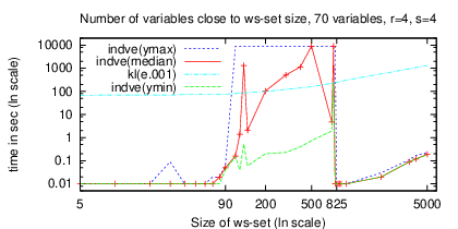
3. The numbers of variables and of ws-descriptors are close. It is known from literature on knowledge compilation and model counting [7] that the computation becomes harder in this case. Figure 12 shows the easy-hard-easy pattern of INDVE(minlog) by plotting the minimal, maximal, and median computation time of 20 runs (max allowed time of 9000s). We experimentally observed the expected sharp transitions: When the numbers of ws-descriptors and of variables become close, the computation becomes hard and remains so until the number of ws-descriptors becomes one order of magnitude larger than the number of variables. The behavior of WE (not shown in the figure) follows very closely the easy-hard transition of INDVE, but in our experiment WE does not return anymore to the easy case within the range of ws-set sizes reported on in the figure.

4. Exact versus approximate computation. We experimentally verified our conjecture that the Karp-Luby approximation algorithm (KL) converges rather slowly. In case the numbers of variables and of ws-descriptors differ by orders of magnitude, INDVE(minlog) and VE(minlog) are definitely competitive when compared to KL with parameters $\epsilon=0.1$ resp. $\epsilon=0.01$ , and $\delta=0.01$ , see Figure 11.

In Figure 11(b), KL uses about the same number of iterations for all the ws-set sizes, a sufficient number to warrant the running time. The reason for the near-constant line for KL is that for $s=2$ and 100k variables, ws-descriptors are predominantly pairwise independent, and the confidence is close to $1-(3/4)^{w}$ , where $w$ is the number of ws-descriptors. But this quickly gets close to 1, and the optimal algorithm can decide on a small number of iterations that does not increase with $w$ . In case the numbers of variables and ws-descriptors are close (Figure 12), KL with $\epsilon=0.001$ only performs better than INDVE(minlog) in the hard cases.

5. Heuristics for variable elimination. Figure 13 shows that, although the minmax heuristic is cheaper to compute than the minlog heuristic, using minlog we find in general better choices of variables and INDVE remains less sensitive to data correlations. The plot data are produced from 10 runs and show the median value and ymin/ymax for the error bars. Although VE exceeds the allocated time of 600 seconds for different data points, it does this less than five times (the median value is closer to ymin).

8 Related Work

To the best of our knowledge, this paper is the first to study the conditioning problem for probabilistic databases. In this section, we survey related work in the areas of probabilistic databases and knowledge compilation procedures.

U-relations capture most other representation formalisms for uncertain data that were recently proposed in the literature, including those of MystiQ [10], Trio [6], and MayBMS [4]. For each of these formalisms, natural applications in data cleaning and other areas have been described [6, 5, 10].

Graphical models are a class of rich formalisms for representing probabilistic information which perform well in scenarios in which conditional probabilities and a known graph of dependencies and independences between events are available. There are, for instance, Bayesian network learning algorithms that produce just such data. Unfortunately, if probabilistic data is obtained by queries on tuple-independent or similar databases, the corresponding graphical models tend to be relatively flat [24] but have high tree-width, which causes techniques widely used for confidence computation on graphical models to be highly inefficient. Graphical models are more succinct than U-relations, yet their succinctness does not benefit the currently known query evaluation techniques. This justifies the development of conditioning techniques specifically for the c-table-like representations (such as U-relations) developed by the database community.

It has been long known that computing tuple confidence values on DNF-like representations of sets of possible worlds is a generalization of the DNF model counting problem and is #P-complete [11]. Monte Carlo approximation techniques for confidence computation have been known since the original work by Karp, Luby, and Madras [19]. Within the database field, this approach has first been followed in work on query reliability [15] and in the MystiQ project [10]. Section 7 reports on an experimental comparison of approximation and our exact algorithms.

Our variable elimination technique is based on Davis-Putnam procedure for satisfiability checking [13]. This procedure was already used for model counting [7]. Our approach combines it with independent partitioning for efficiently solving two more difficult problems: exact confidence computation and conditioning. [7] uses the minmax heuristic (which we benchmark against) and discusses experiments for CNF formulas with up to 50 variables and 200 clauses only. Our experiments also discuss new settings that are more natural in a database context: for instance, when the size of a query answer (and thus the number of ws-descriptors) is small in comparison to the size of the input database (and thus of variables). Follow-up work [16] reports on techniques for compiling ws-sets generated by conjunctive queries with inequalities into decision diagrams with polynomial-time guarantees.

Finally, there is a strong connection between ws-trees and ordered binary decision diagrams (OBDDs). Both make the structure of the propositional formulas explicit and allow for efficient manipulation. They differ, however, in important aspects: binary versus multistate variables, same variable ordering on all paths in case of OBDDs, and the new ws-tree $\otimes$ -node type, which makes independence explicit. It is possible to reduce the gap between the two formalisms, but this affects the representation size. For instance, different variable orderings on different paths allows for exponentially more succinct BDDs [21]. Multistate variables can be easily translated into binary variables at a price of a logarithmic increase in the number of variables [26].

References

[2] S. Abiteboul, P. Kanellakis, and G. Grahne. “On the Representation and Querying of Sets of Possible Worlds”. Theor. Comput. Sci., 78(1):158–187, 1991.
[3] P. Andritsos, A. Fuxman, and R. J. Miller. “Clean Answers over Dirty Databases: A Probabilistic Approach”. In Proc. ICDE, 2006.
[4] L. Antova, T. Jansen, C. Koch, and D. Olteanu. “Fast and Simple Relational Processing of Uncertain Data”. In Proc. ICDE, 2008.
[5] L. Antova, C. Koch, and D. Olteanu. “ $10^{10^{6}}$ Worlds and Beyond: Efficient Representation and Processing of Incomplete Information”. In Proc. ICDE, 2007.
[6] O. Benjelloun, A. D. Sarma, A. Halevy, and J. Widom. “ULDBs: Databases with Uncertainty and Lineage”. In Proc. VLDB, 2006.
[7] E. Birnbaum and E. Lozinskii. “The Good Old Davis-Putnam Procedure Helps Counting Models”. Journal of AI Research, 10(6):457–477, 1999.
[8] R. E. Bryant. Graph-based algorithms for boolean function manipulation. IEEE Trans. Computers, 35(8):677–691, 1986.
[9] P. Dagum, R. M. Karp, M. Luby, and S. M. Ross. “An Optimal Algorithm for Monte Carlo Estimation”. SIAM J. Comput., 29(5):1484–1496, 2000.
[10] N. Dalvi and D. Suciu. “Efficient query evaluation on probabilistic databases”. VLDB Journal, 16(4):523–544, 2007.
[11] N. Dalvi and D. Suciu. “Management of Probabilistic Data: Foundations and Challenges”. In Proc. PODS, 2007.
[12] A. Darwiche and P. Marquis. “A knowlege compilation map”. Journal of AI Research, 17:229–264, 2002.
[13] M. Davis and H. Putnam. “A Computing Procedure for Quantification Theory”. Journal of ACM, 7(3):201–215, 1960.
[14] N. Fuhr and T. Rölleke. “A Probabilistic Relational Algebra for the Integration of Information Retrieval and Database Systems”. ACM Trans. Inf. Syst., 15(1):32–66, 1997.
[15] E. Grädel, Y. Gurevich, and C. Hirsch. “The Complexity of Query Reliability”. In Proc. PODS, pages 227–234, 1998.
[16] J. Huang and D. Olteanu. Conjunctive queries with inequalities on probabilistic databases. Technical report, University of Oxford, 2008.
[17] T. Imielinski and W. Lipski. “Incomplete information in relational databases”. Journal of ACM, 31(4):761–791, 1984.
[18] R. M. Karp and M. Luby. “Monte-Carlo Algorithms for Enumeration and Reliability Problems”. In Proc. FOCS, pages 56–64, 1983.
[19] R. M. Karp, M. Luby, and N. Madras. “Monte-Carlo Approximation Algorithms for Enumeration Problems”. J. Algorithms, 10(3):429–448, 1989.
[20] C. Koch. “Approximating Predicates and Expressive Queries on Probabilistic Databases”. In Proc. PODS, 2008.
[21] C. Meinel and T. Theobald. Algorithms and Data Structures in VLSI Design. Springer-Verlag, 1998.
[22] C. Re, N. Dalvi, and D. Suciu. Efficient top-k query evaluation on probabilistic data. In Proc. ICDE, pages 886–895, 2007.
[23] A. D. Sarma, M. Theobald, and J. Widom. “Exploiting Lineage for Confidence Computation in Uncertain and Probabilistic Databases”. In Proc. ICDE, 2008.
[24] P. Sen and A. Deshpande. “Representing and Querying Correlated Tuples in Probabilistic Databases”. In Proc. ICDE, pages 596–605, 2007.
[25] V. V. Vazirani. Approximation Algorithms. Springer, 2001.
[26] M. Wachter and R. Haenni. “Multi-state Directed Acyclic Graphs”. In Proc. Canadian AI, pages 464–475, 2007.

Proof of Theorem 4.4

We prove that the translation from ws-sets to ws-trees is correct. That is, given a ws-set $S$ , ComputeTree( $S$ ) and $S$ represent the same world-set.

We use induction on the structure of ws-trees. In the base case, we map ws-sets representing the empty world-set to $\bot$ , and ws-sets containing the universal ws-descriptor $\emptyset$ (that represents the whole world-set) to $\emptyset$ . We consider now a ws-set $S$ . We have two cases corresponding to the different types of ws-tree inner nodes.

Case 1. Assume $S=\underset{i\in I}{\bigcup}S_{i}$ with $S_{i}$ pairwise independent and $R_{i}=\mbox{ComputeTree}(S_{i})$ . By hypothesis, $\omega(R_{i})=\omega(S_{i})$ . Then, $\mbox{ComputeTree}(S)=\underset{i\in I}{\bigotimes}(R_{i})$ and $\omega(\mbox{ComputeTree}(S))=\underset{i\in I}{\bigcup}\omega(R_{i})=\underset{i\in I}{\bigcup}\omega(S_{i})=\omega(S).$

Case 2. Let $x$ be a variable in $S$ and consider the ws-sets $S_{x\mapsto i}$ ( $i\in\mbox{dom}_{x}$ ) and $T$ as given by ComputeTree. Because the whole world-set can be represented by $A=\underset{i\in\mbox{dom}_{x}}{\bigcup}\{\{x\mapsto i\}\}$ , it holds that $\omega(A)\cap\omega(S)=\omega(S)$ . We push the assignments of $x$ in each ws-descriptor of $S$ and obtain

\omega(S)=\omega\big(\underset{i\in\mbox{dom}_{x}}{\bigcup}\{d\cup\{x\mapsto i\}\mid d\in S\}\big).

We can remove all inconsistent ws-descriptors in the ws-set of the right-hand side while preserving equivalence:

		$\displaystyle\omega(\{d\cup\{x\mapsto i\}\mid d\in S\})=$
		$\displaystyle\omega(\{d\cup\{x\mapsto i\}\mid d\in S,\not\exists j\in\mbox{dom}_{x}:j\not=i,\{x\mapsto j\}\subseteq d\})=$
		$\displaystyle\omega(\{d\cup\{x\mapsto i\}\mid\{x\mapsto i\}\subseteq d\in S\})\cup$
		$\displaystyle\omega(\{d\cup\{x\mapsto i\}\mid d\in S,\not\exists j\in\mbox{dom}_{x}:\{x\mapsto j\}\subseteq d\})=$
		$\displaystyle\omega(S_{x\mapsto i})\cup\omega(T)=\omega(S_{x\mapsto i}\cup T)$

We now consider all values $i\in\mbox{dom}_{x}$ and obtain

	$\displaystyle\omega(S)$	$\displaystyle=\omega\big(\underset{i\in\mbox{ dom}_{x}}{\bigcup}(S_{x\mapsto i}\cup T)\big)$
		$\displaystyle=\omega\big(\underset{i\in\mbox{ dom}_{x}}{\bigoplus}x\mapsto i:(S_{x\mapsto i}\cup T)\big).$

Proof of Theorem 5.3

We prove that given a representation of probabilistic database ${\bf W}=\{(I_{1},p_{1}),\dots,(I_{n},p_{n})\}$ and a ws-tree $R$ identifying a nonempty subset of the worlds of W, the algorithm of Figure 8 computes a representation of probabilistic database

\{(I_{j},\frac{p_{j}}{c})\mid(I_{j},p_{j})\in{\bf W},I_{j}\in\omega(R)\}

such that the probabilities $p_{j}$ add up to 1.

The conditioning algorithm computes the probability $c$ of each node of the input ws-tree $R$ as given by our probability computation algorithm of Figure 7. We next consider the correctness of renormalization using induction on the structure of the input ws-tree.

Base case: The ws-tree $\emptyset$ represents the whole world-set and we thus return $U$ unchanged (no conditioning is done).

Induction cases $\otimes$ (independent partitioning) and $\oplus$ (variable elimination). For both node types, we return the union of ws-sets $U^{\prime}_{i}$ that are the ws-sets $U_{i}\subseteq U$ where the variables encountered at the nodes on the recursion path are replaced by new ones. The ws-sets $U_{i}$ are the subsets of $U$ consistent with each child of the $\oplus$ or $\otimes$ node. By hypothesis, the ws-sets $U_{i}$ are conditioned correctly. In case of $\otimes$ -nodes, no further conditioning is done, because no re-weighting takes place. In case of a $\otimes$ -node, we re-weight the assignments of the variable eliminated at that node.

Let $I\subseteq\mbox{dom}_{x}$ be the set of alternatives of $x$ present at that node. Since

P(R)=P\big(\bigoplus_{i\in I}(x\mapsto i:R_{i})\big)=\sum_{i\in I}P(\{x\mapsto i\})\cdot P(R_{i}),

if we create a new variable $x^{\prime}$ ,

P(\{x^{\prime}\mapsto i\}):=\frac{P(\{x\mapsto i\})\cdot P(R_{i})}{P(R)}.

This guarantees that

P\big(\bigoplus_{i\in I}(x^{\prime}\mapsto i:R_{i})\big)=1.

If we ask which tuples of $U$ should be in an instance satisfying $R$ , the answer is of course all those whose ws-descriptors are consistent with one of the ws-descriptors in $x\mapsto i:R_{i}$ for some $i\in I$ . The $U$ -relation tuples in the results of the invocations cond( $R_{i}$ , $U_{i}$ ) grant exactly this.

V	D	P
$x$	1	.1
$x$	2	.4
$x$	3	.5
$y$	1	.2
$y$	2	.8
$z$	1	.4
$z$	2	.6
$u$	1	.7
$u$	2	.3
$v$	1	.5
$v$	2	.5

V	D	P
$x$	1	.1
$x$	2	.4
$x$	3	.5
$y$	1	.2
$y$	2	.8
$z$	1	.4
$z$	2	.6
$u$	1	.7
$u$	2	.3
$v$	1	.5
$v$	2	.5

V	D	P
$x$	1	.1
$x$	2	.4
$x$	3	.5
$y$	1	.2
$y$	2	.8
$z$	1	.4
$z$	2	.6
$u$	1	.7
$u$	2	.3
$v$	1	.5
$v$	2	.5