Calculation of the conductance of a graphene sheet using the Chalker-Coddington network model
Abstract
The Chalker-Coddington network model (introduced originally as a model for percolation in the quantum Hall effect) is known to map onto the two-dimensional Dirac equation. Here we show how the network model can be used to solve a scattering problem in a weakly doped graphene sheet connected to heavily doped electron reservoirs. We develop a numerical procedure to calculate the scattering matrix with the aide of the network model. For numerical purposes, the advantage of the network model over the honeycomb lattice is that it eliminates intervalley scattering from the outset. We avoid the need to include the heavily doped regions in the network model (which would be computationally expensive), by means of an analytical relation between the transfer matrix through the weakly doped region and the scattering matrix between the electron reservoirs. We test the network algorithm by calculating the conductance of an electrostatically defined quantum point contact and comparing with the tight-binding model of graphene. We further calculate the conductance of a graphene sheet in the presence of disorder in the regime where intervalley scattering is suppressed. We find an increase in conductance that is consistent with previous studies. Unlike the tight-binding model, the network model does not require smooth potentials in order to avoid intervalley scattering.
pacs
73.50.Td, 73.23.-b, 73.23.Ad, 73.63.-bI Introduction
The low-energy and long-wave-length properties of conduction electrons in a carbon monolayer (graphene) are described by the two-dimensional Dirac equation [1]. In one-dimensional geometries this partial differential equation can be solved analytically, but fully two-dimensional problems typically require a discretization to permit a numerical solution. The tight-binding model on the honeycomb lattice of carbon atoms provides the most obvious and physically motivated discretization [2]. The band structure of a honeycomb lattice has two valleys, coupled by potential variations on the scale of the lattice constant. Smooth potentials are needed if one seeks to avoid inter-valley scattering and obtain the properties of a single valley.
Discrete representations of the Dirac equation that eliminate from the outset the coupling to a second valley may provide a more efficient way to isolate the single-valley properties. Alternative tight-binding models [3, 4, 5, 6] have been introduced for that purpose. One method of discretization which has received much attention is the network model, originally introduced by Chalker and Coddington as a model for percolation in the quantum Hall effect [7]. Ho and Chalker [8] showed how a solution of this model can be mapped onto an eigenstate of the Dirac equation, and this mapping has proven to be an efficient way to study the localization of Dirac fermions [9].
The recently developed capability to do transport measurements in graphene [10] has renewed the interest in the network model [11] and also raises some questions which have not been considered before. The specific issue that we address in this paper is how to introduce metallic contacts in the network model of graphene. Metallic contacts are introduced in the Dirac equation by means of a downward potential step of magnitude . The limit is taken at the end of the calculation. (It is an essential difference with the Schrödinger equation that an infinite potential step produces a finite contact resistance in the Dirac equation.) This phenomenological model of metallic leads, introduced in Ref. 12, is now commonly used because 1) it is analytically tractable, 2) it introduces no free parameter, and 3) it agrees well with more microscopic models [13, 14]. A direct implementation of such a metallic contact in the network model is problematic because the mapping onto the Dirac equation breaks down in the limit . Here we show how this difficulty can be circumvented.
To summarize then, there is a need to develop numerical methods for Dirac fermions in graphene when the potential landscape does not allow analytical solutions. If one implements a method based on the honeycomb lattice of graphene, intervalley scattering is present, unless the potential is smooth on the scale of the lattice. Smooth potential landscapes are experimentally relevant, but computationally expensive, because they require discretization with a large mesh. It is therefore preferable to develop a numerical method that eliminates intervalley scattering from the outset. The known correspondence between the Chalker-Coddington network model and the Dirac equation provides such a method, as we show in this paper. The key technical result of our work is an analytical method to include heavily doped reservoirs. (Including these reservoirs numerically would have been prohibitively expensive, computationally.)
In Secs. II and III we summarize the basic equations that we will need, first regarding the Dirac equation and then regarding the network model. Our key technical result in Sec. IV is a relationship between the scattering problems for the Dirac equation in the limit and for the network model at . We test the method in Sec. V by calculating the conductance of an electrostatically defined constriction (quantum point contact) in a graphene sheet. We also study the effect of disorder on conductance. We confirm the results of previous studies[15, 16, 17, 18] that smooth disorder (that does not cause intervalley scattering) enhances the conductivity of undoped graphene. We conclude in Sec. VI.
II Formulation of the scattering problem
II.1 Scattering Matrix

A scattering formulation of electrical conduction through a graphene sheet was given in Ref. 12. We summarize the basic equations. The geometry, shown in Fig. 1, consists of a weakly doped graphene sheet (length and width ) connected to heavily doped graphene leads. A single valley has the Dirac Hamiltonian
| (1) |
where is the magnetic vector potential, is the electrostatic potential, and is a substrate-induced mass term. The vector contains the standard Pauli matrices
| (2) |
We assume that the fields , , and are smooth on the scale of the lattice constant, so that the valleys are uncoupled.
In the heavily doped leads (for and ) we set and take the limit . For simplicity we set in the leads and we also assume that the magnetic field is zero in the leads (so is constant there). The Dirac equation
| (3) |
has to be solved subject to boundary conditions on the wave function at and . We will consider two types of boundary conditions which mix neither valleys nor transverse modes. The first is the periodic boundary condition . The second is the infinite-mass boundary condition11 1 Infinite mass boundary conditions are obtained by sending the mass to infinity for and . Particles are thus excluded from this region, much as an infinite potential excludes Schrödinger particles. As a result the boundary condition of Eq. (4) is imposed at the boundaries and between the finite (or zero) mass and the infinite mass regions. For more details, see Ref. 19.
| (4) |
We consider a scattering state that has unit incident current from the left in mode and zero incident current from the right. (The quantum number labels transverse modes.) In the leads has the form
| (5a) | ||||
| (5b) | ||||
We have introduced transmission and reflection amplitudes and and the longitudinal component of the wave vector of mode . The right-propagating component in mode has a spinor and the left-propagating component has a spinor .
In the limit , the form of the scattering state in the leads can be simplified considerably. The -dependence of can be neglected, since as . The number of propagating modes in the leads can be taken infinitely large. When , the choice of boundary condition in the leads (not in the sample) becomes irrelevant and we choose periodic boundary conditions in the leads for simplicity. Modes that are responsible for transport through the weakly doped sample have transverse momenta . The corresponding spinors are
| (6) |
with . While it is important not to neglect the finiteness of in the phase factor of these modes, the spinor structure is proportional to independent of , because . We note the orthogonality relation
| (7) |
We also note that the definition of ensures that each scattering state carries unit incident current.
In a similar way, we can define a scattering state incident from the right in mode with transmission and reflection amplitudes and . The transmission and reflection amplitudes constitute the scattering matrix
| (8) |
which is a unitary matrix that determines transport properties. For example, the conductance follows from the Landauer formula
| (9) |
where the factor of accounts for spin and valley degeneracies.
II.2 Transfer matrix
The information contained in the scattering matrix can equivalently be represented by the transfer matrix . While the scattering matrix relates outgoing waves to incoming waves, the transfer matrix relates waves at the right,
| (10) |
to waves at the left,
| (11) |
The relation takes the form
| (12) |
The four blocks of the transfer matrix are related to the transmission and reflection matrices by
| (13a) | |||||
| (13b) | |||||
| (13c) | |||||
| (13d) | |||||
Unitarity of implies for the current conservation relation
| (14) |
where is a matrix in the space of modes with entries that are themselves matrices. In terms of the transfer matrix the Landauer formula (9) can be written as
| (15) |
II.3 Real-space formulation
In order to make contact with the network model, it is convenient to change from the basis of transverse modes (labeled by the quantum number ) to a real space basis (labeled by the transverse coordinate ). The real space transfer matrix is defined by
| (16) |
where is any solution of the Dirac equation (3) at a given energy . The kernel is a matrix, acting on the spinor . Because the integral (16) extends only over the weakly doped region, does not depend on the potential in the leads.
In view of the orthogonality relation (7) the real-space transfer matrix is related to the transfer matrix defined in the basis of modes in the leads by a projection onto ,
| (17) |
We now substitute the explicit form of from Eq. (6). The integrals over and in Eq. (17) amount to a Fourier transform,
| (18) |
From Eq. (17) we conclude that the matrix structure of the transfer matrix,
| (19) |
is related to the matrix structure of the real-space transfer matrix by a Hadamard transformation:
| (20) |
(The unitary and Hermitian matrix is called the Hadamard matrix.) In view of Eq. (14), the current conservation relation for reads
| (21) |
where we used .
III Formulation of the network model
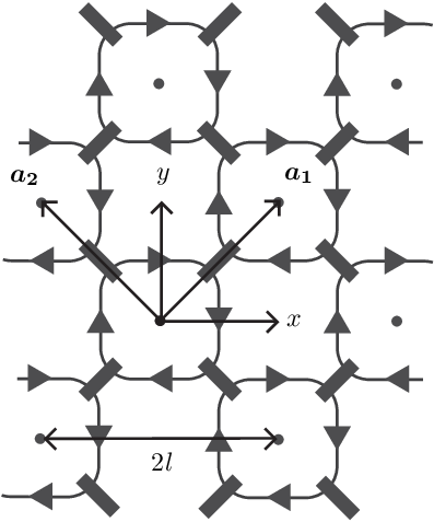
The Chalker-Coddington network model [7, 9] was originally introduced in order to analyze the localization transition in the quantum Hall effect. Our interest in this model stems from the fact that it is known to map onto the two-dimensional Dirac equation.[8] We briefly recall how the network model is defined and how the mapping to the Dirac equation works. We consider the square lattice shown in Fig. 2, with lattice constant and lattice vectors
| (22) |
The integers label the lattice site . With each site is associated a single current loop circling the site without enclosing any neighboring sites, say clockwise if viewed from the positive axis. The radii of these loops are expanded until states associated with nearest neighboring sites overlap. At these points of overlap, states on adjacent loops can scatter into each other.
As illustrated in Fig. 3, four current amplitudes , are associated with each site . These are amplitudes incident upon points of overlap, ordered clockwise, starting from the point of overlap with site . Each incident wave amplitude has picked up a phase since the previous point of overlap. With the point of overlap between loop and is associated a scattering matrix , while is associated with the point of overlap between and .

The matrix elements of and are arranged such that
Ho and Chalker[8] showed how this model can be mapped onto the Dirac equation for two-dimensional fermions. Firstly, one parametrizes the scattering matrices in terms of Pauli matrices ,
(The same matrix of coefficients is used for and .) For given fields , , and in the Dirac equation, the mapping then dictates a corresponding choice of parameters in the network model, namely and have to satisfy[8]
| (25a) | |||||
| (25b) | |||||
| (25c) | |||||
| (25d) | |||||
With this choice of parameters there is an approximate equality between a solution of the Dirac equation and the current amplitudes of the network model,
| (26) |
The accuracy of the approximation is improved by making the lattice constant smaller and smaller.
As mentioned in Sec. II, we will be considering two types of boundary conditions at and in the sample region . The periodic boundary condition is realized in the network model by putting the square lattice on a cylinder of circumference oriented along the -axis. The infinite-mass boundary condition is realized[8] by terminating the square lattice at and and adjusting the scattering phases along the edge. The edge lies at sites and the edge lies at sites . As shown in App. A, for sites Eq. (23) must be replaced with
| (27) |
while for sites it must be replaced with
| (28) |
IV Correspondence between scattering matrices of Dirac equation and network model
In this section we combine the known results summarized in the previous two sections to construct the scattering matrix of a graphene strip with heavily doped leads from a solution of the network model. This construction does not immediately follow from the correspondence (26) because the limit of heavily doped leads still needs to be taken. At first glance it would seem that, in order to preserve the correspondence between the network model and the Dirac equation, we must simultaneously take the limit so that remains small. (The correspondence between the network model and the Dirac equation is correct only to first order in this quantity.) This would imply that very large networks are required for an accurate representation of the graphene strip.
It turns out, however, that it is not necessary to model the heavily doped leads explicitly in the network model, as we now demonstrate. We define the real-space transfer matrix as the matrix that relates and at the right edge of the network to and at the left edge of the network. The left edge () lies at sites with . The right edge at lies at sites . The real-space transfer matrix relates
| (29) |
We define the Fourier transform
| (30) |
with .
In view of the relation (26) between the Dirac wave function and the network amplitudes , , the real space transfer matrix of the Dirac equation is related to by a unitary transformation,
| (31) |
We can now use the relation (20) between and the transfer matrix to obtain
| (32) |
where we have used
| (33) |
From Eq. (32) it follows that the lower right blocks of and are equal: . Substitution into the Landauer formula (15) gives
| (34) |
The Landauer formula applied to the network model thus gives the conductance of the corresponding graphene sheet connected to heavily doped leads. For later use, we note the current conservation relation for , which follows from Eqs. (14) and (32)
| (35) |
V Numerical Solution

In this section we test the accuracy and efficiency of the solution of a scattering problem in graphene by means of the network model. As explained in Sec. IV we need to calculate the real space transfer matrix through the weakly doped region. The conductance of the corresponding graphene sample then follows from Eq. (34).
We calculate the real-space transfer matrix recursively by adding slices to the network and multiplying the transfer matrices of individual slices. Since a multiplication of transfer matrices is numerically unstable we stabilize the algorithm as explained in App. B. We limit the numerical investigation in this section to the case , where only the electrostatic potential is non-zero.
We have found that the efficiency of the algorithm can be improved by using the fact that, according to Eq. (25), there is some arbitrariness in the choice of the phases . For and , one choice of the phases could be
| (36) |
Another choice is
| (37) |
The correspondence (26) between the network model and the Dirac equation holds for both choices of the phases, however the corrections for finite are smaller for choice (37). More precisely, as shown in App. C, if and are zero, the network model does not contain corrections to the Dirac equation of order .
Let us first consider the analytically solvable case of a clean graphene sheet that is obtained by setting in the weakly doped region. The Dirac equation gives transmission probabilities[12]
| (38a) | |||||
| (38b) | |||||
For periodic boundary conditions the transverse wave vector is discretized as with
In Fig. 4 we compare Eq. (38) to the results from the network model for periodic boundary conditions in the weakly doped region. The small parameter that controls the accuracy of the correspondence is . We find excellent agreement for a relatively large .

Fig. 5 shows the conductivity
| (39) |
at the Dirac point () as a function of the aspect ratio . We do the calculation both for periodic and infinite mass boundary conditions in the weakly doped region. (In the latter case with ) Again we see excellent agreement with the analytical results from the Dirac equation[12].
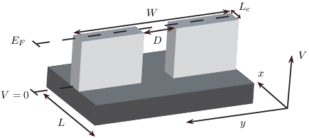
We now apply the network model to a case that cannot be solved analytically, because it involves inter-mode scattering. We take the electrostatic potential landscape shown in Fig. 6, which produces a narrow constriction or quantum point contact of width and length . In the weakly doped region, of length , electrons have an energy measured from the Dirac point. The barrier potential is tuned so that electron transport through the barrier takes place at the Dirac point, where all waves are evanescent. As the constriction is widened, the number of modes at a given energy that propagates through the opening increases. For fixed , this should lead to steps in the conductance as a function of opening width, at intervals of roughly . The steps are smooth because the current can also tunnel through the barrier.

We have calculated the conductance with the network model (solid curve in Fig. 7) and using the tight-binding model of graphene (dashed curve). In the tight-binding calculation we did not connect heavily doped leads to the weakly doped region. This does not affect the results, as long as .
Both calculations show a smooth sequence of steps in the conductance. The agreement is reasonably good, but not as good as in the previous cases. This can be understood since the tight-binding model of graphene is only equivalent to the Dirac equation on long length-scales.
The final numerical study that we report on in this paper involves transport at the Dirac point through a disordered potential landscape. Recent experimental studies[23] have observed electron and hole puddles in undoped graphene. The correlation length of the potential is larger than the lattice constant, hence intervalley scattering is weak. We are therefore in the regime of applicability of the network model (which eliminates intervalley scattering from the outset).

To model the electron and hole puddles, we devide the sample into an array of square tiles (Fig 8), where each tile has size , being the lattice constant of the network model. The electrostatic potential is constant on a single tile, but uncorrelated with the potential on the other tiles. We take the values of the potential on any given tile to be a random variable uniformly distributed between and . To make contact with previous studies[15, 16], we quantify the disorder strength by the dimensionless number
| (40) |
(The average is zero.) With tiles of dimension , the relation between and is and the network model faithfully represents the Dirac equation for values up to . We use a sample with aspect ratio and average over disorder realizations. We repeat the calculation for two different sample sizes namely and . The calculation is performed for transport at energy , i.e. the Dirac point of a clean, undoped sample.

In Fig. 9 we show the average conductance. Remakably enough the conductance increases with increasing disorder strength. This is consistent with the results obtained in Refs. 15, 16, 17, 18. The effect should not depend on the shape of the tiles in our model for the disorder. We have therefore repeated the calculation with rhombic instead of square tiles. We find deviations of less than .
The increase in conductance is explained by the non-zero density of states at the Dirac point that is induced by the disorder, together with the absence of back-scattering for Dirac electrons. While we do not make a detailed study of the dependence of conductance on sample size (at fixed aspect ratio), we note that the conductance of larger samples (squares in Fig. 9) is larger than the conductance of the smaller samples (circles in Fig. 9). This is consistent with the scaling behavior found in Refs. 16, 17, 18.
VI Conclusion
In conclusion, we have shown how the Chalker-Coddington network model can be used to solve a scattering problem in a weakly doped graphene sheet between heavily doped electron reservoirs (which model the metallic contacts). The method is particularly useful when the scattering problem does not allow an analytical solution, so that a numerical solution is required. The network model eliminates intervalley scattering from the outset. Thus, with a given mesh size, a larger graphene sample can be modeled with the network model than with methods based on the honeycomb lattice. The key technical result of our work is that an infinitely high potential step at the contacts can be implemented analytically by a unitary transformation of the real-space transfer matrix, without having to adjust the lattice constant of the network model to the small values needed to accommodate the small wave length in the contacts. We have demonstrated that the algorithm provides an accuracy and efficiency comparable to the tight-binding model on a honeycomb lattice. In agreement with the existing literature[15, 16, 17, 18] we have found that disorder that is smooth on the scale of the graphene lattice constant enhances conductivity at the Dirac point. The absence of intervalley scattering in the network model may prove useful for the study of these and other single-valley properties.
Acknowledgements.
This research was supported by the Dutch Science Foundation NWO/FOM and by the European Union’s Marie Curie Research Training Network (contract MRTN-CT-2003-504574, Fundamentals of Nano-electronics).Appendix A Infinite-mass boundary condition for the network model
In this appendix we consider the boundary condition imposed on the Dirac equation by termination of the network along a straight edge. We consider the eight orientations shown in Fig. 10 which have the shortest periodicity along the edge. Since we want to discuss the long wave-length limit, each edge needs to be much longer than the lattice constant . (In this respect the figure with its relatively short edges is only schematic.) The orientations are defined by the vector , , which is perpendicular to the edge and points outwards.
We wish to impose the infinite mass boundary condition[19]
| (41) | |||||
on the Dirac wavefunction at the edge. In view of the correspondence (26) between the Dirac equation and the network model, Eq. (41) implies the boundary condition
| (42) |
on the network amplitudes.

Away from the edge, the network amplitudes obey the equations (23). For , , , and all equal to zero (Dirac point) these reduce to
We can eliminate the amplitudes and to arrive at the equations
| (44a) | ||||
| (44b) | ||||
There are two linearly independent solutions and . When the network is truncated along an edge, the bulk equations (44) do not hold for the amplitudes along the edge. We seek the modified equations that impose the boundary condition (42) up to corrections of order .
The edge orientation was previously considered by Ho and Chalker[8]. We consider here all four independent orientations , , , and . The other four orientations , , , and are obtained by a symmetry relation.

Edge is constructed by removing all sites with . (See Fig. 11.) This means that the network amplitudes are prevented from scattering into the non-existent amplitudes belonging to the removed sites . Similarly, the amplitudes are prevented from scattering into the non-existent amplitudes . To do this one must modify the scattering matrices so that can only scatter into and so that can only scatter into . As a consequence, for Eq. (43) is replaced by
| (45) |
We eliminate and to arrive at Eq. (44) for and Eq. (44b) for . Eq. (44a) for is replaced by
| (46) |
The solution indeed satisfies the infinite mass boundary condition (42) with .

Edge is constructed by removing all sites with . (See Fig. 12.) This means that the network amplitudes are prevented from scattering into the non-existent amplitudes belonging to the removed sites . For , we replace Eq. (43) by
| (47) |
If we now eliminate the amplitudes and we find that Eq. (44) is still valid for all . For , Eq. (44b) still holds, while Eq. (44a) is changed to
| (48) |
The solution satisfies the infinite mass boundary condition (42) with .

Next, we consider edge , which results from the removal of all sites with . (See Fig. 13.) In this case, must be modified to prevent from scattering into . Furthermore, must be modified to prevent from scattering into . For we replace Eq. (43) by
| (49) |
and eliminate and to verify that the boundary condition holds.
The condition (49) modifies three of the equations (44):
| (50a) | |||||
| (50b) | |||||
| (50c) | |||||
For Eq. (44) holds without modification and Eq. (44b) also holds for . The solution
| (51) |
implies for , which satisfies the infinite mass boundary condition (42) with .

Edge results from the removal of all sites with . (See Fig. 14.) We must modify such that does not scatter into . To do this we replace Eq. (43) for sites by
| (52) |
We again eliminate and to arrive at
while for Eq. (44) still holds. The solution obeys the infinite mass boundary condition (42) with , as required.
This completes the boundary conditions for the four orientations , , , and . The orientations , , , and are obtained by the following symmetry: The network model is left invariant by a rotation in coordinate space (which takes to ) together with the application of in spinor space (which takes to and to ).
Appendix B Stable method of multiplication of transfer matrices
To construct the transfer matrix of a conductor one can divide it into slices, compute the transfer matrix of each slice, and multiply the individual transfer matrices. This recursive construction is numerically unstable, because products of transfer matrices contain exponentially growing eigenvalues which overwhelm the small eigenvalues relevant for transport properties. Chalker and Coddington [7] used an orthogonalisation method [20, 21] to calculate the small eigenvalues in a numerically stable way. To obtain both eigenvalues and eigenfunctions we employ an alternative method [22, 16]: Using the condition of current conservation, the product of transfer matrices can be converted into a composition of unitary matrices, involving only eigenvalues of unit absolute value.
We briefly outline how the method works for the real space transfer matrices of the network model, defined by Eq. (29). For the recursive construction it is convenient to rewrite this definition as
| (54) |
The numbers are integers, so that is the transfer matrix from to . The composition law for transfer matrices is matrix multiplication,
| (55) |
with initial condition identity matrix.
The unstable matrix multiplication may be stabilized with the help of the condition of current conservation (see Sec. IV). Because of this condition, the matrix constructed from by
| (56) |
is a unitary matrix (). Matrix multiplication of ’s induces a nonlinear composition of ’s,
| (57) |
defined by
| (58) |
| (59a) | |||||
| (59b) | |||||
| (59c) | |||||
| (59d) | |||||
The algorithm now works as follows: Multiply a number of transfer matrices and stop well before numerical overflow would occur. Transform this transfer matrix into a unitary matrix according to Eq. (56). Continue with the next sequence of transfer matrices, convert to a unitary matrix and convolute with the previous unitary matrix. At the end, we may transform back from to by the inverse of relation (56)
| (60) |
In practice this final transformation is unnecessary. According to Eq. (56) the upper-right block of is , which is all we need to calculate the conductance using the Landauer formula (34).
Appendix C Optimal choice of phases in the network model
In Sec. V we noted that the same long-wavelength correspondence between the Dirac equation and the network model can be obtained for different choices of the phases . Among these choices, the choice (37) avoids corrections of order to the Dirac equation. Here we show why.
For Eq. (25) reduces to
| (61a) | ||||
| (61b) | ||||
| (61c) | ||||
where we have defined the dimensionless quantity . The parameter can be chosen arbitrarily. We wish to show that the choice is optimal. We substitute Eq. () into Eq. () of Sec. III, with this parametrization, and obtain
| (62a) | ||||
| (62b) | ||||
Now we expand in , keeping terms to first order, and take and to be functions defined for all and smooth on the scale of the lattice. From Eq. (62) we then obtain
After transforming to , with as in Eq. (26), the first term on the r.h.s. of Eq. (C) becomes the desired Dirac equation. If we choose then the potential has to be smooth on the scale of the lattice, for the second term to be negligible in comparison with the first. We conclude that is the optimal choice.
References
- [1] A. H. Castro Neto, F. Guinea, N. M. R. Peres, K. S. Novoselov, and A. K. Geim, arXiv:0709.1163.
- [2] J. W. McClure, Phys. Rev. 104, 666 (1956).
- [3] M. P. A. Fisher and E. Fradkin, Nucl. Phys. B 251, 457 (1985).
- [4] A. W. W. Ludwig, M. P. A. Fisher, R. Shankar, and G. Grinstein, Phys. Rev. B 50, 7526 (1994).
- [5] D.-H. Lee, Phys. Rev. B 50, 10788 (1994).
- [6] K. Ziegler, Europhys. Lett. 31, 549 (1995).
- [7] J. T. Chalker and P. D. Coddingon, J. Phys. C 21, 2665 (1988).
- [8] C.-M. Ho and J. T. Chalker, Phys. Rev. B 54, 8708 (1996).
- [9] B. Kramer, T. Ohtsuki, and S. Kettemann, Phys. Rep. 417, 211 (2005).
- [10] A. K. Geim and K. S. Novoselov, Nature Mat. 6, 183 (2007).
- [11] K. Hirose, T. Ohtsuki, and K. Slevin, Physica E 40, 1677 (2008).
- [12] J. Tworzydło, B. Trauzettel, M. Titov, A. Rycerz, and C. W. J. Beenakker, Phys. Rev. Lett 96, 246802 (2006).
- [13] H. Schomerus, Phys. Rev. B 76, 045433 (2007).
- [14] Ya. M. Blanter and I. Martin, Phys. Rev. B 76, 155433 (2007).
- [15] A. Rycerz, J. Tworzydło, and C. W. J. Beenakker, Europhys. Lett. 79, 57003 (2007).
- [16] J. H. Bardarson, J. Tworzydło, P. W. Brouwer, and C. W. J. Beenakker, Phys. Rev. Lett. 99 106801 (2007).
- [17] K. Nomura, M. Koshino, and S. Ryu, Phys. Ref. Lett. 99, 146806 (2007).
- [18] P. San-Jose, E. Prada, and D. Golubev, Phys. Rev. B 76, 195445 (2007).
- [19] M. V. Berry and R. J. Mondragon, Proc. R. Soc. Lond. A 412, 53 (1987).
- [20] J. L. Pichard and G. Sarma, J. Phys. C 14, L127 (1981).
- [21] A. MacKinnon and B. Kramer, Z. Phys. B 53, 1 (1983).
- [22] H. Tamura and T. Ando, Phys. Rev. B 44, 1792 (1991).
- [23] J. Martin, N. Akerman, G. Ulbricht, T. Lohmann, K. von Klitzing, and A. Yacoby, Nature Physics 4, 144 (2008).