Heat Conduction Process on Community Networks as a Recommendation Model
Abstract
Using heat conduction mechanism on a social network we develop a systematic method to predict missing values as recommendations. This method can treat very large matrices that are typical of internet communities. In particular, with an innovative, exact formulation that accommodates arbitrary boundary condition, our method is easy to use in real applications. The performance is assessed by comparing with traditional recommendation methods using real data.
pacs
44.10.+i, 89.70.+c, 89.20.HhWith the advent of the internet, there sprout many web sites that enable large communities to aggregate and interact. For example livejournal.com allows its 3 million members to share interests and life experiences; del.icio.us is a social bookmark service for people to share their findings on the World Wide Web. Thousands of such web sites are built by web entrepreneurs and activists for the public, and their number is growing ever faster. This brings about massive amount of accessible information, more than each individual is able or willing to process. Information search, filtering, and recommendation thus become indispensable in internet era. Ideally speaking, a good recommendation mechanism should be able to “guess” what a person may want to select based on what he or she already selected [1, 2]. Many such mechanisms are in actual use (like www.amazon.com proposing its readers with new books), however, jury is still out as to what is the best model. For a review of current techniques, see [3].
Based on the heat conduction (or diffusion) process, we propose a recommendation model capable of handling individualized boundary conditions (BC). To better explain our model, we first illustrate using the friendship network of people: each person (member) is a node, and a pair of nodes is connected by an edge provided they are mutual friends. The collection of these information forms the symmetric adjacency matrix : element , or depending on whether people and are mutual friends (1) or not (0). Although it is possible to consider asymmetric connection, this generalization will not be studied here. To recommend friends to any individual member, we first set (Dirichlet) BC: to set the values on the directly connected nodes as 1 and some remote nodes (will be further specified) as 0. Values on all other nodes are treated as variables to be determined. These values can be interpreted as the probabilities that these nodes might be selected as friends.
We now describe an efficient and effective strategy to solve the proposed heat conduction problem. From , we first construct a propagator matrix , where is the diagonal degree matrix. Denote as the temperature vector of components: the source-components are high temperature nodes with temperature ; the sink-components are low temperature nodes with temperature . Our task is to find, through thermal equilibrium, the temperatures associated with the remaining nodes that are neither sinks nor sources. The discrete Laplace operator, analog of , on this network is , where is the identity matrix. We only need to solve
| (1) |
where is the external flux vector. Note that this is the discrete analog of with plays the role of and plays the role of .
Because Laplace operator conserves total heat and tend to spread heat from high temperature region to low temperature region, the only way to maintain the fixed temperature values at the sources and sinks is to apply external heat flux (inflow at sources and outflow at sinks). For the rest of the nodes, the equilibrium condition demands that no net heat flux should occur. Therefore, the only allowed nonzero components of are source- and sink-components.
The computation of the temperature vector is straightforward. It is convenient to group the source and sink components together into a block , and the rest free variables another block . That is
| (2) |
Likewise, we group the Laplace operator in a similar fashion and eq. (1) may be expressed as
| (3) |
All we need to solve is the homogeneous equation
| (4) |
without the need to know . Fixing the values of , can be readily found using standard iterative methods [4]. The above approach, although straightforward, represents a daunting challenge: for each individual, we must solve the huge matrix problem once – a prohibitively expensive task for a typical internet community having millions of members.
The standard way to get around this dilemma is to resort to the Green’s function method. Starting from eq.(1) we would like to have a Green’s function such that eq.(1) can be inverted:
| (5) |
to get . However, is divergent: the Laplace operator has a zero eigenvalue and the inverse is meaningful only if is in the subspace that is orthogonal to the eigenvector of zero eigenvalue. A fortunate scenario like this has occurred in the studies of random resistor networks [5, 6].
To simultaneously deal with all possible BC, we lose the freedom to limit the solution to a certain subspace. Nevertheless, we have a good understanding regarding this divergence. Basically, the matrix has an eigenvalue one with the right eigenvector being a column of s
and with left eigenvector being
where denotes the degree of node and being the sum of degrees. Note that with this notation, we have .
We may then decompose into
with . Further, the spectral radius of is now guaranteed to be smaller than and thus is invertible with . We may then rewrite the eq.(3) as
where the -dependent constant may be written as . We need to explain the notation further. Basically , represents a column vector whose components are obtained from the column vector with component labels corresponding to that of the sources and the sinks. On the other hand, represents a column vector that is the remainder of after removing the components whose labels correspond to the sources and sinks. Similarly, we define to be a row vector whose components are obtained from the row vector with component labels corresponding to that of the sources and the sinks; while represents a row vector that is the remainder of after removing the components whose labels correspond to the sources and sinks. To simplify the notation, we will represent by without explicitly showing its dependence.
Note that since , upon multiplying to both side of eq.(Heat Conduction Process on Community Networks as a Recommendation Model) we have
| (16) |
or equivalently
| (17) |
Consequently, we may write in the following form
| (18) |
Using the definition that , we obtain
or equivalently
| (19) |
Substituting this result back to eq. (18), we obtain with computational complexity solely depending on . Note that we only needs to invert the matrix once and for all. Upon specifying the boundary nodes, one needs to reshuffle the rows and columns of the matrix as well as vectors – a relatively efficient operation. This operation groups the source nodes and sink nodes in one block to make easy the computation of .
Let us emphasize that our final expression is written in a rather general setting that it can be applied to cases when is either row-normalized or column-normalized. In the case of column-normalized , we will have and . The solution structures (18-19), however, does not change.
Although an exact Green’s function method with Dirichlet boundary condition using spectral analysis (eigenvalues and eigenvectors) has been established by Chung and Yau [7], we find our method more convenient for computational purpose. With our method, the Greens function is computed once and can be used for all different BC. This is immensely more efficient than finding all the eigenvalues and eigenvectors for every BC needed for each individual. Furthermore, it would not be practical to find all the eigenvectors of matrices resulting from networks of millions of nodes.
To apply our method, one may either choose to fully invert or take its approximate form. The direct inversion of may still be computationally challenging for a matrix of size millions by millions. In terms of approximations, we find the use of particularly useful, with
| (20) |
This approximation gets better for larger . This is because the larger is, the smaller the difference between and . One may then use in place of . The quality of this approximation may be be verified comparing the two models: the exact solution(18-19) versus the approximate one (ie. replacing by in the exact solution).
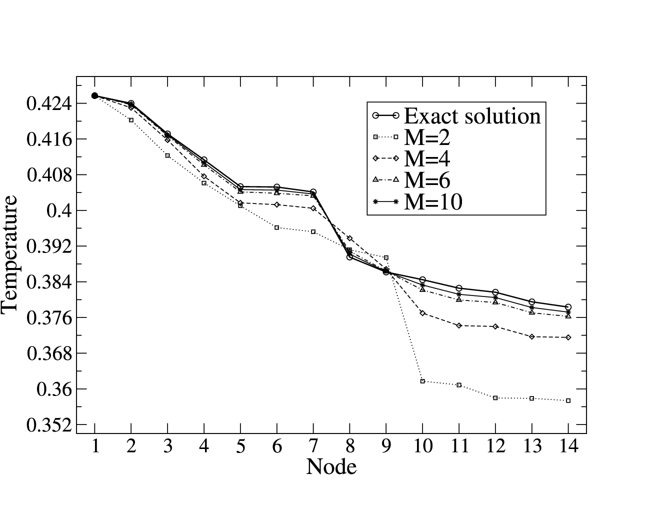
The convergence of the approximate solution to the exact solution (eqs.(18-19)) was first tested on an artificially generated random network of nodes. Aside from the condition that the nodes do not form disjoint clusters, a pair of nodes has probability to be connected. One then randomly selects a sink node and a source node that are not directly linked. We expect to get very similar shape of the temperature-profile as in the exact case. This is because for the row-normalized matrix, the vector being a column vector with in each entry may induce a small but uniform offset in the approximate solution. In Fig. 1, we plot the “temperature-profile” of the hottest nodes from the exact solution and the “temperature-profile” of the same nodes using our approximation solution of various . A good agreement between the exact solution and the approximate solution is reached at about .
To test the usability of our approach in real world, we use the movielens database. MovieLens (movielens.umn.edu; grouplens.org) ratings are recorded on a five stars scale and contain additional information, such as the time at which an evaluation was made. The data set we downloaded contains users movies. However, only a fraction of all possible votes were actually expressed. To be able to perform the calculation in reasonable time, we decide to further reduce the data size in each dimension by roughly %. To preserve the statistical properties of the original data, the pruning is done randomly without bias. In particular, we tried to maintain the probability distribution of the number of votes per users, as well as the sparsity and the ratio. We want to stress that this is crucial when testing the performance of predictive algorithms on real data in an objective way. In fact, many recommender systems can be found in the literature that rely on dense voting matrices [8, 9], at least in the traning data set. Typically, users who have judged too few items are struck out, as well as items that have received too few votes. We did not comply to such convention and made an effort to keep the filtering level as low as possible, although this makes predictions much more difficult.

Once filtered, we cast the data set in a vote matrix , with number of users and number of movies . In this reduced vote matrix, the matrix element represents the number of stars assigned to movie by user and is set to zero for unexpressed votes. The total filling fraction of is . The votes in are then sorted according to their relative timestamps. The last expressed votes are collected to form our test set, while the rest of the expressed votes form our training set. We denote by the vote matrix information up to time . That is, in all the unexpressed votes up to time are set to have zero star.
For the purpose of rating prediction, one will need a movie – movie network. To accomplish this task, one may compute the correlation coefficient between movie and movie using the expressed votes up to a certain time in the training set. Specifically, we denote and . The correlation coefficient reads
| (21) |
With a specified cutoff , one obtains an adjacency matrix , with . The value of is set so that the average degree per node for the movie – movie network has the same number of non-zero entries as .
Keeping the test set data fixed, we progressively fill the vote matrix the training set data over time (using the relative time stamps), say up to time . We then use to construct the the propagator based on the information accumulated up to . For each viewer (user), the BC is simply given by the votes expressed by the user up to time . In the event that a user only has one vote (or none) up to time , the BC for that user is given by randomly choosing one (or two) movie(s) and use the average rating(s) of the movie(s) up to that time as the boundary values [11]. We then use our algorithm to make predictions on the entire test set.
This test protocol is intended to reproduce real application tasks, where one aims to predict future votes –which is, of course, much harder than predicting randomly picked evaluations. It is somewhat less realistic to fix the test set once and for all, but this has the advantage to allow for more objective comparisons of the results. Many different accuracy metrics have been proposed to assess the quality of recommendations (see ref. [12]), we choose the Root Square Mean Error:
| (22) |
where represents the predicted vote from our algorithm, represents the actual vote (rated by user on movie ) in the test set, and the sum runs over all expressed votes in the test set. In our experiments, the RSME is calculated, at different sparsity values , on a unique test set.
Fig. 2 summarizes the performance comparison of our model with the mean predictor (the prediction is simply given by the objects mean value) and the widely used Pearson correlation based method [13, 14]. Our model outperforms both after enough votes (of the order of ) have been expressed. Since the dimensions of the vote matrix is known in a real application, given the number of expressed votes, it is relatively easy to see where one stands in terms of information content and whether our method will perform well using the given partial information.
In summary, we have devised a recommendation mechanism using analog to heat conduction. The innovation of our method is its capability to compute the Green’s function needed just once to accommodate all possible BC. In terms of generalization, it is apparent that our method can be applied to network with weighted edges, with . Whether such a generalization will improve the performance will be investigated in a separate publication. Finally, we stress that our study is not aimed to extract statistical properties out of networks through constructing model networks mimicking the real world networks [15, 16]; nor are we pursuing analysis of slowly decaying eigenmodes [17] in the absence of boundary condtitions. Instead, our goal is to provide a framework that is capable of providing individualized information extraction from a real world network.
YCZ and MB were partially supported by Swiss National Science Foundation grant 205120-113842. YCZ acknowledges hospitality at Management School, UESTC, China, where part of the work is done. The research of YKY was supported by the Intramural Research Program of the National Library of Medicine at the NIH.
References
- [1] S. Maslov and Y.C. Zhang, Phys. Rev. Lett. 87, 248701 (2001).
- [2] M. Blattner, Y.C. Zhang, and S. Maslov, Physica A 373, 753 (2006).
- [3] G. Adomavicius and A. Tuzhilin, IEEE Transactions on Knowledge and Data Engineering 17, 734 (2005), ISSN 1041-4347.
- [4] W. Press, S. Teukolsky, B. Flannery, and V. Vetterling, Numerical Recipes in C (Cambridge University Press, New York, USA, 1992).
- [5] G. Korniss, M. Hastings, K. Bassler, M. Berryman, B. Kozma, and D. Abbott, Phys. Lett. A 350, 324 (2006), ISSN 1046-8188.
- [6] F. Wu, J. Phys. A 37, 6653 (2004).
- [7] F. Chung and S. Yau, Journal of Combinatorial Theory(A) pp. 141–214 (2000).
- [8] K. Goldberg, T. Roeder, D. Guptra, and C. Perkins, Information Retrieval 4, 133 (2001).
- [9] A. Waern, User Modeling and User-Adapted Interaction 14, 201 (2004).
- [10] Assuming that the vote matrix is filled randomly, one can show that the density needs to be to have in the movie–movie network a linking probability , which marks the onset of giant cluster formation. See B. Bollobás, Random Graphs, chap. 6 (Cambridge University Press, New York, USA, 2001).
- [11] This is to avoid the artifact of null information retrieval: e.g. assume only one boundary node with a specified temperature, all nodes will reach the same temperature upon thermal equilibrium.
- [12] J. Herlocker, J. Konstan, L. Terveen, and J. Riedl, ACM Trans. Inf. Syst. 22, 5 (2004), ISSN 1046-8188.
- [13] P. Resnick, N. Iacovou, M. Suchak, P. Bergstorm, and J. Riedl, in Proceedings of ACM 1994 Conference on Computer Supported Cooperative Work (ACM, Chapel Hill, North Carolina, 1994), pp. 175–186.
- [14] J. Herlocker, J. Konstan, and J. Riedl, in Computer Supported Cooperative Work (2000), pp. 241–250.
- [15] M. Newman, SIAM Review 45, 167 (2003c).
- [16] J. Park and M. Newman, Phys. Rev. E 70, 066117 (2004).
- [17] K. A. Eriksen, I. Simonsen, S. Maslov, and K. Sneppen, Phys. Rev. Lett. 90, 148701 (2003).