Local Approximation Schemes for Topology Control
Abstract
This paper presents a distributed algorithm on wireless ad-hoc networks that runs in polylogarithmic number of rounds in the size of the network and constructs a linear size, lightweight, -spanner for any given . A wireless network is modeled by a -dimensional -quasi unit ball graph (-UBG), which is a higher dimensional generalization of the standard unit disk graph (UDG) model. The -dimensional -UBG model goes beyond the unrealistic “flat world” assumption of UDGs and also takes into account transmission errors, fading signal strength, and physical obstructions. The main result in the paper is this: for any fixed , , and there is a distributed algorithm running in communication rounds on an -node, -dimensional -UBG that computes a -spanner of with maximum degree and total weight . This result is motivated by the topology control problem in wireless ad-hoc networks and improves on existing topology control algorithms along several dimensions. The technical contributions of the paper include a new, sequential, greedy algorithm with relaxed edge ordering and lazy updating, and clustering techniques for filtering out unnecessary edges.
Categories and Subject Descriptors: C.2.4 [Computer-Communication Networks]: Distributed Systems
General Terms: Algorithms, Performance, Theory.
Keywords: Spanners, Topology control, Wireless ad-hoc networks, Unit ball graphs.
1 Introduction
Let be a graph with edge weights . For , a -spanner of is a spanning subgraph of such that for all pairs of vertices , the length of a shortest -path in is at most times the length of a shortest -path in . The problem of constructing a sparse -spanner, for small , of a given graph has been extensively studied by researchers in distributed computing and computational geometry and more recently by researchers in ad-hoc wireless networks. In this paper we present a fast distributed algorithm for constructing a linear size, lightweight -spanner of bounded degree for any given , on wireless networks. Below, we describe our result more precisely.
1.1 Network model
We model wireless networks using -dimensional quasi unit ball graphs. For any fixed , and integer , a -dimensional -quasi unit ball graph (-UBG, in short) is a graph whose vertex set can be placed in one-one correspondence with a set of points in the -dimensional Euclidean space and whose edge set satisfies the constraint: if then and if then . Here we use to denote the Euclidean distance between the points corresponding to vertices and . The -UBG model does not prescribe whether a pair of vertices whose distance is in the range are to be connected by an edge or not. This is an attempt to take into account transmission errors, fading signal strength, and physical obstructions. Our algorithm does not need to know the locations of nodes of the -UBG in -dimensional Euclidean space; just the pairwise Euclidean distances.
The -UBG model is a higher dimensional generalization of the somewhat simplistic unit disk graph (UDG) model of wireless networks that is popular in literature. Specifically, when and , a -dimensional -UBG is just a UDG. UDGs are attractive due to their mathematical simplicity, but have been deservedly criticized for being unrealistic models of wireless networks [10]. In our view, -dimensional -UBGs are a significant step towards a more realistic model of wireless networks. Two-dimensional -UBGs were proposed in [1] as a model of wireless ad-hoc networks with unstable transmission ranges and the difficulty of doing geometric routing in such networks was shown.
Our communication model is the standard synchronous message passing model that does not account for channel access and collision issues. In this communication model, time is divided into rounds. In each round, each node can send a different message to each of its neighbors, receive different messages from all neighbors and perform arbitrary (polynomial) local computation. The length of messages exchanged between nodes is logarithmic in the number of nodes. We measure the cost of our algorithm in terms of the number of communication rounds. Although this model is not widely considered to be realistic, it is nevertheless interesting because it demonstrates the locality of computations.
1.2 Our result
For any edge weighted graph , we use to denote the sum of the weights of all the edges in and to denote a minimum weight spanning tree of . For any fixed , , and our algorithm runs in communication rounds on an -node, -dimensional -UBG and computes a -spanner of whose maximum degree and whose total weight . Since any spanner of has weight bounded below by , the weight of the output produced by the algorithm is within a constant times the optimal weight. As far as we know, our result significantly improves all known results of a similar kind along several dimensions. More on this further below.
1.3 Topology control
Our result is motivated by the topology control problem in wireless ad-hoc networks. For an overview of topology control, see the survey by Rajaraman [17]. Since an ad-hoc network does not come with fixed infrastructure, there is no topology to start with and informally speaking, the topology control problem is one of selecting neighbors for each node so that the resulting topology has a number of useful properties. More precisely, let be a set of nodes that can communicate via wireless radios and for each , let denote the set of all nodes that can reach when transmitting at maximum power. The induced digraph , where , represents the network in which every node has chosen to transmit at maximum power and has designated every node it can reach as its neighbor. The topology control problem is the problem of devising an efficient and local protocol for selecting a set of neighbors for each node . The induced digraph , where is typically required the satisfy properties such as symmetry (if then ), sparseness () or bounded degree ( for all nodes and some constant ), and the spanner property. Sometimes stronger versions of connectivity such as -vertex connectivity or -edge connectivity (for ) are desired, both for providing fault-tolerance and for improving throughput [6, 7]. If the input graph consists of nodes in the plane, it is quite common to require that the output graph be planar [13, 14, 15, 18, 19]. This requirement is motivated by the existence of simple, memory-less, geometric routing algorithms that guarantee message delivery only when the underlying graph is planar [9].
Though the topology control problem is recent, there is already an extensive body of literature on the problem to which the above sample of citations do not do justice. However, many of the topology control protocols that provide worst case guarantees on the quality of the topology, assume that the network is modeled by a UDG. A recent example [15] presents a distributed algorithm that requires a linear number of communication rounds in the worst case to compute a planar -spanner of a given UDG with and in which each node has degree at most 25. These two constants can be slightly tuned – can be brought down to about 3.8 with a significant increase in the degree bound. We improve on the result in [15] along several dimensions. As is generally known among practitioners in ad-hoc wireless networks, the “flat world” assumption and the identical transmission range assumption of UDGs are unrealistic [10]. By using an -UBG we significantly generalize our model of wireless networks, hopefully moving much closer to reality. For any , our algorithm returns a -spanner; as far as we know, this is the first distributed algorithm that produces an arbitrarily good spanner for an -UBG model of wireless networks. We also guarantee that the total weight of the output is within constant times optimal – a guarantee that is not provided in [15]. Finally, using algorithmic techniques and distributed data structures that might be of independent interest, we ensure that our protocol runs in communication rounds. We are not aware of any topology control algorithm that runs in poly-logarithmic number of rounds and provides anywhere close to the guarantees provided by our algorithm.
1.4 Spanners in computational geometry
Starting in the early 1990’s, researchers in computational geometry have attempted to find sparse, lightweight spanners for complete Euclidean graphs. Given a set of points in , the tuple , where is the set of line segments , is called the complete Euclidean graph on . For any subset , is called a Euclidean graph on . The specific problem that researchers in computational geometry have considered, is this. Given a set of points in and , compute a Euclidean graph on that is a -spanner of the complete Euclidean graph on , whose maximum degree is bounded by and whose weight is bounded by the weight of a minimum spanning tree on . For an early example, see [12] in which the authors show that there are “planar graphs almost as good as the complete graphs and almost as cheap as minimum spanning trees.” This was followed by a series of improvements [2, 3, 4, 5], with the most recent paper [2] presenting algorithms for constructing Euclidean subgraphs that provide the additional property of -fault tolerance. Most of the papers mentioned above start with the following simple, greedy algorithm.
Algorithm SEQ-GREEDY ()
1. Order the edges in in non-decreasing order of length.
2. ,
3. For each edge if there is no -path in of length at most
- (a)
- (b)
Output .
It is well-known [4] that if the input graph is the complete Euclidean graph, then the output graph produced by SEQ-GREEDY has the following useful properties: (i) is a -spanner of , (ii) , and (iii) . A naive implementation of SEQ-GREEDY takes time because a quadratic number of shortest path queries need to be answered on a dynamic graph with edges. Consequentially, papers in this area [4, 5] focus on trying to implement SEQ-GREEDY efficiently. For example, Das and Narasimhan [4] show how to use certain kind of graph clustering to answer shortest path queries efficiently, thereby reducing the running time of SEQ-GREEDY to . One of the contributions of this paper is to show how a variant of the Das-Narasimhan clustering scheme can be implemented and maintained efficiently, in a distributed setting.
1.5 Summary of our contributions
In obtaining the main result, our paper makes the following contributions.
- 1.
We first show that sparse, lightweight -spanners for arbitrarily small , not only exist for -dimensional -UBGs, but can be computed using SEQ-GREEDY. Note that sparse -spanners for arbitrarily small values of do not exist for general graphs. For example, there is a classical graph-theoretic result that shows that for any , there exist (infinitely many) unweighted -vertex graphs for which every -spanner needs edges (see Page 179 in [16]).
- 2.
We then consider a version of SEQ-GREEDY in which the requirement that edges be considered in increasing order of length is relaxed. More precisely, the edges are distributed into bins such that edges in are all shorter than edges in . It is then shown that any ordering of the edges in which edges in come first, followed by edges in , followed by the edges in , etc., is good enough for the correctness of SEQ-GREEDY, even for -dimensional -UBGs. More importantly, we show that the update step in SEQ-GREEDY (Step 3(a)) need not be performed after each edge is queried. Instead, a more lazy update may be performed, after each bin is completely processed. Being able to perform a lazy update is critical for a distributed implementation; roughly speaking, we want the nodes to query all edges in a bin in parallel and not to have to rely on answers to queries on other edges in a bin.
- 3.
We also use a clustering technique as a way to reduce the number of edges to be queried per node. Reducing the number of query edges per node, is critical to being able to guarantee that the output of our distributed version of SEQ-GREEDY does not have too many edges incident on a node.
- 4.
Our next contribution is to show that this relaxed version of SEQ-GREEDY can be implemented in a distributed setting in phases — one phase corresponding to each bin — such that each phase requires communication rounds. Each phase requires the computation of maximal independent sets (MIS) on some derived graphs. We show that the derived graphs are unit ball graphs of constant doubling dimension [11] and use the -round MIS algorithm of Kuhn et al [11].
1.6 Extensions to our main result
Here we briefly report on extensions to our main result that we have obtained. They do not appear in this paper due to lack of space.
- 1.
Let be an edge-weighted graph. For any and positive integer , a -vertex fault-tolerant -spanner of is a spanning subgraph if for each subset of vertices of size at most , is a -spanner of . A -edge fault-tolerant -spanner is defined in a similar manner. Using ideas from [2] we can extend our algorithm to produce a -vertex (or a -edge) fault-tolerant -spanner in polylogarithmic number of communication rounds.
- 2.
In this paper, we use Euclidean distances as weights for the edges of the input graph . However, if the metric , for positive constant and , is used in place of Euclidean distances , we can show that our algorithm still produces a spanner with all three desired properties. Relative Euclidean distances, such as the function mentioned above, may be used to produce energy spanners.
- 3.
Let be an edge-weighted graph. The power cost of a vertex is . In other words, the power cost of a vertex is proportional to the cost of transmitting to a farthest neighbor. The power cost of is [8]. We can show that the output of our algorithm is not only lightweight with respect to the usual weight measure (sum of the weights of all edges) but also with respect to the power cost measure.
2 Sequential Relaxed Greedy Algorithm
Now we show that a relaxed version of SEQ-GREEDY produces an output with all three desired properties, even when the input is not a complete Euclidean graph, but is a -dimensional, -UBG for fixed and . Relaxing the requirement in SEQ-GREEDY that the edges be totally ordered by length and allowing for the output to be updated lazily are critical to obtaining a distributed algorithm that runs in polylogarithmic number of rounds.
Let be a constant to be fixed later and let for each . Let and for each let . Let . Then, since no edge has length greater than 1, the length of any edge in lies in one of the intervals . Let .
We now eliminate the restriction that edges within a set be processed in increasing order by length. We run SEQ-GREEDY in phases: in phase , the algorithm processes edges in in arbitrary order and adds a subset of edges in to the spanner. For , we use to denote the spanning subgraph of consisting of edges . Thus is the portion of the input graph that the algorithm has processed in phase and earlier. We use to denote the output of the algorithm at the end of phase . In other words, is the spanning subgraph of consisting of edges of that the algorithm has decided to retain in phases . The final output of the algorithm is .
The way is processed is different from the way , is processed. We now separately describe these two parts.
2.1 Processing Edges in
We start by stating a property of that follows easily from the fact that all edges in are small.
Lemma 1
Every connected component of induces a clique in .
The algorithm PROCESS-SHORT-EDGES for processing edges in consists of three steps (i) determine the connected components of , (ii) use SEQ-GREEDY to compute a -spanner for each connected component (that is, a clique), and (iii) let be the union of the -spanners computed in Step (2) and output . The following theorem states the correctness of the PROCESS-SHORT-EDGES algorithm. Its proof follows easily from the correctness of SEQ-GREEDY.
Theorem 2
satisfies the following properties. (i) For every edge , contains a -path of length at most , (ii) , and (iii) .
2.2 Processing Long Edges
We now describe how edges in are processed, for . The algorithm PROCESS-LONG-EDGES has five steps: (i) computing a cluster cover for , (ii) selecting query edges in , (iii) computing a cluster graph for , (iv) answering shortest path queries for the query edges selected in Step (ii), and (v) removing redundant edges. These steps are described in the next five subsections.
For any graph , let denote the vertex set for . For any pair of vertices let denote the length of a shortest -path in . Define a cluster of with center and radius to be a set of vertices such that, for each , . A set of clusters of is a cluster cover of of radius if every cluster in the set has radius , every vertex in belongs to at least one cluster, and for any pair of cluster centers and , .
2.2.1 Computing a Cluster Cover for
At the beginning of phase we compute a cluster cover of radius , where is a constant that will be fixed later. We start with an arbitrary vertex and run Dijkstra’s shortest path algorithm with source on , in order to identify nodes with the property that ; each such node gets included in the cluster . Once has been identified, recurse on until all nodes belong to some cluster and we have a cluster cover of of radius .
2.2.2 Selecting Query Edges in
As defined earlier, edges in have weights in the interval , while the cluster cover for has radius , with . This implies that each edge in has endpoints in different clusters. Our goal is to select a unique query edge per pair of clusters. This will guarantee that there are a constant number of query edges incident on any node (see Lemma 4) and this fact will be critically used by the distributed version of our algorithm to guarantee the degree bound on the spanner that is constructed.
Let be a quantity that satisfies and . For any value , no matter how small, there always exists a that satisfies these restrictions. Define an edge to be a covered edge if there is a such that (i) , and or (ii) , and . Any edge in that is not covered is a candidate query edge. The motivation for these definitions is the following geometric lemma, due to Czumaj and Zhao [2].
Lemma 3 (Czumaj and Zhao [2])
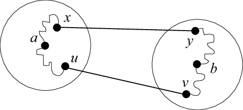
Let and . Let be three points in with . Suppose further that . Then the edge followed by a -spanner path from to is a -spanner path from to (see Figure 1).

Now note that for each covered edge , there exists that satisfies the preconditions of Lemma 3 (by definition), and using this lemma we can show that already contains a -path of length at most . This suggests that covered edges need not be queried and therefore we can start with the complement of the set of covered edges as candidate query edges.
For each pair of clusters and , let denote the subset of candidate query edges in with one endpoint in and the other endpoint in . Our algorithm selects a unique query edge from each nonempty subset . Assuming that and , the edge is selected so as to minimize
| (1) |
The quantity in (1) is carefully chosen to guarantee that, if a -spanner path between the endpoints of an edge that minimizes (1) exists in , then -spanner paths between the endpoints of all edges in exist in (this property will later be shown in the proof of Theorem 10). This implies that, for each pair of clusters and , querying the edge in that minimizes (1) renders querying any other edge in redundant.
The following lemma shows that selecting query edges as described above filters all but a constant number of edges per cluster. The proof follows from two observations: (i) if a pair of cluster centers are connected by an edge in , then the clusters are not too far from each other in Euclidean space (in particular, no farther than ), and (ii) the Euclidean distance between any pair of cluster centers is bounded from below by , because they would otherwise be part of the same cluster.
Lemma 4
The number of query edges in that are incident on any cluster is , a constant.
2.2.3 Computing a Cluster Graph
For each selected query edge , we need to know if contains an -path of length at most . In general, the number of hops in a shortest -path in can be quite large and having to traverse such a path would mean that the shortest path query corresponding to edge could not be answered quickly enough. To get around this problem, we use an idea from [4] in which the authors construct an approximation to , called a cluster graph, and show that for any edge , the shortest path query for can be answered approximately on in a constant number of steps. The goal of Das and Narasimhan [4] was to improve the running time of SEQ-GREEDY on complete Euclidean graphs, but we show that the Das-Narasimhan data structure can be constructed and maintained in a distributed fashion for efficiently answering shortest path queries for edges belonging to a -UBG. In the following, we describe a sequential algorithm that starts with a cluster cover of of radius , and builds a cluster graph of . This algorithm is identical to the one in Das and Narasimhan [4] and is included mainly for completeness.
The vertex set of is and the edge set of contains two types of edges: intra-cluster edges and inter-cluster edges. An edge is an intra-cluster edge if is a cluster center and is node in . Inter-cluster edges are between cluster centers. An edge is an inter-cluster edge if and are cluster centers, and at least one of the following two conditions holds: (i) , or (ii) there is an edge in with one endpoint in and the other endpoint in . See Figure 2.

Regardless of the type of a cluster edge (inter- or intra-), the weight of is the value of . The following lemma follows easily from the definition of inter-cluster edges.
Lemma 5
For any inter-cluster edge in , we have that .
The above upper bound also implies that . Using this and arguments similar to those used for Lemma 4, we can show that the number of inter-cluster edges incident to a cluster center is , so we have the following lemma.
Lemma 6
The number of inter-cluster edges in incident to a cluster center is , a constant.
The main reason for constructing the cluster graph is that lengths of paths in are close to lengths of corresponding paths in and shortest path queries for edges in can be answered quickly in . The following lemma (whose proof appears in Das and Narasimhan [4]) shows that we can construct such that path lengths in approximate path lengths in to any desired extent, depending on the choice of .
Lemma 7
For any edge , if there is a path between and in of length , then there is a path between and in of length such that .
2.2.4 Answering Shortest Path Queries
For query edges , we are interested in knowing whether has an -path of length at most . We ask this question on the cluster graph . If contains an -path of length at most , we do not add to ; otherwise we do. If contains an -path of length at most , then so does (by Lemma 7, since ). Therefore, not adding to the spanner is not a dangerous choice. On the other hand, even if does not contain an -path of length at most , might contain such a path and in this case adding edge is unnecessary. Adding extra edges is of course not problematic for the -spanner property. It will turn out that this is not a problem even for the requirement that the spanner should have bounded degree and small weight, given that paths in can approximate paths in to an arbitrary degree.
Given the structure of the cluster graph, all but at most 2 edges in any simple -path are inter-cluster edges. Since the radius of each cluster is , each inter-cluster edge has weight greater than . We are looking for a path of length at most . Since , we are looking for a path of length at most . Any simple path in of length at most has at most 2 + hops, which is a constant. This yields the following lemma.
Lemma 8
For any edge , if , then contains a shortest -path with hops (no more than 2 + ).
One issue we need to deal with, especially when attempting to construct and answer queries in in a distributed setting, is that edges in need not be present in the underlying network . Specifically, for an intra-cluster edge , where is a cluster and , it may be the case that and may be absent from . Similarly, an inter-cluster edge in may be absent in . However, for any edge in (intra- or inter-cluster edge), we have the bound . This follows from Lemma 5 and the fact that the radius of each cluster is . Thus a shortest -path in lies entirely in a ball of radius centered at . Since is a spanning subgraph of , this implies that there is a shortest -path in that lies entirely in the -dimensional ball of radius centered at . Since any two vertices in that are two hops away from each other are at least apart (in the -dimensional Euclidean space), contains at most hops. This argument yields the following theorem.
Theorem 9
For any edge , if , then contains a shortest -path with hops (no more than ).
This theorem implies that brute force search initiated from one of the endpoints, say , will be able to answer the shortest path query on edge in rounds in a distributed setting.
2.2.5 Removing Redundant Edges
Let be such that . Recall that shortest path queries for edges in are answered on , and so updates to in phase do not influence subsequent shortest path queries in phase . Thus it is possible that in phase two edges and get added to , yet both of the following hold:
- (i)
- (ii)
Note that, since holds for any pair of nodes and , and since , conditions (i) and (ii) above imply that contains -spanner paths from to and from to . We call two edges and satisfying conditions (i) and (ii) above mutually redundant: one of them could potentially be eliminated from , without compromising the -spanner property of . In fact, such mutually redundant pairs of edges need to be eliminated from because our proof that has small weight (Theorem 2.15) depends on the absence of such pairs of edges.
To do this, we build a graph that has a node for each edge in a mutually redundant pair and an edge between every pair of nodes that correspond to a mutually redundant pair of edges in . We construct an MIS of and eliminate from all edges associated with nodes in that do not appear in .
2.3 The Three Desired Properties
Let be the spanner at the end of phase . We now prove that satisfies the three properties that the output of SEQ-GREEDY was guaranteed to have. The proofs of these theorems form the technical core of the paper and are presented next in this section.
Theorem 10
For any , the output is a -spanner.
Proof 2.11.
We first prove that the theorem holds for all query edges in , then we extend the argument to non-query edges as well. Let be an arbitrary query edge and let be such that . Then either (i) is added to the spanner in phase , or (ii) . If the former is true and is not a redundant edge, then the theorem holds. If is a redundant edge but does not get removed from , then again the theorem holds. If is a redundant edge that gets removed from , then at least one mutually redundant counterpart edge must remain in (since removed edges form an independent set), ensuring a -spanner -path in . If (ii) is true, then from Lemma 7, (first part of the inequality) and therefore .
For non-query edges, the proof is by induction on the length of edges in . The base case corresponds to edges in , for which SEQ-GREEDY ensures that the theorem holds.
Assume that the theorem is true for any edge in of length no greater than some value , and consider a smallest non-query edge in of length greater than . We prove that . Let be such that . We now consider two cases, depending on whether is a candidate query edge in phase or not.
If is not a candidate query edge, then it is a covered edge. That is, there exists an edge in such that and , or an edge in such that and . The two cases are symmetric and so without loss of generality, assume that the former is true. Here satisfies the hypothesis of the Czumaj-Zhao lemma (Lemma 3), that is, and . Since and is an -UBG, this implies that is an edge is . Furthermore, since , we have . Refer to Figure 3a. If is a query edge, then by the argument above we have that contains a -spanner -path . Otherwise, if is not a query edge, since its length is less than the length of , by the inductive hypothesis we get that there is a -spanner -path . In either case, Lemma 3 tells us that followed by is a -spanner path from to , completing this case.
 |
 |
|---|---|
| (a) | (b) |
We now consider the case when is a candidate query edge in phase , but not a query edge. Let and be such that and , and let be the query edge selected in phase , with and . Refer to Figure 3b. Due to the criteria for selecting , we have
| (2) |
Recall that is the partial spanner at the end of phase . We show that . We discuss two cases, depending on whether was added to or not.
Assume first that was not added to . This means that . Note however that
| (3) | |||||
We now evaluate
This latter inequality involves simple substitutions that use inequalities (2) and (3), and completes this case.
Now assume that was added to . Since and has radius , we have that . Similarly, . These together with (2) yield
| (4) |
If the edge turns out to be redundant and eliminated from , the existence of a mutually redundant counterpart edge in ensures that . This enables us to construct in a path from to of weight
| (5) | |||||
since , and same for . We can now construct a path in from to of weight
Theorem 2.12.
has degree.
Proof 2.13.
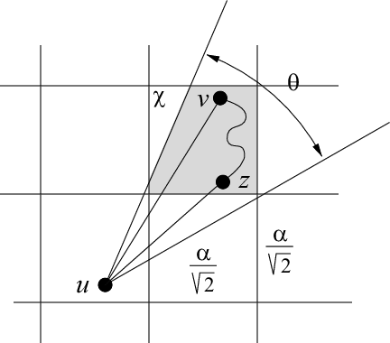
Let be a quantity satisfying the conditions of Lemma 3. Fix a vertex and consider the -dimensional unit radius ball centered at . For some that depends only on and , this ball can be partitioned into cones, each with apex , such that for any , in a cone, . Yao [20] shows how to construct such a partition with cones. Place an infinite axis-parallel grid of -dimensional cubes, each of dimension , on the plane. See Figure 4(c) for a 2-dimensional version of this picture. There are cells that intersect the unit ball centered at , and therefore there are cells that intersect each cone in the cone partition of this unit ball. Thus the cones and the square cells together partition the unit ball centered at into regions. We show that in , has neighbors in each region, which is a constant.
Let be neighbors of in that lie in a region . Without loss of generality, assume that , for , and let be such that . Since , we have that for all , , with .
We now prove that is in fact in for all . To derive a contradiction, assume that there is a such that , with . This means that just before edge is processed, contains edge . Also note that since and lie in the same region, . But, this means that is a covered edge in phase and will not be queried. This contradicts the presence of edge in .
We have shown that for all . Recall that our algorithm picks a unique query edge per pair of clusters. This along with Lemma 4 proves that is constant.
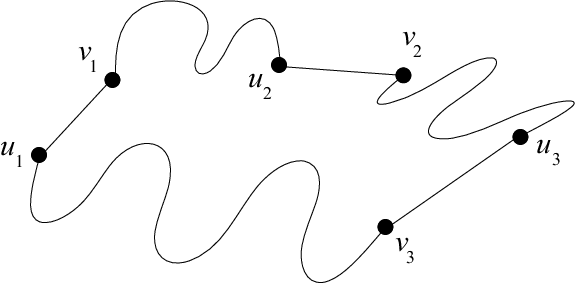
In the next theorem, we show that the spanner produced by the algorithm has small weight. The proof relies on the line segments in the spanner satisfying a property known as the leapfrog property [2, 5]. For any , a set of line segments, denoted , has the -leapfrog property if for every subset of
| (6) |
Informally, this definition says that if there exists an edge between and , then any path not including must have length greater than (see Figure 4(c) for an illustration of this definition). The following implication of the -leapfrog property was shown by Das and Narasimhan [4].
Lemma 2.14.
Let . If the line segments in -dimensional space satisfy the -leapfrog property, then , where is a minimum spanning tree connecting the endpoints of line segments in . The constant in the asymptotic notation depends on , and .
Theorem 2.15.
Let . Let denote . Let . When the relaxed greedy algorithm is run with these values of and , the output satisfies .
Proof 2.16.
Let be a constant picked as follows. When , pick satisfying . Otherwise, pick satisfying . Partition the edges of into subsets such that and for each , . Let . Then every edge in is in some subset , . We will now show that each satisfies the -leapfrog property, for any satisfying:
| (7) |
It is easy to check that our choice for , , and guarantee that each quantity inside the min operator is strictly greater than 1. Showing the -leapfrog property for would imply that , and since the edges of are partitioned into a constant number of subsets , .
Consider an arbitrary subset . To prove inequality (6) for , it suffices to consider the case when is a longest edge in . We consider separately from , .
The case. If for any , or , then the leapfrog property holds. So we assume that for all , and . Let be the phase in which gets processed, i.e., . Since , it is the case that for all , and . Hence, is a subset of edges of and each edge in this set gets processed in phase or earlier.
Assume first that at least one edge in the set gets processed in phase . Then the right hand side of inequality (6) is at least , since edges in have weights in the interval . Also since , and since the inequality is guaranteed by the values of and in (7), the leapfrog property holds for this case.
Assume now that all edges in have been processed in phase or earlier, meaning that -spanner paths between their endpoints exist in at the time gets processed. For , let be a shortest -path in , and let be a shortest -path in . Let be the following -path in : . Here, we use to denote concatenation. We distinguish three cases, depending on the size of the subset .
- (i)
. Then, . We also have that , since . It follows that for any . Furthermore, is no greater than the right hand side of the -leapfrog inequality (6), so lemma holds for this case as well.
- (ii)
. In addition to , assume that for some , . It the -leapfrog inequality (6) holds, we are done and so let us assume the opposite of that:
(8) Since all edges , , except for and are in , and since contains -spanner -paths for all , , and a -spannner -path, the above inequality yields
Multiplying both sides by and using (which is implied by our choice of ) and Lemma 7, we get
(9) Let . We now observe that
(10) implies the -leapfrog property. To see this use the fact that both and belong to and therefore , which substituted in (10) yields:
We get the lower bound on the left hand side of the above inequality by using again and our choice of . This yields the -leapfrog property. So we assume that inequality (10) does not hold, that is,
Since all edges , , except for and are in , and since contains -spanner -paths for all , , and a -spannner -path, the above inequality yields
Multiplying both sides by and using Lemma 7, we get
(11) Inequalities (9) and (11) imply that edges and are mutually redundant and therefore cannot both exist in the spanner — a contradiction.
- (iii)
. This means that exists in at the time is processed. Furthermore, , otherwise would not have been added to the spanner, a contradiction.
The case, . In this case, for all . If , then the right hand side of the -leapfrog inequality (6) is at least and therefore the -leapfrog inequality goes through for any . Otherwise, if , then we need to show that . If each of and is at most , then using the same argument as in the -case with , we can show that and are mutually redundant and will not both exist in the spanner. Otherwise, if one of or is greater than , then the right hand side of the -leapfrog inequality (6) is greater than . To ensure that the inequality goes through, we require that . Since , the above inequality is satisfied for any , which holds true cf. (7).
3 Distributed Relaxed Greedy Algorithm
We now describe a distributed version of the relaxed greedy algorithm from Section 2. Like the sequential relaxed greedy algorithm, this algorithm also runs in phases — with edges in being processed in phase . We will show that edges in can be processed in rounds. Recall that each subsequent phase consists of the following five steps: (i) computing a cluster cover of , (ii) selecting query edges in , (iii) computing a cluster graph of , (iv) answering shortest path queries for selected query edges, and (v) deleting some redundant edges. We will show that Steps (ii), (iii), and (iv) can be completed in rounds and Steps (i) and (v) take rounds. Step (i) and Step (v) will each involve computing an MIS in a certain derived graph and in both cases, we will show that the derived graph is a UBG that resides in a metric space of constant doubling dimension. Putting this all together, we will show that the algorithm runs in communication rounds.
3.1 Distributed Processing of Short Edges
Lemma 1 implies that vertices in the same component of induce a clique and therefore can communicate in one hop with each other. In the distributed version of the algorithm, each vertex obtains the topology of its closed neighborhood along with pairwise distances between neighbors in one hop. Using this information, determines the connected component of that it belongs to. Then simply runs SEQ-GREEDY on and computes a -spanner of . Finally, identifies the edges of the -spanner incident on itself and informs all its neighbors of this.
Theorem 3.17.
The edges in can be processed in rounds of communication.
3.2 Distributed Processing of Long Edges
In this section, we show how long edges, that is, edges in , , can be processed in a distributed setting. The first step of this process is the computation of a cluster cover for the spanner updated at the end of the previous phase.
3.2.1 Distributed Cluster Cover for
Recall that in this step our goal is to compute a cluster cover of of radius . To do this, each node first identifies all nodes in satisfying . Using arguments similar to those in Section 2.2.4, we can show that any node satisfying must be at most hops from . So each node constructs the subgraph of induced by nodes that are at most hops away from it in . Node then runs a (sequential) single source shortest path algorithm with source on the local view of it has obtained and identifies all nodes satisfying .
At the end of the above process, every node in the network is a cluster center. We now force some nodes to cease being cluster centers, so that all pairs of cluster centers are far enough from each other. Let be the graph with vertex set and whose edges are such that (and by symmetry, ).
Lemma 3.18.
is a UBG that resides in a metric space of constant doubling dimension.
Proof 3.19.
For any edge in , we have that and therefore . Assign to every pair of nodes in a weight . The weights form a metric simply because shortest path distances in any graph form a metric. Thus is a graph whose nodes reside in a metric space and whose edges connect pairs of nodes separated by distance of at most (in the metric space). By scaling the quantity up to one, we see that is a UBG in the underlying metric space defined by the weights . Recall from [11] that the doubling dimension of a metric space is the smallest such that every ball can be covered by at most balls of half the radius. To see that the metric space induced by the weights has constant doubling dimension, start with a ball of radius centered at an arbitrary vertex . Every vertex in ball satisfies . Now cover the vertices in using balls of radius as follows: repeatedly pick an uncovered vertex in and grow a ball of radius centered at , until all vertices have been covered. We now show that the number of balls of radius is constant.
Let and be two arbitrary centers of different balls of radius . Then , otherwise and would belong to the same ball of radius . We distinguish three situations:
- •
is not an edge in . This implies that .
- •
is an edge in that has not been processed prior to phase . This implies that (after scaling up to ).
- •
is an edge in that has been processed prior to phase . This implies that contains a -spanner path from to and therefore .
We have established that , so no two ball centers can be too close to each other. It follows that the number of balls of radius that fit inside is constant, proving the lemma true.
Let be an MIS of constructed using the MIS algorithm in [11]. This algorithm runs in communication rounds on a UBG that resides in a metric space of constant doubling dimension. Then each node in has one or more neighbors in . Each node is declared a cluster center, and each node attaches itself to the neighbor in with the highest identifier. This gives us the desired cluster cover of radius .
Theorem 3.20.
A cluster cover of of radius can be computed in rounds of communication.
3.2.2 Distributed Query Edge Selection
Only nodes that are cluster heads need to participate in the process of selecting query edges. Each cluster head seeks to gather information on all edges in between the cluster and any other cluster . Using the argument in Section 2.2.4, we know that every node in is at most hops away from in . Therefore, if there is an edge , and , then is at most hops away from . So gets information from nodes that are at most hops away from it and it identifies all edges in . Recall that this is the set of edges in which connect a node in and a node in . Node then discards all covered edges from , leaving only candidate query edges in between and . Finally, from among the candidate query edges, node selects an edge that minimizes .
Theorem 3.21.
Query edges from can be selected in rounds of communication.
3.2.3 Distributed Construction of the Cluster Graph
As in the query edge selection step, only the cluster heads need to perform actions to compute the cluster graph. Any member of a cluster lies at most hops away from in . Thus can identify intra-cluster edges incident on it by gathering information from at most hops away. If is a cluster with , then node can identify the inter-cluster edge by gathering information from at most hops away. If is a cluster such that there is an edge in with and , then node can identify the inter-cluster edge by gathering information from at most hops away. Note that the information that gathers contains a local view of along with all pairwise distances. Using this information, node is able to run a single source shortest path algorithm with source and determine the weights of all inter-cluster and intra-cluster edges incident on .
Theorem 3.22.
Computing the cluster graph of takes communication rounds.
3.2.4 Answering Shortest Path Queries
Each node knows all the query edges incident on it. As proved in Section 2.2.4, node only needs to gather information from nodes that are at most a constant number of hops away, to be able to determine locally, for all incident query edges , whether . Thus, after constant number of communication rounds, knows the subset of incident query edges for which and identifies these as the incident edges to be added to .
Theorem 3.23.
Answering shortest path queries takes communication rounds.
3.2.5 Distributed Removal of Redundant Edges
Two edges and in are mutually redundant if (i) and (ii) . Each node takes charge of all edges added to in phase and for which the identifier of is higher than the identifier of . For each such edge that is in charge of, determines all edges such that and form a mutually redundant pair. Note that the nodes and are a constant number of hops away from each other in , and similarly for nodes and . Node then contributes to the construction of the graph by adding to a vertex for each redundant edge is in charge of, and to an edge connecting nodes in that correspond to mutually redundant edges in . We now show the following property of :
Lemma 3.24.
is a UBG that resides in a metric space of constant doubling dimension.
Proof 3.25.
Let and be vertices in corresponding to edges and in . Assign to the vertex pair a weight equal to
First we show that the weights defined by form a metric. Clearly and . To prove the triangle inequality, consider three vertices . Assume w.l.o.g. that

We identify two possible scenarios:
- (1)
(see Figure 5b). Since is itself a metric, it follows immediately that .
- (2)
(see Figure 5c). Then it must be that , cf. scenario (1).
We have shown that defines a metric. We now show that is a quasi-UBG residing in the metric space defined by . For each edge in , the following redundancy conditions hold:
- (a)
- (b)
Recall that and are both in , for some . This implies that their lengths differ by a factor of at the most: and . Thus the right hand side of inequalities (a) and (b) above is a quantity that lies in the interval . By scaling up to one we can say that is an - qUBG in the underlying metric space defined by .
It remains to show that the metric space defined by has constant doubling dimension. Throughout the rest of the proof we use () to denote a ball in the metric space defined by ().

Consider a ball of radius centered at an arbitrary vertex corresponding to edge . Let be such that (see Figure 6). Assume w.l.o.g that . Then at least one of the following must be true:
- (i)
.
- (ii)
.
We use these observations, along with the fact that defines a metric space of constant doubling dimension, to show that defines a metric space of constant doubling dimension.
To cover all vertices in , do the following repeatedly: (i) pick an uncovered vertex (ii) grow a ball , and (iii) grow two balls and in , where .
Arguments similar to the ones used in Lemma 3.18 show that, for any ball centers , we have that . Since no two ball centers can be too close to each other, it follows that gets covered by a constant number of balls of radius , and similarly for . Conform observation (ii) above, corresponding to each uncovered , there is an uncovered vertex or in . These together show that the number of balls covering is constant, thus completing the proof.
Let be an MIS of constructed using the MIS algorithm in [11] that takes communication rounds on a UBG that resides in a metric space of constant doubling dimension. Each node then removes from all incident edges in .
Theorem 3.26.
Removing redundant edges takes communication rounds.
4 Future work
The results presented in this paper apply to -UDGs embedded in constant-dimension Euclidean spaces, and do not directly generalize to doubling metric spaces. For low dimensional doubling metric spaces, we believe it possible to construct an distributed algorithm that produces a -spanner with constant maximum degree. However, new techniques may be needed for lightweight spanners; the techniques presented in this paper use a key property (the leapfrog property) that does not seem to generalize to metrics of doubling dimension.
References
- [1] L. Barriére, P. Fraigniaud, and L. Narayanan. Robust position-based routing in wireless ad hoc networks with unstable transmission ranges. In Proc. of the 5th International Workshop on Discrete Algorithms and Methods for Mobile Computing and Communications (DIALM), pages 19–27, 2001.
- [2] A. Czumaj and H. Zhao. Fault-tolerant geometric spanners. Discrete & Computational Geometry, 32(2):207–230, 2004.
- [3] G. Das, P. Heffernan, and G. Narasimhan. Optimally sparse spanners in 3-dimensional euclidean space. In SCG ’93: Proc. of the ninth annual symposium on Computational geometry, pages 53–62, New York, NY, USA, 1993. ACM Press.
- [4] G. Das and G. Narasimhan. A fast algorithm for constructing sparse euclidean spanners. Int. J. Comput. Geometry Appl., 7(4):297–315, 1997.
- [5] J. Gudmundsson, C. Levcopoulos, and G. Narasimhan. Fast greedy algorithms for constructing sparse geometric spanners. SIAM J. Comput., 31(5):1479–1500, 2002.
- [6] M. Hajiaghayi, N. Immorlica, and V. S. Mirrokni. Fault-tolerant and 3-dimensional distributed topology control algorithms in wireless multi-hop networks. In Proc. of the 11th IEEE International Conference on Computer Communications and Networks (IC3N), pages 392–398, 2002.
- [7] M. Hajiaghayi, N. Immorlica, and V. S. Mirrokni. Power optimization in fault-tolerant topology control algorithms for wireless multi-hop networks. In Proc. of the 9th annual international conference on Mobile computing and networking (MobiCom), pages 300–312, 2003.
- [8] M. Hajiaghayi, G. Kortsarz, V.S. Mirrokni, and Z. Nutov. Power optimization for connectivity problems. In IPCO, pages 349–361, 2005.
- [9] B. Karp and H. T. Kung. Greedy perimeter stateless routing for wireless networks. In Proc. of the Sixth Annual ACM/IEEE International Conference on Mobile Computing and Networking (MobiCom), pages 243–254, 2000.
- [10] David Kotz, Calvin Newport, and Chip Elliot. The mistaken axioms of wireless-network research. Technical Report TR2003-467, Dartmouth College, Department of Computer Science, 2003.
- [11] Fabian Kuhn, Thomas Moscibroda, and Roger Wattenhofer. On the locality of bounded growth. In Proc. of the 24th ACM Symposium on the Principles of Distributed Computing (PODC), pages 60–68, 2005.
- [12] C. Levcopoulos and A. Lingas. There are planar graphs almost as good as the complete graphs and almost as cheap as minimum spanning trees. Algorithmica, 8:251–256, 1992.
- [13] X. Y. Li, G. Calinescu, and P. Wan. Distributed construction of planar spanner and routing for ad hoc wireless networks. In Proc. of the 21st Annual Joint Conference of the IEEE Computer and Communications Societies (INFOCOM), 2002.
- [14] X. Y. Li, G. Calinescu, P. J. Wan, and Y. Wang. Localized delaunay triangulation with application in ad hoc wireless networks. IEEE Trans. Parallel Distrib. Syst., 14(10):1035–1047, 2003.
- [15] Xiang-Yang Li and Yu Wang. Efficient construction of low weighted bounded degree planar spanner. International Journal of Computational Geometry and Applications, 14(1–2):69–84, 2004.
- [16] David Peleg. Distributed computing: a locality-sensitive approach. Society for Industrial and Applied Mathematics, Philadelphia, PA, USA, 2000.
- [17] R. Rajaraman. Topology control and routing in ad hoc networks: A survey. SIGACT News, 33:60–73, 2002.
- [18] Y. Wang and X. Y. Li. Localized construction of bounded degree and planar spanner for wireless ad hoc networks. In Proceedinngs of the Joint Workshop on Foundations of Mobile Computing.
- [19] R. Wattenhofer and A. Zollinger. XTC: A practical topology control algorithm for ad-hoc networks. In 4th International Workshop on Algorithms for Wireless, Mobile, Ad Hoc and Sensor Networks (WMAN), 2004.
- [20] A.C.-C. Yao. On constructing minimum spanning trees in -dimensional spaces and related problems. SIAM Journal on Computing, 11(4):721–736, 1982.