Constraints on the decay of dark matter to dark energy from weak lensing bispectrum tomography

The decay constant $\Gamma$ will be expressed in units of the Hubble constant $H_{0}$. We rewrite eqn. (1) with the scale factor $a$ as independent variable, and introduce the common parameterisation (Turner & White, 1997; Chevallier & Polarski, 2001; Linder & Jenkins, 2003),

The Hubble function $H(a)$ is given by solving the differential equation with solutions for $\rho_{m}(a)$ and $\rho_{\phi}(a)$,

The initial conditions are set at the present epoch $a_{0}=1$, and we integrate backwards to $a=10^{-2}$. With the solution of $H(a)$, the comoving distance is

and the density parameters can be defined by normalising $\Omega_{m}(a)=\rho_{m}(a)/\rho_{\mathrm{crit}}(a)$ and $\Omega_{\phi}(a)=\rho_{\phi}(a)/\rho_{\mathrm{crit}}(a)$ with the critical density $\rho_{\mathrm{crit}}=3H^{2}(a)/(8\pi G)$. Table 1 gives an overview of the dark energy models considered in this paper.

The Hubble function and its first derivative are depicted in Fig. 1, where the SCDM-scaling is divided out,

An interesting feature, which will impact on the solution of the growth equation and on the Poisson equation, is the faster scaling of the Hubble function with the scale factor $a$ in models with decay. This arises because the CDM density decreases not only by redshifting, which would be $\propto a^{-3}$, but also by decay. In addition, CDM decay causes the Hubble function to vary more gradually, which similarly can be achieved by introducing a variable equation of state of the dark energy fluid. Looking at the scaled first derivative of the Hubble function $\tilde{H}_{1}(a)$ illustrates that the interplay between CDM decay and a variable dark energy equation of state gives rise to qualitatively new features in the Hubble function at scale factors $0.2\leq a\leq 0.5$ , compared to dark energy models with stable CDM.

The linear growth function $D_{+}(a)$, describing the homogeneous growth of structure, $\delta(\mn@boldsymbol{x},a)=D_{+}(a)\delta(\mn@boldsymbol{x},1)$ under Newtonian gravity, is obtained by solving the differential equation (Wang & Steinhardt, 1998; Linder & Jenkins, 2003),

which is still valid in decaying CDM models, as the decay does not affect the overdensity field $\delta(\mn@boldsymbol{x})=(\rho(\mn@boldsymbol{x})-\langle\rho\rangle)/\langle\rho\rangle$, $\langle\rho\rangle=\Omega_{m}\rho_{\mathrm{crit}}$. The initial conditions for decaying CDM models are different compared to those of standard dark energy models, as the scaling of the Hubble function as well as the time-evolution of $\Omega_{m}$ are changed by the decay. The asymptotic behaviour of the growth equation can be separated out by assuming $D_{+}(a)\propto a^{\alpha}$ with a positive constant $\alpha$ at early times. Substitution into eqn. (6) yields a quadratic equation for $\alpha$, which can be solved for an expression of $\alpha$ depending on $3+\mathrm{d}\ln H/\mathrm{d}\ln a$ and $\Omega_{m}(a)$, evaluated at the initial time $a_{\mathrm{i}}$. From that, one obtains the initial conditions $D_{+}(a_{\mathrm{i}})=a_{\mathrm{i}}^{\alpha}$ and $\mathrm{d}D_{+}/\mathrm{d}a=\alpha a_{\mathrm{i}}^{\alpha-1}$.

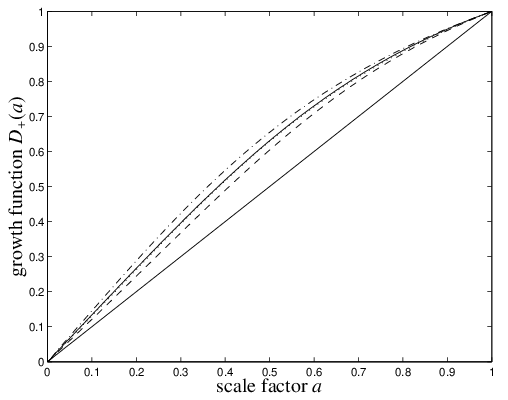
Fig. 2 shows the growth functions $D_{+}(a)$ (normalised to unity today) in the four cosmologies considered. Evolving dark energy has the property of suppressing structure formation at an earlier time, which can be partially compensated by CDM decay (because the gravitational fields generated by the overdensity $\delta(\mn@boldsymbol{x})$ are stronger if $\Omega_{m}(a)$ has a higher value), hinting at degeneracies between the equation of state parameters and the CDM decay rate. The $\Lambda$CDM and $\phi_{\Gamma}$CDM-models, for example, are almost indistinguishable. The influence of the two terms $3+\mathrm{d}\ln H/\mathrm{d}\ln a$ and $\Omega_{m}(a)$ on the evolution of the growth factor $D_{+}(a)$ is discussed in Appendix A.

The non-standard scaling of the CDM density with scale factor makes it impossible to carry out a number of simplifications when deriving the weak lensing convergence. Substituting the critical density $\rho_{\mathrm{crit}}(a)=3H^{2}(a)/(8\pi G)$ with $\langle\rho\rangle(a)=\Omega_{m}(a)\rho_{\mathrm{crit}}(a)$ into the expression $\Delta\Phi=4\pi Ga^{2}\>\langle\rho\rangle(a)\>\delta$ for the comoving Poisson equation yields

with explicit functions $H(a)$ and $\Omega_{m}(a)$. Using this expression one obtains for the weak lensing convergence (Bartelmann & Schneider, 2001)

Inclusion of the redshift distribution of background galaxies and reformulating the integration yields:

where we abbreviated

with the redshift distribution $p(z)\mathrm{d}z$ of the lensing galaxies. From that one finds an analogous expression for the convergence spectrum (Limber, 1954),

which results from projection of the CDM spectrum $P(k)$. The standard results are recovered by setting

which is valid only for stable CDM-models. The lensing efficiency function $W(\chi)$ can be isolated from the above expresssions, yielding

Lensing efficiency functions $W(\chi)/\chi$ for the four exemplary cosmologies are given in Fig. 3: At low redshifts, models with evolving dark energy attain higher values for $W(\chi)$ compared to models with a cosmological constant, and at high redshifts, models with decaying CDM have higher values for $W(\chi)$ compared to models with stable CDM, with an interesting crossing at a distance of $\simeq 100~\mathrm{Mpc}/h$. This behaviour is caused by the evolution of $H(a)$ as discussed in the previous section and indicates that it is possible to increase the redshift at which the lensing signal originates by increasing $\Gamma$ and by choosing an equation of state model with mean $w$ close to $-1$.

Fig. 4 illustrates the impact of CDM decay on linear convergence power spectra: Models with decaying CDM exhibit larger values for the power spectrum, which is due to the fact that in these models the matter density in the past was higher compared to models with stable CDM, which leads to stronger gravitational potentials and hence a stronger light deflection, which is described by the higher values of the lensing efficiency function $W(\chi)$, with a minor effect from the growth function $D_{+}(a)$. This feature might in fact be able to reconcile the high value for $\sigma_{8}$ required by weak lensing surveys with the $\sigma_{8}$ value following from CMB data, by generating high values for the lensing signal with a comparatively small value for $\sigma_{8}$, if one allows for CDM-decay.

In summary, the lensing signal measures a combination of structure growth $D_{+}(a)$, coupling strength $\Omega_{m}(a)$ and geometrical factor $\chi(a)$, which all are influenced by the interaction term in the evolution equations for the dark matter and dark energy density and make up the form of the lensing efficiency $W(\chi)$ and the finally the expression for the spectra $C_{\kappa}(\ell)$ and $B_{\kappa}(\ell_{1},\ell_{2},\ell_{3})$. The epoch-varying coupling of the light to the gravitational potential, due to the non-standard Poisson equation eqn. (7) is an important mechanism, which is not clearly treated in La Vacca & Colombo (2008). It is worth noting that models with interacting dark fluids constitute a new class of models in this respect, in comparison to models with non-interacting evolving dark energy.

Concerning the numerical evaluation, we generate a lookup table with 200 values of the relation between scale factor and comoving distance $a(\chi)$, the Hubble function $H(a)$, the growth function $D_{+}(a)$, the matter density parameter $\Omega_{m}(a)$, and finally the nonlinear wave vector $k_{\mathrm{nlin}}$ for a given cosmological model and use cubic splines for interpolating between these values. Additionally, values for the tomography lensing efficiency functions $G_{i}(\chi)$ for each redshift bin $i$ are cached, as a function of comoving distance. These measures provide a significant speed-up in all computations, because we do not have to reevaluate the densities $\rho_{m}$ and $\rho_{\phi}$ for each time step, to solve for the Hubble function $H(a)$ and the density parameter $\Omega_{m}(a)$, and use these results for computing the growth function $D_{+}(a)$, the comoving distance $\chi$ and the lensing efficiency function $G_{i}(\chi)$.

For the linear power spectrum $P(k)$, which describes the fluctuation amplitude of the density field $\delta(\mn@boldsymbol{k})$, $\langle\delta(\mn@boldsymbol{k})\delta(\mn@boldsymbol{k}^{\prime})\rangle=(2\pi)^{3}\delta_{D}(\mn@boldsymbol{k}+\mn@boldsymbol{k}^{\prime})P(k)$, we make the ansatz

The shape of the transfer function $T(k)$ is well approximated by the fitting formula suggested by Bardeen et al. (1986),

where the wave vector $k=q\Gamma_{s}$ is rescaled with the shape parameter $\Gamma_{s}$ (Sugiyama, 1995),

The fluctuation amplitude is normalised to the value $\sigma_{8}$ on the scale $R=8~\mathrm{Mpc}/h$,

with a Fourier-transformed spherical top-hat $W(x)=3j_{1}(x)/x$ as the filter function. $j_{\ell}(x)$ denotes the spherical Bessel function of the first kind of order $\ell$ (Abramowitz & Stegun, 1972).

The first order contribution to the bispectrum $B_{\delta}(\mn@boldsymbol{k}_{1},\mn@boldsymbol{k}_{2},\mn@boldsymbol{k}_{3})$ of the density field from nonlinear structure formation is given by (Fry, 1984a; Fry, 1984b; Takada & Jain, 2003a):

with the classical mode coupling functions,

which is replaced by the mode coupling function in hyper-extended perturbation theory,

where $x=\mn@boldsymbol{k}_{i}\mn@boldsymbol{k}_{j}/\left(k_{i}k_{j}\right)$ denotes the cosine of the angle between $\mn@boldsymbol{k}_{i}$ and $\mn@boldsymbol{k}_{j}$. The coefficients $a(k)$, $b(k)$ and $c(k)$ are given by (Scoccimarro & Frieman, 1999; Scoccimarro & Couchman, 2001):

where the time evolution of the fluctuation amplitude is given by the linear growth function, $\sigma_{8}(z)=D_{+}(z)\sigma_{8}$. The wave vectors are rescaled with the nonlinear wave number, $q\equiv k/k_{\mathrm{NL}}$. The logarithmic slope of the linear power spectrum,

can be straightforwardly determined with the polynomial fit to the transfer function $T(k)$. The nonlinear wave number at scale factor $a$ is given by the scale at which the variance $\sigma$ of the density fluctuations becomes unity,

Finally, the saturation parameter $Q(n)$ can be computed from the logarithmic slope $n$ of the linear CDM spectrum,

Furthermore, we use the parameterisation proposed by Smith et al. (2003) for the nonlinear CDM spectrum $P_{\mathrm{NL}}(k)$ and its slow time evolution, which is particularly useful as the time evolution is parameterised with $\Omega_{m}(a)$.

The spherical bispectrum $B_{\kappa}(\ell_{1},\ell_{2},\ell_{3})$ is related to the flat-sky bispectrum $B_{\kappa}(\mn@boldsymbol{\ell}_{1},\mn@boldsymbol{\ell}_{2},\mn@boldsymbol{\ell}_{3})$ by (Miralda-Escude, 1991; Kaiser, 1992)

where

$x=\cos\theta$, denotes the Wigner-$3j$ symbol, which results from integrating over three Legendre polynomials $P_{\ell}(x)$. The Wigner-$3j$ symbol cancels non-admissible configurations which would violate the triangle inequality $\left|\ell_{i}-\ell_{j}\right|\leq\ell_{k}\leq\ell_{i}+\ell_{j}$ (Abramowitz & Stegun, 1972). We use the Limber-equation (Limber, 1954) in the flat-sky approximation,

with $\mn@boldsymbol{k}_{p}=\mn@boldsymbol{\ell}_{p}/\chi$, $p=1,2,3$, for projection of the angular convergence bispectrum $B_{\kappa}$. The factorials in the Wigner-$3j$ symbol are evaluated using the Stirling-approximation for the $\Gamma$-function, $\Gamma(n+1)=n!$ with

for $x\gg 1$ (Abramowitz & Stegun, 1972). The resulting approximation for the Wigner-$3j$ symbol overestimates the true value on average by $\simeq 0.4$% in the relevant $\ell$-range. Weak lensing convergence bispectra resulting from this procedure are shown in Fig. 5 for the equilateral configuration. As in the case of the convergence spectra $C_{\kappa}(\ell)$, the bispectra $B_{\kappa}(\ell_{p})$ attain higher values in models with decaying CDM compared to those with stable CDM. This increase amounts to $\simeq 10$%, and is observed independent of the equation of state of dark energy, where one observes a change of a few percent in the models with a cosmological constant relative to those with a varying equation of state.

Lensing convergence bispectra for isosceles triangles are given in Fig. 6, for $\ell=10^{3}$. The plot suggests that the increase in power observed in decaying CDM models is present for all configurations, if the background galaxy distribution has a high average redshift, which is in fact expected for a change of cosmology on the homogeneous level. Again, typical differences between models with stable CDM and those with $\Gamma=1/3$ amount to $\simeq 10\%$, irrespective of the opening angle of the triangle.

Fig. 7 illustrates the configuration dependence of the weak lensing bispectra, for $\ell_{3}=1000$. In particular, the plot shows the configuration dependence variable $R_{\ell_{3}}(\ell_{1},\ell_{2})$,

for $\ell_{3}=10^{3}$. Differences in cosmology are cancelled in first order in this expression, and for that reason the plot only shows the bispectrum configuration dependence for the fiducial $\Lambda$CDM model.

In the case of bispectrum tomography, where the background galaxies are divided in to two or more redshift bins $(i,j,k)$, eqn. (28) generalises to

with indidual weighting functions

where the lensing-kernel weighted redshift distribution is given by

The tomography bins are chosen to contain equal numbers of background galaxies, which are distributed in redshift $z$ according to (Smail et al., 1995),

where the distribution is characterised by the parameters $\beta=\frac{3}{2}$ and $z_{0}=0.64$ (corresponding to a median redshift of $z_{\mathrm{med}}=0.9$, c.f. Appendix B). We will consider 2-bin tomography, because any finer subdivision does not necessarily improve the bounds on cosmological parameters due to the high covariance of the signal originating from different tomography bins, as discussed in Takada & Jain (2003b); Takada & Jain (2004).

The observed bispectra $\tilde{B}_{(ijk)}(\ell_{1},\ell_{2},\ell_{3})$ are unbiased estimates of the true bispectra $B_{(ijk)}(\ell_{1},\ell_{2},\ell_{3})$,

because the intrinsic ellipticity distribution $p(\epsilon)\mathrm{d}\epsilon$ of the background galaxies is assumed to be skewless. But $p(\epsilon)\mathrm{d}\epsilon$ has a finite width $\sigma_{\epsilon}$, which impacts on the observed power spectra $\tilde{C}_{ij}(\ell)$ (Kaiser, 1998; Hu, 1999),

$n_{i}$ is the number of galaxies per steradian in the tomography bin $i$,

with the total number of galaxies per steradian $n$. The bispectrum covariance for tomography, which is diagonal in $\ell_{p}$, $p=1,2,3$, is approximated by (Hu, 2000; Takada & Jain, 2003b; Takada & Jain, 2004)

where the function $\Delta(\ell_{p})$ counts the multiplicity of triangle configurations and is defined as

$f_{\mathrm{sky}}$ denotes the fraction of the observed sky. It is worth noting that the bispectra $B_{(ijk)}(\ell_{1},\ell_{2},\ell_{3})$ are invariant under permutations of the bin indices. Because of that, there are 4 independent bispectra for 2-bin tomography, which can be conveniently indexed with the number $q=2^{i}+2^{j}+2^{k}$.

The Fisher matrix $F_{\mu\nu}^{\mathrm{GL}}$ for the parameter space consisting of $x\in\{\Omega_{m},\sigma_{8},w_{0},w_{a},\Gamma,h\}$ is constructed with $\Lambda$CDM as the fiducial cosmological model. Particularly, for measurements of the weak lensing bispectrum $B_{(ijk)}(\ell_{1},\ell_{2},\ell_{3})$, one obtains:

with $\ell_{p}\in\{\ell_{1},\ell_{2},\ell_{3}\}$. The summation is carried out with the condition $\ell_{1}\leq\ell_{2}\leq\ell_{3}$, such that every triangle configuration is counted once, between the limits $\ell_{\mathrm{min}}=10^{2}$ and $\ell_{\mathrm{max}}=2\times 10^{3}$. The indices $i,j,k$ and $l,m,n$ run over the tomography bins.

Following Takada & Jain (2003b); Takada & Jain (2004), we use binned summations in the multipoles $\ell_{1}$ and $\ell_{2}$, but carry out an unbinned summation in $\ell_{3}$ in order to account for the vanishing Wigner-$3j$ symbol if $\sum_{p}\ell_{p}$ is an odd number and for the sign change of the Wigner-$3j$ symbol depending on whether $\sum_{p}\ell_{p}~\mathrm{mod}~4$ vanishes or not. Using $\Delta\ell_{1}=\Delta\ell_{2}=25$, the computational load is reduced by three orders of magnitude, as we have to compute $2\times 10^{7}$ triangles instead of $3\times 10^{10}$ triangles, for $l_{\mathrm{max}}=2\times 10^{3}$. Using binned summation in two variables is well justified, given the smooth variation of the bispectrum illustrated in Fig. 7. The scale on which the numerical derivatives are computed corresponds to a 5% variation for $\Omega_{m}$, $\sigma_{8}$ and $h$ and to a 10% variation for the dark energy parameters $w_{0}$, $w_{a}$ and $\Gamma$.

We would like to emphasise at this point that our Fisher-analysis implicitly assumes priors on (i) spatial flatness, $\Omega_{m}+\Omega_{\phi}=1$, which affects all geometrical measures, (ii) the baryon density $\Omega_{b}$, which adds a correction to the shape parameter, and finally (iii) the slope $n_{s}$ of the CDM spectrum $P(k)$ for small wave numbers $k$. We neglect the influence of $\Omega_{b}$, because the baryons cause only a minor correction to the shape parameter, and keep $n_{s}=1$ and $\Omega_{m}+\Omega_{\phi}=1$ fixed, as they are both generic predictions of inflation and well tested by CMB observations. The parameter space considered here is motivated by the fact that $\Omega_{m}$, $w_{0}$, $w_{a}$ and $\Gamma$ all increase the lensing signal, either by their influence on the growth equation or by appearing in the Poisson equation, and are naturally degenerate with $\sigma_{8}$. As additional priors to the lensing measurement, we assume $1\sigma$-errors from PLANCK CMB observations with the numerical values $\Delta h=0.13$ and $\Delta\sigma_{8}=0.01$ (Eisenstein et al., 1999). The priors are assumed to be diagonal, $F_{\mu\nu}^{\mathrm{CMB}}=\delta_{\mu\nu}/\sigma_{\mu}^{2}$, and added to the lensing Fisher matrix $F_{\mu\nu}^{\mathrm{GL}}$,

because the likelihoods of independent measurements can be multiplied and their $\chi^{2}$-functions added.

The diagonal elements of the inverse Fisher matrix give the Cramér-Rao bound on individual parameters,

which are compiled in Table 3 for 2-bin weak lensing tomography, with the enhancement of the measurement by including CMB-priors on $\sigma_{8}$ and on $h$. Quite generally, weak lensing bispectrum tomography with DUNE in conjunction with CMB priors provides percent errors on $\Omega_{m}$, $\sigma_{8}$ and $h$, errors of the order of 20% on $w_{0}$ and $\Gamma$, but a weak constraint on $w_{a}$, which is due to the fact that in comparing to the analysis by Takada & Jain (2004), the DUNE galaxy sample has a much lower median redshift (0.9 compared to 1.5) and hence a weaker lever arm on $w_{a}$.

The constraint on $\Delta\Gamma\simeq 0.13$ translates to a lower bound on the CDM lifetime of more than 7.7 Hubble times, corresponding to $t_{\Gamma}\lower 2.15277pt\hbox{$\;\mathrel{\mathop{\kern 0.0pt\sim}\limits^{>}}\;$}75.3/h$ Gyr. Limits on the CDM particle lifetime from lensing measurements of that order of magnitude may serve to exclude certain particle candidates, but we should emphasise that we investigate only a single decay channel with an unknown branching ratio $b$: If CDM has two decay modes with the probabilities $b$ for decaying into dark energy and $1-b$ for decaying into other products, with corresponding decay rates $\Gamma_{\phi}$ (constrained by lensing) and $\Gamma_{X}$, the total decay rate is given by $\Gamma=b\Gamma_{\phi}+(1-b)\Gamma_{X}$.

The $\chi^{2}$-value for pairs of parameters $(x_{\mu},x_{\nu})$ can be computed from the inverse $(F^{-1})_{\mu\nu}$ of the Fisher matrix (Matsubara & Szalay, 2002),

where $\Delta x_{\mu}=x_{\mu}-x_{\mu}^{\Lambda\mathrm{CDM}}$. Specifically, the contour at

encloses a fraction of $\mathrm{erf}(n/\sqrt{2})$ of parameter space, which corresponds to a confidence level of $n\sigma$. $\mathrm{erf}(x)$ and $\mathrm{erfc}(x)=1-\mathrm{erf}(x)$ are the error function and the complementary error function, respectively (Abramowitz & Stegun, 1972). The correlation coefficient $r_{\mu\nu}$ is defined as

and describes the degree of dependence between the parameters $x_{\mu}$ and $x_{\nu}$ by assuming numerical values close to 0 for independent, and close to 1 for strongly dependent parameters. Constraints on pairs $(x_{\mu},x_{\nu})$ of cosmological parameters from the Fisher-analysis are compiled in Fig. 8, along with the respective correlation coefficient $r_{\mu\nu}$.

The CDM decay constant $\Gamma$ is negatively correlated with $\Omega_{m}$ because a simultaneous decrease of the matter density today as well as a increase in the decay constant leads to the same averaged matter density for the lensing signal. The degeneracies with $w_{0}$ and $w_{a}$ are such that $w_{0}$ has to be de- and $w_{a}$ increased in order to have the same lensing signal in models with non-vanishing $\Gamma$. The positive correlation of $\Gamma$ with $\sigma_{8}$ is a projection effect in the marginalisation driven by the tight constraints between $\Omega_{m}$, $w_{0}$ and $h$, and the classical degeneracies between $\Omega_{m}$ and $\sigma_{8}$ (the power spectrum normalisation and the strength of the gravitational potentials) and between $\Omega_{m}$ and $h$ (the definition of the shape parameter) are recovered.

We would like to point out that the effective equation of state parameter $w_{\mathrm{eff}}$ may cross the boundary towards phantom models, for which $w<-1$,

with $H(a)=H_{0}h(a)$, if decay is considered. Therefore, we mark the forbidden regions of parameter space in the relevant plots.

Generalising eqn. (43) to three parameters $(x_{\mu},x_{\nu},x_{\rho})$ yields

In a 3-dimentional parameter space, the contours at $\Delta\chi_{1}^{2}\simeq 2.6124$ and $\Delta\chi_{2}^{2}\simeq 4.2222$ correspond to significance levels of $1\sigma$ and $2\sigma$, respectively. Figs. 9 and 10 summarise simultaneous constraints on the triplets $(\sigma_{8},w_{0},\Gamma)$ and $(\Omega_{m},\sigma_{8},\Gamma)$, respectively. The increase in lensing signal by either increasing $\sigma_{8}$ or the dark energy equation of state $w_{0}$ is illustrated in Fig. 9, with the weak degeneracy that models with decaying CDM require higher values of $\sigma_{8}$, for lensing at low redshift. Fig. 10, on the contrary, shows that $\sigma_{8}$ can be decreased in models with decay if $\Omega_{m}$ is increased at the same time.

References

- Abramowitz & Stegun (1972) Abramowitz M., Stegun I. A., 1972, Handbook of Mathematical Functions. Handbook of Mathematical Functions, New York: Dover, 1972
- Bardeen et al. (1986) Bardeen J. M., Bond J. R., Kaiser N., Szalay A. S., 1986, ApJ, 304, 15
- Bartelmann & Schneider (2001) Bartelmann M., Schneider P., 2001, Physics Reports, 340, 291
- Benabed & Bernardeau (2001) Benabed K., Bernardeau F., 2001, Phys. Rev. D, 64, 083501
- Bernardeau et al. (1997) Bernardeau F., van Waerbeke L., Mellier Y., 1997, A&A, 322, 1
- Bernstein & Jain (2004) Bernstein G., Jain B., 2004, ApJ, 600, 17
- Boehmer et al. (2008) Boehmer C. G., Caldera-Cabral G., Lazkoz R., Maartens R., 2008, ArXiv 0801.1565, 801
- Boughn & Crittenden (2003) Boughn S. P., Crittenden R. G., 2003, in Holt S. H., Reynolds C. S., eds, The Emergence of Cosmic Structure Vol. 666 of American Institute of Physics Conference Series, The Absence of the Integrated Sachs-Wolfe Effect: Constraints on a Cosmological Constant. pp 67–70
- Chevallier & Polarski (2001) Chevallier M., Polarski D., 2001, International Journal of Modern Physics D, 10, 213
- Dodelson & Zhang (2005) Dodelson S., Zhang P., 2005, Phys. Rev. D, 72, 083001
- Eisenstein et al. (1999) Eisenstein D. J., Hu W., Tegmark M., 1999, ApJ, 518, 2
- Fry (1984a) Fry J. N., 1984a, ApJL, 277, L5
- Fry (1984b) Fry J. N., 1984b, ApJ, 279, 499
- Giannantonio et al. (2006) Giannantonio T., Crittenden R. G., Nichol R. C., Scranton R., Richards G. T., Myers A. D., Brunner R. J., Gray A. G., Connolly A. J., Schneider D. P., 2006, Phys. Rev. D, 74, 063520
- Giannantonio et al. (2008) Giannantonio T., Scranton R., Crittenden R. G., Nichol R. C., Boughn S. P., Myers A. D., Richards G. T., 2008, ArXiv 0801.4380, 801
- Heavens (2003) Heavens A., 2003, MNRAS, 343, 1327
- Hu (1999) Hu W., 1999, ApJL, 522, L21
- Hu (2000) Hu W., 2000, Phys. Rev. D, 62, 043007
- Hu (2002) Hu W., 2002, Phys. Rev. D, 66, 083515
- Jain & Seljak (1997) Jain B., Seljak U., 1997, ApJ, 484, 560
- Jain & Taylor (2003) Jain B., Taylor A., 2003, Physical Review Letters, 91, 141302
- Kaiser (1992) Kaiser N., 1992, ApJ, 388, 272
- Kaiser (1998) Kaiser N., 1998, ApJ, 498, 26
- Kilbinger & Schneider (2005) Kilbinger M., Schneider P., 2005, A&A, 442, 69
- La Vacca & Colombo (2008) La Vacca G., Colombo L. P. L., 2008, ArXiv e-prints, 803
- Limber (1954) Limber D. N., 1954, ApJ, 119, 655
- Linder & Jenkins (2003) Linder E. V., Jenkins A., 2003, MNRAS, 346, 573
- Matsubara & Szalay (2002) Matsubara T., Szalay A. S., 2002, ApJ, 574, 1
- Mellier (1999) Mellier Y., 1999, ARA&A, 37, 127
- Miralda-Escude (1991) Miralda-Escude J., 1991, ApJ, 380, 1
- Nolta et al. (2003) Nolta M. R., Devlin M. J., Dorwart W. B., Miller A. D., Page L. A., Puchalla J., Torbet E., Tran H. T., 2003, ApJ, 598, 97
- Olivares et al. (2006) Olivares G., Atrio-Barandela F., Pavón D., 2006, Phys. Rev. D, 74, 043521
- Rassat et al. (2007) Rassat A., Land K., Lahav O., Abdalla F. B., 2007, MNRAS, 377, 1085
- Refregier (2003) Refregier A., 2003, ARA&A, 41, 645
- Schneider & Bartelmann (1997) Schneider P., Bartelmann M., 1997, MNRAS, 286, 696
- Schneider et al. (1992) Schneider P., Ehlers J., Falco E. E., 1992, Gravitational Lenses. Springer-Verlag Berlin Heidelberg New York.
- Scoccimarro & Couchman (2001) Scoccimarro R., Couchman H. M. P., 2001, MNRAS, 325, 1312
- Scoccimarro & Frieman (1999) Scoccimarro R., Frieman J. A., 1999, ApJ, 520, 35
- Smail et al. (1995) Smail I., Hogg D. W., Blandford R., Cohen J. G., Edge A. C., Djorgovski S. G., 1995, MNRAS, 277, 1
- Smith et al. (2003) Smith R. E., Peacock J. A., Jenkins A., White S. D. M., Frenk C. S., Pearce F. R., Thomas P. A., Efstathiou G., Couchman H. M. P., 2003, MNRAS, 341, 1311
- Spergel et al. (2003) Spergel D. N., Verde L., Peiris H. V., Komatsu E., Nolta M. R., Bennett C. L., Halpern M., Hinshaw G., Jarosik N., Kogut A., Limon M., Meyer S. S., Page L., Tucker G. S., Weiland J. L., Wollack E., Wright E. L., 2003, ApJS, 148, 175
- Sugiyama (1995) Sugiyama N., 1995, ApJS, 100, 281
- Takada & Jain (2003a) Takada M., Jain B., 2003a, MNRAS, 340, 580
- Takada & Jain (2003b) Takada M., Jain B., 2003b, MNRAS, 344, 857
- Takada & Jain (2004) Takada M., Jain B., 2004, MNRAS, 348, 897
- Tegmark et al. (1997) Tegmark M., Taylor A. N., Heavens A. F., 1997, ApJ, 480, 22
- Turner & White (1997) Turner M. S., White M., 1997, Phys. Rev. D, 56, 4439
- Valiviita (2008) Valiviita J., 2008, Phys. Rev. D. in preparation
- Wang & Steinhardt (1998) Wang L., Steinhardt P. J., 1998, ApJ, 508, 483
Appendix A Growth function
The growth function is a solution to the differential equation