Simulations of Sisyphus cooling including multiple excited states

Laser cooling is a generic name for a number of techniques that use laser light to cool atoms down to millikelvin or even microkelvin temperatures [1]. Today, laser cooling is used in numerous applications, for instance as one of the steps used in the process to create a Bose-Einstein condensate [2], in atomic clocks [3], and other high-precision experiments using atoms.

The most commonly used technique, Doppler cooling, has as its lower limit the Doppler temperature, which for most atoms is of the order 0.1 mK [1]. However, lower temperatures can be reached in near-resonant optical lattices, i.e., standing waves of laser light with periodical, spatially alternating polarisations [4, 5]. In these systems temperatures approaching the recoil limit of a few $\mu$K can be achieved [6]. This result first came as a surprise, but was soon given a theoretical model in form of the so-called Sisyphus mechanism [7, 8]. In this model a combination of spatially dependent optical pumping rates between the magnetic sublevels of the atom, together with the periodic potentials of the optical lattice, give rise to an effective friction which causes cooling of the atoms.

Whereas the Sisyphus model successfully describes many of the qualitative features of laser cooling in optical lattices, it is not sufficient for a quantitative analysis. For this purpose a number of numerical techniques have been developed, e.g., semiclassical methods based on Fokker-Planck-like equations [9, 10], a band-structure model [11], and quantum Monte Carlo simulations [12]. (For a review see reference [5].) These theoretical techniques have gone a long way in reproducing experimental findings. However, unexplained features still remain. For instance, theoretical simulations have consistently given kinetic temperatures of the atoms which are independent of the laser detuning from the atomic resonance, except very close to this resonance [13]. Experimental results show that this is largely true for large potential depths (large laser irradiances), where the kinetic temperature is a linear function of the potential depth. However, as the laser irradiance is lowered a minimum temperature is achieved, before the temperature starts to rapidly increase for even lower irradiances. The point of this minimum is often referred to as décrochage. Experiments have shown that, in contrast to theoretical predictions, the point of décrochage does depend on detuning [14, 15, 16].

Hitherto all theoretical simulations have used a simplified level structure of the atom. It has been assumed that the cooling process only depends on optical pumping via a single excited state. However, the excited state is really a manifold of several closely-lying hyperfine states. In caesium the excited state used has total angular momentum $F_{\mathrm{e}}=5$. However, separation between the $F_{\mathrm{e}}=5$ and $F_{\mathrm{e}}=4$ excited states is only $48.1\Gamma$ ($\Gamma$ being the natural linewidth), which is comparable to typical detunings in experiments. A recent experiment showed that even for detunings very close to the $F_{\mathrm{e}}=4$ state, the proximity to this state did not seem to have any effect on the temperature [15]. This seems to underpin the assumption that this state can be neglected in simulations. Nevertheless, it is still possible that the $F_{\mathrm{e}}=4$ state is important for the cooling process close to décrochage. In this paper this possibility is investigated using semiclassical simulations including both the $F_{\mathrm{e}}=5$ and $F_{\mathrm{e}}=4$ states of the hyperfine manifold.

In an earlier publication we developed a novel semiclassical method for Sisyphus cooling [10], and showed that this method gives excellent agreement with the fully quantum-mechanical method [12]. In the semiclassical method the external degrees of freedom, i.e., position and momentum, are treated as simultaneously well-defined classical variables. The internal degree of freedom, i.e., the magnetic substate, is on the other hand treated fully quantum mechanically, allowing for arbitrary superpositions. In this way we are able to generalize the simplified $F_{\mathrm{g}}=1/2\rightarrow F_{\mathrm{e}}=3/2$ model to realistic angular momenta, $F_{\mathrm{g}}=4\rightarrow F_{\mathrm{e}}=5$ for Cs, while retaining an excellent agreement with fully quantum-mechanical simulations. This is in contrast to, e.g., the treatment in reference [9] where the internal states were projected onto an adiabatic basis. Our method automatically includes all couplings between adiabatic (or diabatic) states, which were neglected in reference [9]. Inclusion of these couplings has been showed to be crucial for good agreement with fully quantum-mechanical simulations [10].

Having established the validity of our method, we now continue onto more detailed investigations of the cooling process. We first extend our method to include two excited hyperfine states. The generalized optical Bloch equations for an atom of mass $m$ with a ground state ${\mathrm{g}}$ and two excited states ${\mathrm{e}}1$ and ${\mathrm{e}}2$ are

Here $\sigma$ is the density matrix of the atom, including the ground state ${\mathrm{g}}$ and both excited states ${\mathrm{e}1}$ and ${\mathrm{e}2}$,

where each $\sigma_{ij}$ is a submatrix with rows and columns corresponding to the different magnetic sublevels. The Hamiltonian part of the evolution is determined by the kinetic term, the atomic internal Hamiltonian ${\mathrm{H}}_{\mathrm{A}}$ and the atom-laser interaction $V_{\mathrm{AL}}$. Setting the zero of energy at the ground state, the atomic Hamiltonian is just

with $\hbar\omega_{F_{\mathrm{e}}}$ the energy of the excited states. The atom-laser interaction takes the form

where $G_{\mathrm{e}}$ represents the simultaneous absorption of a photon and excitation of the atom in the excited level $\mathrm{e}$, while $G_{\mathrm{e}}^{\dagger}$ represents the inverse emission process. The matrix elements $G_{\mathrm{e}}$ are products of the appropriate transition dipoles ${\bf d}$ and the positive frequency component ${\bf E}^{+}$ of the laser field

with ${\boldsymbol{\xi}}$ the (position-dependent) polarisation vector. In the basis of the magnetic substates, $M_{\mathrm{e}}=-F_{\mathrm{e}},-F_{\mathrm{e}}+1,\dots,F_{\mathrm{e}}$ (${\mathrm{e}}={\mathrm{e}1}$ or ${\mathrm{e}2}$), the transition dipole is the product of a reduced matrix element and a Clebsch-Gordan coefficient,

and ${\boldsymbol{\epsilon}}_{q}$ are the usual spherical polarisation vectors. The polarisation vector ${\boldsymbol{\xi}}$ is chosen as the one-dimensional lin$\perp$lin laser configuration [5],

with $k$ the wave vector of the laser. The final term in equation (1) describes the transfer of populations and damping of coherences due to spontaneous emission

where $\Gamma_{\mathrm{e}}$ is the partial width of the excited state ${\mathrm{e}}$ for decay to the ground state ${\mathrm{g}}$. (Where decay to hyperfine states other than ${\mathrm{g}}$ are possible, most experimental set-ups include a repumper laser which brings the atom back to the excited state.) Here $\gamma_{\mathrm{gg}}$ includes both the recoil and the probabilities of populating different ground states after a cycle of optical pumping through either of the two excited states,

In most cases of interest, the irradiance of the lasers is sufficiently low that the population of the excited states is much smaller than the ground-state population, i.e., the transitions are far from saturation. This condition can be expressed in terms of the saturation parameters $s_{\mathrm{e}1}$ and $s_{\mathrm{e}2}$ as

where $\Omega_{\mathrm{e}}=-\langle F_{\mathrm{e}}||d||F_{\mathrm{g}}\rangle E_{0}/\hbar$ is the Rabi frequency of the transition and $\Delta_{\mathrm{e}}$ the detuning from the excited state. In the low saturation limit the excited states will rapidly adjust to any change in the ground state density matrix. For time scales relevant to the evolution of the ground state, the excited state density matrices can be expressed as functions of $\sigma_{\mathrm{gg}}$. Through the process of adiabatic elimination of the excited states we then arrive at an effective equation for $\sigma_{\mathrm{gg}}$ only,

where

Here the effective Hamiltonian describing the conservative part of the evolution is given by

The matrix

describes the coherent couplings and light shifts of the magnetic substates. We have also used the conventional notation

In our simulations a semiclassical approximation to equation (14) is used. This approximation is derived by first rewriting equation (14) in terms of the Wigner distribution, which is then Taylor-expanded to second order in $p$. For more details see [10]. This results in a set of coupled Fokker-Planck-like equations for the populations of and coherences between the magnetic substates. Hence, while position and momentum are treated as classical variables, the internal states of the atom are treated fully quantum mechanically. Finally, the evolution equations are converted into a Langevin form. That is, each atom is assigned a time-dependent position $z(t)$ and momentum $p(t)$ (see, e.g., [18]), which follow the classical equations

Here, $f(t)$ is a conservative force and $\eta(t)$ is a diffusive force with the properties

where $\langle\cdot\rangle$ stands for a time average and $D$ is a diffusion coefficient. The forces are calculated as a trace over the magnetic sublevels, where the internal state of an atom is represented by a density matrix $w(t)$. The force is given by

The first term above is the force arising from the second-order light-shift potential, while the second term is the radiation pressure. The diffusion coefficient is given by

with $k_{\mathrm{R}}$ the wave vector of the emitted photon (we neglect the difference in energy of the photons emitted from the two excited states). The first term arises from the recoil from photons spontaneously emitted in random directions, while the second term is connected to fluctuations in the radiation pressure. The evolution equation for the internal-state density matrix is

Finally, we consider the specific case of the $F_{\mathrm{g}}=4$ and $F_{\mathrm{e}1}=4$, $F_{\mathrm{e}2}=5$ states of caesium. Using that $\langle 4||d||4\rangle=\sqrt{7/12}\langle 5||d||4\rangle$ [19] we find that $\Omega_{4}=(7/12)\,\Omega_{5}$. We also have $\Gamma_{5}=\Gamma$, where $\Gamma$ is the natural linewidth, while for the the excited state $F_{\mathrm{e}}=4$ the partial width for decay to the $F_{g}=4$ ground state is $(7/12)\,\Gamma$. The energy separation between the excited states gives $\Delta_{4}=48.1\Gamma+\Delta_{5}$. From these relations the respective saturation parameters (13) and $\Gamma_{\mathrm{e}}^{\prime}$, $\Delta_{\mathrm{e}}^{\prime}$, equations (18), can be derived.

We have performed simulations using 5000 atoms for detunings $\Delta_{5}=-10\Gamma$, $-20\Gamma$, $-30\Gamma$, $-40\Gamma$ and a range of different potential depths (directly proportional to the parameter $\Delta_{5}^{\prime}$). In all simulations the initial temperature was $10\ \mu$K and the time step was ${\rm d}t=0.001/\Gamma^{\prime}_{5}$. The simulations were iterated until the second moment of the momentum distribution had stabilized. It should, however, be noted that since simulations are necessarily performed using a finite number of atoms the moments of the momentum distribution will still fluctuate over time irrespectively of the number of iterations. The typical size of these fluctuations were $\Delta\langle p^{2}\rangle\lesssim p_{\rm R}^{2}$ (where $p_{\rm R}$ is the recoil momentum), but grow for potential depths below décrochage. Depending on detuning and potential depth the number of iterations required for convergence varied between 100000 and 600000. The stability of the results were checked with larger numbers of iterations and with shorter step sizes. It was found that the step size $0.01/\Gamma^{\prime}_{5}$, which was used in reference [10], while working well at $\Delta_{5}=-10\Gamma$ was too coarse for larger detunings.

Our main results are displayed in figure 1, where the one-dimensional temperature $T$, defined as $k_{\mathrm{B}}T/2=\langle p^{2}\rangle/2m$, where $k_{\mathrm{B}}$ is the Boltzmann constant and $m$ the atomic mass, is plotted against $\Delta_{5}^{\prime}$ for different detunings. The value of $\Delta_{5}^{\prime}$ is expressed in terms of the recoil energy gained by the atom after spontaneous emission, $E_{\mathrm{R}}=\hbar^{2}k_{\rm R}^{2}/2m$. We note that for all detunings except $\Delta_{5}=-40\Gamma$, the results for $|\Delta^{\prime}_{5}|\gtrsim 125E_{\mathrm{R}}$ fall on a single line. We thus confirm the experimental finding in reference [15] that the depth of the potential generated by the $4\rightarrow 5$ transition alone provides the appropriate scaling for large potential depths. The results for $\Delta_{5}=-40\Gamma$ have a slightly different slope. Since for this detuning the experimental data in reference [15] only extends up to $\Delta_{5}^{\prime}\simeq 130E_{\mathrm{R}}$ it is not possible to say whether this different slope is an experimental reality.

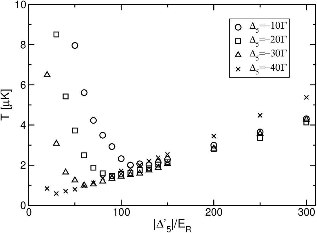
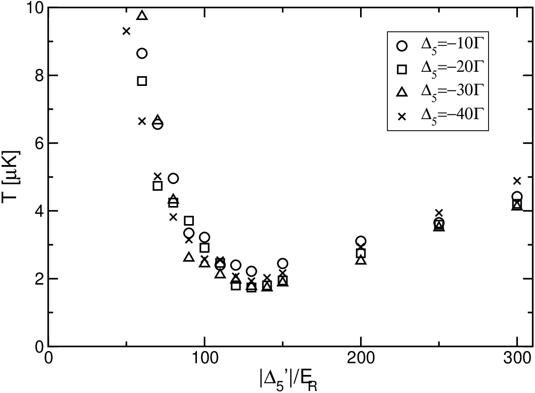
In figure 2 we compare to results of simulations including only the single excited state $F_{\mathrm{e}}=5$. The most striking difference is that in figure 2 the results are essentially independent of detuning over the whole range of potential depths considered. When the additional excited state is included there is a very clear dependence on detuning for shallow potentials, with the linear dependence extending further for larger detunings, giving rise to lower minimum temperatures. For larger detunings the linear behaviour is preserved to a lower potential depth, which makes it possible to reach a lower temperature. This phenomenon has been observed experimentally [14, 15, 16], and has up to now been at variance with all theoretical simulations, semiclassical or fully quantum mechanical. Thus, we can conclude that it is the additional excited state that causes this dependence of the point of décrochage on detuning.

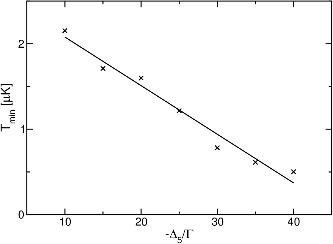
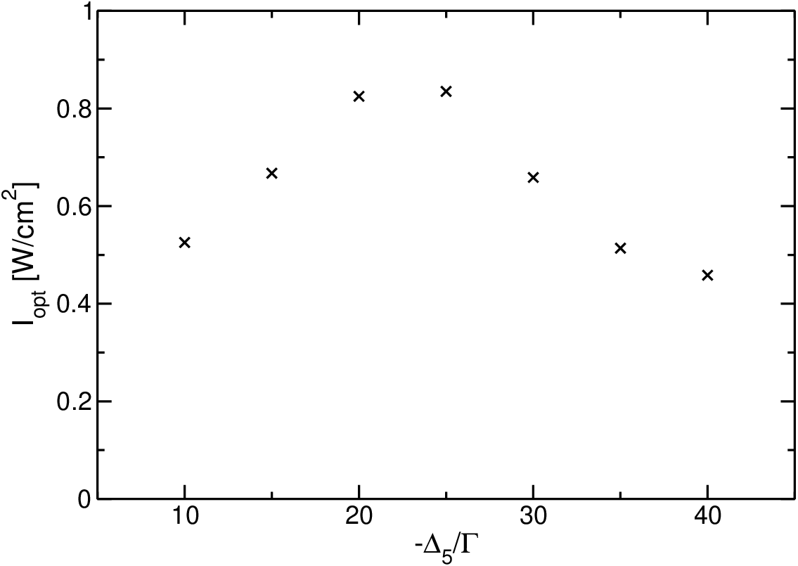
In figure 3 we show the minimum temperature $T_{\rm min}$ achieved at different detunings, while figure 4 gives the laser irradiance at which this minimum was obtained for the same detunings. Around the minimum the simulations give a considerable amount statistical noise. This is particularly true below décrochage, where a very small number of atoms with very high momenta have a significant impact on the value of $\langle p^{2}\rangle$. In order to find the minimum we therefore made simulations for $\Delta_{5}^{\prime}$ in steps of $2E_{\rm R}$ around the minimum, and fitted the results to the functional form $a|\Delta_{5}^{\prime}|+b\exp(-c|\Delta_{5}^{\prime}|)$, with $a$, $b$ and $c$ fit parameters. It was found that this function provides a good fit to simulated data to within the statistical uncertainties. We find that both $T_{\rm min}$ and the optimal potential depth follow a linear dependence on detuning. For $T_{\rm min}$ this is consistent with the results in [14] over the range of detunings considered. In [14, 16] it was also found that the minimum temperature is achieved for an optimal laser irradiance ${\cal I}_{\rm opt}$ independent of detuning. Our results for ${\cal I}_{\rm opt}$ are displayed in figure 4. The optimum irradiance varies almost a factor 2 over the range of detunings investigated, and thus clearly deviates from the experimental result.

At potential depths well above décrochage, the $F_{\mathrm{e}}=4$ level has very little influence. In reference [15] it was reasoned that for trapped atoms the dynamics is mainly determined by the lowest adiabatic potential, as most atoms get optically pumped into the extreme $M_{\mathrm{F}}$ sublevels. This potential is not affected by the $F_{\mathrm{g}}=4\rightarrow F_{\mathrm{e}}=4$ transition. If only the $F_{\mathrm{g}}=4\rightarrow F_{\mathrm{e}}=4$ transition is considered the lowest adiabatic state has vanishing energy at all positions (for detunings to the blue of the line), and is thus dark to the laser light. This readily explains why, as long as the atoms are trapped in the lowest adiabatic potential, their dynamics is determined only by the parameters of the $F_{\mathrm{g}}=4\rightarrow F_{\mathrm{e}}=5$ transition. Even for large detunings the well known scaling of temperature proportional to $I/\Delta_{5}\propto\Delta_{5}^{\prime}$ holds.

Recently the dynamics of laser cooling in optical lattices was interpreted in terms of a bimodal momentum distribution [13, 20, 21, 22]. The atoms are either in an untrapped hot mode or in a cold mode where the atoms are trapped around a potential minimum. As atoms are transferred from the hot to the cold mode the average kinetic temperature decreases. When the system is in steady state the interchange of atoms between the two modes is in balance. For large potential depths essentially all atoms are trapped, giving rise to a truncated Gaussian momentum profile. At lower potential depths the hot mode can be observed even in steady state, giving rise to a deviation from a Gaussian velocity profile in the wings of the distribution.

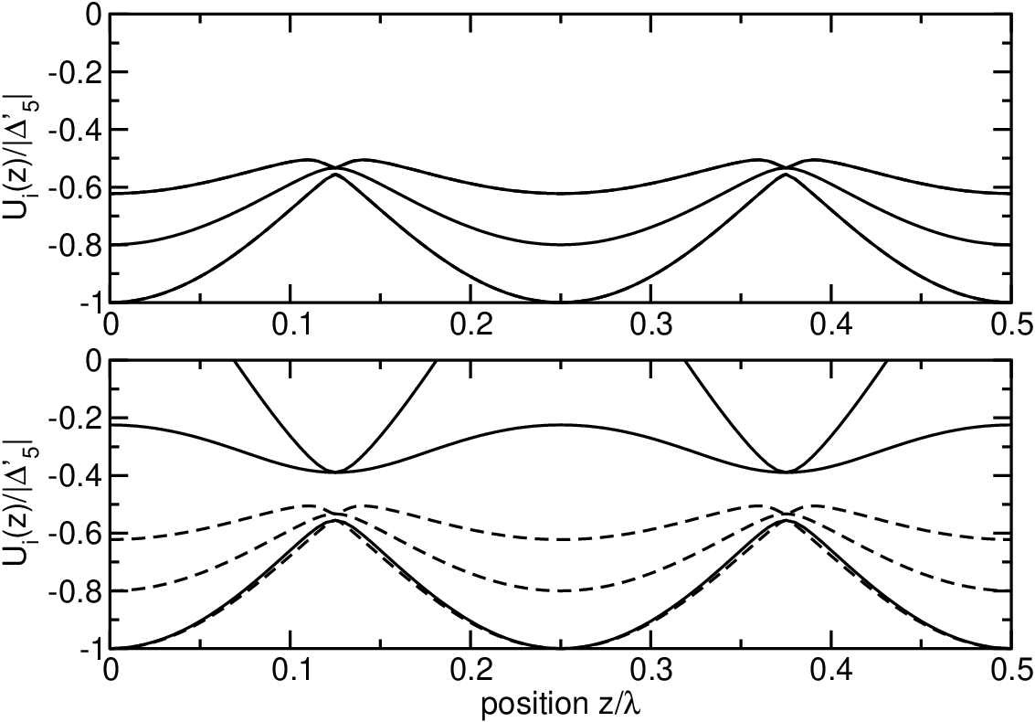
The dependence of the point of décrochage on detuning found in this paper and in reference [15] can also be understood from the bimodal picture of Sisyphus cooling. The cold mode is, as explained above, completely determined by the $F_{\mathrm{g}}=4\rightarrow F_{\mathrm{e}}=5$ transition, and hence its temperature scales proportionally to $\Delta_{5}^{\prime}$ only. According to the bimodal model the hot mode starts to get populated around décrochage, thus driving up the value of $\langle p^{2}\rangle$, even though most atoms are still trapped in the cold mode [21, 22]. Even a relatively small population of the hot mode will dominate the value of $\langle p^{2}\rangle$ since the atoms in this mode have no upper limit for their momenta, and for shallow potentials $\langle p^{2}\rangle$ may even diverge [23]. The increased population of the hot mode is associated with atoms leaving the lowest adiabatic state. Our interpretation of the results in figure 1 is that while the form of the cold mode is unaffected when the $F_{\mathrm{g}}=4\rightarrow F_{\mathrm{e}}=4$ is taken into account, the rate of transfer of atoms from the cold to the hot mode, i.e. away from the lowest adiabatic state, is reduced. As the magnitude of this effect depends on the laser detuning from the $F_{\mathrm{g}}=4\rightarrow F_{\mathrm{e}}=4$ transition a dependence of the point of décrochage on detuning is introduced in this way.

In figure 5  we show the three lowest adiabatic potentials for detunings $\Delta_{5}=-10\Gamma$ and $\Delta_{5}=-40\Gamma$. As noted above the lowest potential is identical for both detunings, giving the same dynamics for both cases. However, as the potential depth is reduced the excited states in figure 5 gain significant populations. Since the potentials of these excited states are very different at different detunings the universal temperature dependence is violated. The universal dependence persists to lower potential depths at large detunings. We therefore conclude that the transfer of atoms to adiabatic states with higher energies is more likely at small detunings, while for large detunings the potential depth has to be lowered even further before this transfer becomes important. As shown in figure 5 at $\Delta_{5}=-10\Gamma$ (and for potentials where the $F_{\rm g}=4\rightarrow F_{\rm e}=4$ transition has been excluded) there are avoided crossings involving the lowest adiabatic potential at $z=\lambda/8$ and $z=3\lambda/8$ ($\lambda$ is the laser wavelength), while for $\Delta_{5}=-40\Gamma$ there are distinct gaps. A tentative conclusion is therefore that the formation of this gap inhibits transfer from the cold to the hot mode, although the details of this effect remains to be worked out.

This interpretation is also supported by the simulated momentum profiles. As an example momentum profiles at $|\Delta_{5}^{\prime}|=20E_{\mathrm{R}}$ at detunings $\Delta_{5}=-10\Gamma$ and $\Delta_{5}=-40\Gamma$ are displayed in figure 6, together with fits to double and single Gaussians respectively. (Fitting also the $\Delta_{5}=-40\Gamma$ profile to a double Gaussian gives no improvement as the widths of the two Gaussians in this case adjust to the same value, indicating that the distribution really is well described by a single Gaussian.) For the smaller detuning the wider hot mode is clearly visible. The fit gives for the cold mode (i.e., the central peak) widths corresponding to $\langle p^{2}\rangle=1.9p_{\mathrm{R}}^{2}$ for $\Delta_{5}=-40\Gamma$ and $\langle p^{2}\rangle=1.4p_{\mathrm{R}}^{2}$ for $\Delta_{5}=-10\Gamma$. Adding the hot mode gives a total $\langle p^{2}\rangle=142p_{\mathrm{R}}^{2}$ for $\Delta_{5}=-10\Gamma$, even though the integral of the Gaussian reveal that both modes contain roughly the same number of atoms (49% hot, 51% cold). Even at the larger detuning a very small number of hot atoms increases $\langle p^{2}\rangle$ to $4.1\,p_{\mathrm{R}}^{2}$. Considering the more than one order of magnitude difference in the overall $\langle p^{2}\rangle$ between the two detunings, we find that the width of the cold mode is remarkably similar, showing that indeed even well below décrochage there is a significant population of the cold mode, with characteristics largely independent of the detuning.

In summary, we showed that at low potential depths, around the so-called point of décrochage, the temperature achieved by Sisyphus cooling does depend on both the potential depth and the detuning from resonance. For these potential depths it is necessary to include several excited hyperfine state in the theoretical description, in order to get accurate results. Simulations including only a single excited hyperfine state show no dependence of the temperature on detuning. This finding agrees very well with the experimental results of references [14, 15, 16], previously unreproduced by simulations. At larger potential depths, where the temperature depends linearly on potential depth, we find that the additional excited hyperfine state has no effect. This is also in agreement with the experimental results in reference [15] that the temperature scales with the potential determined including only the $F_{\rm g}=4\rightarrow F_{\rm e}=5$ transition.