Typical kernel size and number of sparse random matrices over $GF(q)$ - a statistical physics approach

Random matrices over $GF(q)$ are highly important in a number of application areas ranging from biology to computer science and telecommunication. One of the areas where they play a particularly important role is coding theory [1]. In particular, linear codes are defined by the kernel of a parity-check matrix, where each kernel vector is termed a codeword and is associated with an original uncoded message vector by a linear operation defined by a generator matrix. Well known examples include the Hadamard codes, where properties of the kernel and rank play an important role [2], and low-density parity-check codes (LDPC) which provide the best performance to date in many noise regimes. Although the most studied and applied case of LDPC codes is of binary codes over $GF(2)$ there is a significant body of work, of both practical and theoretical nature [3], on codes over more general finite fields showing an improvement in performance with respect to the binary version. In particular, statistical physics based analysis of LDPC codes over $GF(q)$ has been reported in [4].

Low-density parity-check codes are based on random sparse matrices, where the fraction of non-zero elements goes to zero as the size of the matrix increases. In most studies of LDPC codes, it is assumed that a parity-check matrix with $M$ rows (parity-checks) and $N$ columns defines a code of rate $R=1-M/N$, exactly, which is equivalent to the assertion that the number of vectors in the kernel (and therefore the number of codewords) is exactly $q^{NR}$.

In addition to being an interesting applied problem, the properties of these matrices are also of great interest from the pure mathematical point of view and a number of papers has already tried to answer related questions in different instances with a mathematical rigorous approach [5, 6, 7].

In this contribution, we address two key properties of sparse random matrices over $GF(q)$, namely the average dimension of their kernel and the number of matrices for a given connectivity profile, in the case of large matrices. When the matrices are large, keeping $N\rightarrow\infty$ with $M/N$ constant, the problem can be mapped into a system of interacting “spins” and the powerful machinery developed for the study of disordered spin lattices in condensed matter physics can then be used, under some assumptions, to obtain the required properties.

In order to keep this paper as self-contained as possible and make it accessible to a broad readership, we provide in section II a brief introduction to $GF(q)$ matrices and their properties, and to the basic statistical physics methodology on which we have based our analysis. The usual statistical physics approach to the analysis of LDPC codes over the binary field $GF(2)$ is generalized in such a way that it can be efficiently applied to any $GF(q)$ for a general connectivity distribution of non-zero elements and then used to calculate the average kernel dimension of sparse random matrices (SRM) in section IV. Making use of techniques developed in section IV, the number of matrices for a given distribution of non-zero elements is then obtained for various connectivity profiles, in section V. Finally, we present a discussion of the obtained results in section VI.

The transformation

where $\sigma\in{\left\{+1,-1\right\}}$ and $v\in{\left\{0,1\right\}}$, is usually employed to map the $GF(2)$ variables onto the binary representation. This mapping can be generalized to any $GF(q)$ without an intermediate use of the binary field.

Under the operation $\oplus$, $GF(q)$ is homeomorphic to the cyclic group of order $q$ and therefore has a representation as the complex $q$-th roots of unity with the group homeomorphism $\sigma:GF(q)\rightarrow\mathbb{C}$ given by

such that for every $v_{1},v_{2}\in GF(q)$

This mapping has a clear geometric interpretation: $2\pi v/q$ is an angle in the unit circle, such that each element of the Galois field is being mapped onto a spin variable “pointing” in one of $q$ possible angles. Using this mapping allows one to write the null-space constraint for a general vector ${\mathbf{v}}={\left(v^{1},...,v^{N}\right)}\in GF(q)^{N}$ as

with

and

Using the properties of the complex roots of unity, the above quantity $\Delta(q)$ can be shown (see appendix A) to be real and equal to the order $q$ of the field.

Based on this representation, we can now define the “magnetization” of the original system in analogy with the spin system as

and the overlap between two configurations $\sigma$ and $\mbox{\boldmath{$\sigma$}}^{\prime}$ as

where we are now working with the spin variables already mapped to the the complex field $\mathbb{C}$ and therefore the operations of multiplication and addition correspond to the usual ones in $\mathbb{C}$.

It turns out that this kind of representation allows a factorization of the terms simplifying the equations and making the replica calculations simpler, as we will see in the following.

The dimension of the kernel of an $M\times N$ matrix $A$ over $GF(q)$ can be written as $d(A)=\log_{q}\Omega$ where

is the number of vectors in the kernel, $\delta$ is the Kroenecker delta and ${\mathbf{v}}\in GF(q)^{N}$. Direct calculation of $\Omega$ from equation (11) by straightforwardly substituting the Kroenecker delta by its integral representation trivially reproduces the rank-nullity theorem. This calculation is not presented here.

The quantity we are interested in here is the average kernel dimension, more specifically, its density in the limit of large matrices, defined as $Ts$ where

where $1/T=\ln q$ and $M/N\equiv\lambda$, with $\lambda$ a finite positive constant. Using the replica identity (2), we can write

The randomly chosen sparse matrices $A$ have exactly $K_{i}$ non-zero elements in the $i$-th row with probability $\mathcal{P}{\left({\mathbf{K}}\right)}$, ${\mathbf{K}}\equiv{\left(K_{1},...,K_{M}\right)}$, and $C_{j}$ elements in the $j$-th column with probability $\mathcal{P}{\left({\mathbf{C}}\right)}$, ${\mathbf{C}}\equiv{\left(C_{1},...,C_{N}\right)}$, obeying the constraint $\Lambda\equiv\sum_{i}K_{i}=\sum_{j}C_{j}$, where $\Lambda$ is the total number of non-zero elements of the matrix. The elements of $A$ are sampled from the finite field $GF(q)$ with independent equal probabilities $\mathcal{P}{\left(A_{ij}\right)}$.

Let us define, for brevity of notation, $\mathcal{Z}_{n}\equiv{\left<\Omega^{n}\right>_{A}}$. Although the calculations, presented in appendix B, are similar to related calculations in [14, 15], we will use a different approach which is conceptually clearer and has the advantage of allowing later generalizations. In this approach, we sum directly over all entries of the matrix instead of defining a connectivity tensor as used elsewhere [14, 15],

where the average is over the probability distribution $\mathcal{P}{\left({\mathbf{K}},{\mathbf{C}},\Lambda\right)}$ with $\chi{\left(A_{ij}\right)}=0$ if $A_{ij}=0$ and 1 otherwise, and the normalization $\mathcal{N}$ gives the number of matrices which obey the constraints averaged over the distributions of the entries. In this way, any type of constraint on the matrix can be readily included in the calculation, which could be rather cumbersome in other approaches, based on the introduction of a connectivity tensor as the corresponding constraints have to be written in terms of the tensor elements, which can be extremely complicated.

We refer the reader to appendix B for details of the calculations. Using the replica symmetric ansatz, which is shown to be exact for this problem (see appendix D) we arrive at the following self-consistent saddle point equations

with

and to the corresponding expression for $s$

It must be noted that the above equations are only meaningful if $\Lambda\propto N$. A striking property of the above equations is that they are completely independent of the specific distribution of the individual elements of the matrix, depending only on the distribution of ${\mathbf{K}}$ and ${\mathbf{C}}$ (and, obviously, of $\Lambda$).

There exists two straightforward analytical solutions of the above equations, namely, the paramagnetic one given by

and the ferromagnetic solution

When substituted in the above equations, the paramagnetic solution gives the average kernel density as $Ts=1-\lambda=1-M/N$ independently of the order $q$ of the finite field used. In the case of LDPC codes defined by such matrices, this corresponds to random parity-check matrices that defines a code of rate $R=1-\lambda$. The average rank density in this case is $\lambda$. The ferromagnetic solution gives $Ts=0$ and the matrix is full rank; which incidentally means that such matrices cannot be used to define a parity-check code due to the lack of redundancy.

These quantities can be associated to analogous quantities in the statistical mechanics framework. We start by associating the average rank density with the free-energy $f$ and writing

which allows one to associate $s$ with the entropy and the internal energy density being constrained to be $u=1$. Defining $\beta=1/T$, equation (22) becomes

where the Hamiltonian of the corresponding statistical mechanical system is formally

We solved the saddle point equations by means of population dynamics for three different cases, in all of which we keep $K$ fixed

1. 1.

   Regular matrices - $C$ and $K$ fixed;

2. 2.

   Fixed $K$ and ${\mathbf{C}}$ drawn from a multinomial uniform probability

   $$\mathcal{P}{\left({\mathbf{C}}\right)}=\frac{(MK)!}{\prod_{j}C_{j}!}\frac{1}{N^{MK}};$$

   (25)

3. 3.

   Fixed $K$ while ${\mathbf{C}}$ values are drawn from a Poisson integer distribution of mean $\Lambda/N=\lambda K$, for each column separately, until the limit of $MK$ non-zero elements is reached.

Results for the various cases are presented in Fig. 1. The top left plot shows the theoretical thermodynamically dominant solutions (paramagnetic in the range $0\leq\lambda\leq 1$ and ferromagnetic for $\lambda>1$) having the lower free energy.

The top right plot shows the results for the regular case (i). Solutions were obtained numerically by iterating equations (15) and (16) for the case of $q=4$ and $K=200$; $C$ was varied from 2 to 250. Repeating the calculations for different values of $q$ and $K$ have produced similar results. We see that the stable solution is always paramagnetic, but becomes unphysical at $\lambda=1$ once the entropy, and consequently the dimension of the kernel, become negative.

In the case of parity-check codes, this result means that the typical parity-check matrix defines a code of rate exactly $(N-M)/N$. This is assumed for any parity-check matrix in most calculations in the literature and is confirmed by our results to be true on average; however, it is important to point out that the result is true in the limit of large matrices and is likely to have finite size corrections which may affect practical applications.

Cases (ii) and (iii) are presented, respectively, at the bottom left and right of Fig. 1. Although these cases do not rigorously obey the constraint that each $C_{j}$ must be at most $M$, for large matrices and small values of $K$ (which is what happens in practice) $C_{j}$ is unlikely to exceed this value. However, instabilities can and indeed occur for specific $\lambda$ values, presumably due to instances where $C_{j}$ takes higher values.

The bottom left plot shows results for the case (ii), with $q=3$, $K=4$, $N=1000$ and $1\leq M\leq 1250$. Also in this case, the stable dominant solution is paramagnetic. Numerical instabilities, which disappear slowly with the increase in the number of fields and steps in the population dynamics, emerge in the unphysical region and are shown in the figure.

The behavior for case (iii) is a little more complex due to the nature of the distribution chosen. Using the average value $\lambda K$ for the variables $C_{j}$ implies that, as $\lambda$ varies, their average value also changes. The plot shown was obtained for $q=2$, $K=4$, $N=250$ and $1\leq M\leq 300$. There are clearly special points in this plot, which distinguish it from the previous cases. The first point separates $\lambda$ values which give rise to average connectivity values lower/higher than 1 (left and right, respectively). Up to this point, the matrix has too many zero columns, pushing the kernel size to cover the full space of vectors. The other two points are where numerical instabilities emerge. Further calculations with different $K$ values indicate that these points appear around the extremes of the interval $2/K\leq\lambda\leq 3/K$. Inside this interval, the average value of the $C_{j}$’s equal to 2 (once we take it to be an integer). This value marks the percolation transition for binary matrices. Apart from these differences, the resulting curve seems to coincide with those obtained for the previous cases.

The solution of kernel size problem is mathematically equivalent to the solution of LDPC in channels with infinite noise. As the solution in the latter is paramagnetic, we are led to speculate that it is the dominant solution also here up to the point where the quantity $s$, analogous to the entropy, becomes negative. From this point and on the solution becomes ferromagnetic. The numerical results seem to support this conjecture, although more careful calculations, varying all the parameters involved must be carried out to confirm this hypothesis more generally.

The number of $GF(q)$ matrices given a connectivity profile is of significant interest within the discrete mathematics community. Exact results have been obtained for the case of finite binary matrices [16] in the form of a formula that facilitates the calculation of their precise number. In this paper we will analyze the case of large $GF(q)$ matrices and provide an expression for both their exact and average number. Given the precise number of non-zero elements per row ${\mathbf{K}}={\left(K_{1},...,K_{M}\right)}$ and per column ${\mathbf{C}}={\left(C_{1},...,C_{N}\right)}$, one can write the number of matrices as

Note that we are using the summation directly over the entries of the matrix instead of the introduction of a connectivity tensor. In this way, the calculations are similar to the ones for obtaining the kernel dimension with the details given in C. The final result is

Note that the component on the right represents the number of binary matrices with the given non-zero elements profile. The factor $(q-1)^{\Lambda}$ is the multiplicity of the non-zero entries which can have any non-zero value in the Galois field.

If we consider a distribution $\mathcal{P}{\left({\mathbf{K}},{\mathbf{C}},\Lambda\right)}$, we can look at the average number of matrices

Note that we can write the joint probability distribution as

and that $\mathcal{P}{\left(\Lambda|{\mathbf{C}}\right)}=\delta{\left(\Lambda,\sum_{j}C_{j}\right)}$. Therefore, we have obtained for the average number of matrices

where the distribution $\mathcal{P}{\left({\mathbf{K}}|{\mathbf{C}}\right)}$ includes the constraint $\delta{\left(\sum_{i}K_{i},\sum_{j}C_{j}\right)}$.

A simple calculation shows that for the regular case, where all $C_{j}$’s and $K_{i}$’s are fixed (to $C$ and $K$, respectively), and $q=2$, the number of matrices scales as $N^{CN}$. Therefore, a more appropriate quantity to calculate instead of the average number of matrices would be the quenched entropy

which scales as $\ln N$.

We analyze the behavior of this quantity for three different cases. We choose each $C_{j}$ to be i.i.d. and $K$ to be chosen from a multinomial distribution

for each realization of ${\mathbf{C}}$. The three probability distributions for the variables $C_{j}$ to be analyzed are

1. 1.

   uniform in the interval $[0,2\bar{C}]$

   $$\mathcal{P}{\left(C_{j}\right)}=1/(2\bar{C}+1);$$

   (33)

2. 2.

   binomial in the interval $[0,M]$

   $$\mathcal{P}{\left(C_{j}\right)}=\binom{M}{C_{j}}{\left(\frac{\bar{C}}{M}\right)}^{C_{j}}{\left(1-\frac{\bar{C}}{M}\right)}^{M-C_{j}};$$

   (34)

3. 3.

   Zipf distribution for $C_{j}=1,...,M$

   $$\mathcal{P}{\left(C_{j}\right)}=\frac{C_{j}^{-s}}{\sum_{n=1}^{K}n^{-s}},$$

   (35)

where $\bar{C}$ is the mean of the distributions. The motivation for choosing these connectivity profiles is that they appear to be the most commonly analyzed and feature (especially the latter) in recent analysis and modeling of networks.

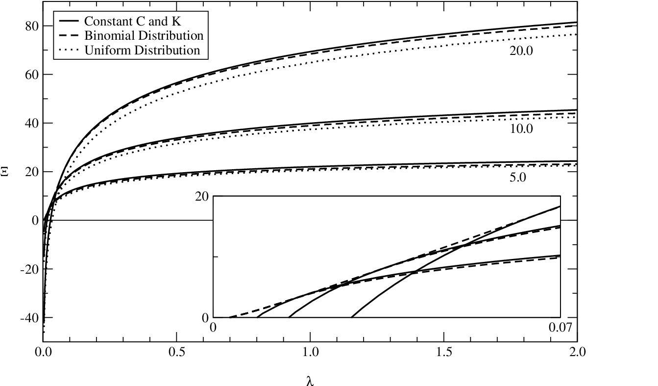
Results for the binomial (dashed line) and uniform (dotted line) distributions with means $\bar{C}=5.0,10.0,20.0$, $q=2$ and $N=300$ are plotted in Fig. 2, together with the value of $\Xi$ with constant $C_{j}=\bar{C}$ and $K_{j}=\bar{C}/\lambda$ values for all $i$ and $j$. This function is explicitly given by

and we can obtain its asymptotic behavior for small and large $\lambda$ as

where $\gamma\approx 0.577216$ is the Euler-Mascheroni constant. Asymptotic limits for large $\lambda$ are given in table 1.

For large $\lambda$ values the result for constant ${\mathbf{C}}$ and ${\mathbf{K}}$ upper-bounds the other two distributions. Additional calculations seem to indicate that it is always the case for any distribution, although a proof for this conjecture is still sought. This implies that if we keep the number of columns constant and increase the ratio $\lambda$ by adding rows, whenever the number of rows is much larger than the number of columns, the average number of matrices becomes independent of both the ratio and number of rows. The plots also suggest that the average number of matrices in these cases are basically defined by the average value of the ${\mathbf{C}}$ distributions.

For small values of $\lambda$, the uniform distribution continues to be upper-bounded by the constant distribution. The binomial distribution, however, is higher for a small interval around zero. This behavior is shown in the inset where lower ${\mathbf{C}}$ values give rise to higher $\Xi$ as $\lambda$ becomes smaller.

Figure 3 shows the results for the Zipf distribution with different values for the power $s$ compared with a uniform distribution in the range $[0,M]$. In this case, the mean of the distributions vary with $\lambda$. We see that, although the average value of the Zipf distributions increasingly differs from the uniform value $M/2$ as $s$ increases, the average number of matrices actually becomes highly similar.

We have introduced a new mapping of Galois matrices to spin systems based on the group homeomorphism between $GF(q)$ under addition mod $q$ (denoted by $\oplus$) and the complex $q$-th roots of unity. In addition, we have introduced a different way for summing over random matrices that can be generalized to include any kind of connectivity constraint and is conceptually cleaner and simpler than the existing approaches. The new mapping and alternative summation over random matrices allows for a factorization of the constraints, which simplifies calculations of the kernel and the number of matrices under various connectivity profiles.

Using the replica approach and these new introduced techniques, we calculated the average dimension of the kernel for a general distribution of non-zero entries and solved the resulting equations numerically, finding that the average kernel density is $1-M/N$ in all cases studied. We conjecture that this result is always valid. Based on the analogy with thermodynamical quantities corresponding to free energy, internal energy and Hamiltonian, we showed that the replica symmetric ansatz in this case must be exact. With the same techniques, we were also able to find the total number of large matrices for fixed ${\mathbf{K}}$ and ${\mathbf{C}}$ and their average number, which was then computed for different distributions of theoretical and practical relevance.

The results presented have practical relevance in a number of areas, including coding network modeling and some biological models. With respect to LDPC codes, the average kernels density result implies that randomly generated LDPC codes typically define codes of rate exactly $1-M/N$, an assumption which is generally made but lacks rigorous derivations. Also, as the parity-parity check matrix can represent the connectivities in graphs (see [17]), the results obtained for the average number of matrices provide a principled approach to determine the average number of possible graphs with a given connectivity distributions of a more general nature than the connectivity profiles examined in this paper.

Support from EPSRC grant EP/E049516/1 is gratefully acknowledged. R.C.A. would also like to thank Dr. Juan P. Neirotti for useful discussions.

References

• [1] R. McEliece, Theory of Information & Coding (Cambridge University Press, Cambridge, MA, 2002 2nd edition).
• [2] K. T. Phelps, J. Rifà, and M. Villanueva, IEEE Trans. Inf. Theory 51, 3931 (2005).
• [3] M. Davey and D. MacKay, IEEE Communications Letters 2, 165 (1998).
• [4] K. Nakamura, Y. Kabashima, and D. Saad, Eurphys. Lett. 56, 610 (2001).
• [5] C. Cooper, Random Structures and Algorithms 16, 209 (2000).
• [6] J. Blömer, R. Karp, and E. Weiz, Random Structures and Algorithms 10, 407 (1998).
• [7] X. Feng and Z. Zhang, Applied Mathematics and Computation 185, 689 (2007).
• [8] M. Mézard, G. Parisi, and M. Virasoro, Spin Glass Theory and Beyond (World Scientific Publishing Co., Singapore, 1987).
• [9] H. Nishimori, Statistical Physics of Spin Glasses and Information Processing (Oxford University Press, Oxford, UK, 2001).
• [10] Y. Kabashima and D. Saad, J. Phys. A. 37, R1 (2004).
• [11] R. Monasson and R. Zecchina, Phys. Rev. Lett. 76, 3881 (1996).
• [12] J. van Mourik and D. Saad, Phys. Rev. E 66, 056120 (2002).
• [13] R. Mulet, A. Pagnani, M. Weigt, and R. Zecchina, Phys. Rev. Lett. 89, 268701 (2002).
• [14] R. C. Alamino and D. Saad, J. Phys A: Math. Theor. 40, 12259 (2007).
• [15] T. Tanaka and D. Saad, Technical report (unpublished).
• [16] B.-Y. Wang and F. Zhang, Discrete Mathematics 187, 211 (1998).
• [17] R. Vicente, D. Saad, and Y. Kabashima, Europhys. Lett. 51, 698 (2000).
• [18] I. S. Gradshteyn and I. M. Ryzhik, in Table of Integrals, Series, and Products, edited by A. Jeffrey and D. Zwillinger (Academic Press, USA, 1993).