Determinant form of modulation equations for the semiclassical focusing Nonlinear Schrödinger equation

The semiclassical analysis of the focusing Nonlinear Schrödinger (NLS)

has produced [2, 3, 4] solutions that one recognizes as modulated multi-phase periodic or quasi-periodic waves. These wave solutions of NLS are expressed in terms of hyperelliptic theta functions (see [1]) built from the radical

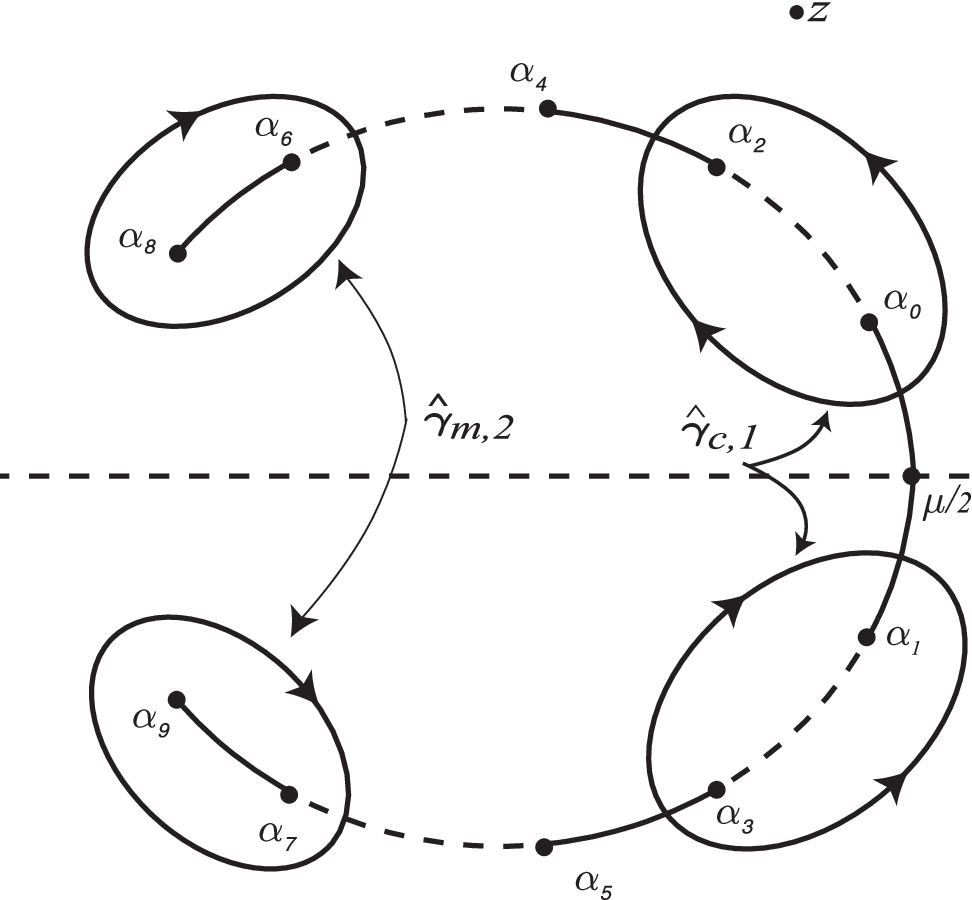
where even $\alpha_{2k}$ lie in the upper halfplane and $\alpha_{2k+1}=\bar{\alpha}_{2k}$. Let $\mathcal{R}=\mathcal{R}(x,t)$ denote the hyperelliptic Riemann surface of $R$, where oriented arcs $\gamma^{+}_{m,k}$, connecting $\alpha_{4k-2}$ and $\alpha_{4k}$, $k=1,2,\cdots,N$, their complex conjugates $\gamma^{-}_{m,k}$, connecting $\alpha_{4k+1}$ and $\alpha_{4k-1}$, together with $\gamma_{m,0}$ connecting $\alpha_{1}$ and $\alpha_{0}$, form the branchcuts (main arcs), see Fig. 1.

Points $\alpha_{i}$ depend on $x,t$ but do not depend on $\varepsilon$. They are called branchpoints of the hyperelliptic Riemann surface $\mathcal{R}$ or simply branchpoints of $R$. The number of wave-phases of a solution $q(x,t,\varepsilon)$ of (1) (in the limit $\varepsilon\rightarrow 0$) is equal to the genus $2N$ of the corresponding Riemann surface $\mathcal{R}(x,t)$. The branchpoints satisfy a system of equations known as the modulation equations or the modulation system that is discussed below.

Nonlinear Schrödinger equation is one of the most celebrated examples of an integrable PDE, i.e., a nonlinear PDE that can be “linearized” through the Lax pair. The “$x$” (spatial) part of the Lax pair is a second order system of linear ODEs

known as Zakharov-Shabat system (see [5]). In the limit $\varepsilon\rightarrow 0$ (semiclassical limit of the NLS) system (3) becomes a singularly perturbed system, and, as such, is a subject of the WKB analysis.

The goal of this paper is to find a determinant formula (see (20)) for the WKB exponential $g$ of (3), to prove its independence of the branchpoints $\alpha$ assuming that $\alpha$ satisfy the modulation equations, and to derive various forms of modulation equations for $\alpha$ using the determinant formula. Our derivation is based on the RHP representation (5) of $g$, which was obtained and discussed in [4] for (1) with pure radiational or radiational and solitons initial data (for the pure soliton case, see [3]). Connection between the WKB exponential $g$ and the RHP (5) is studied in a separate paper [TV2]. The RHP (5) and its solution are the main objects of this paper.

The inverse scattering method of integration of (1) is based on the scattering transform, i.e., on the connection between the initial data of (1) and the scattering data of (3). In general, the scattering data consists of the reflection coefficient defined on $\mathbb{R}$ and of the eigenvalues of Zakharov-Shabat system together with their norming constants (these eigenvalues correspond to solitons). In the semiclassical limit of (1), the reflection coefficient $r_{0}(z,\varepsilon)$ depends on $z$ and $\varepsilon$. We denote

In general, $f$ is a function of $z$ and $\varepsilon$. However, studying the semiclassical limit of (1), we can consider only the leading order term (in $\varepsilon$) of $f$, see [4]. Throughout this paper, we assume that $f(z)$ has analytic continuation into the upper halfplane with the exception of a finite number of logarithmic branchcuts and of isolated singularities. We further assume that the main arcs (branchcuts) of the hyperelliptic surface $\mathcal{R}(x,t)$ do not intersect the singularities of $f(z)$. The values of $f(z)$ in the lower halfplane are obtained by Schwarz reflection. Thus, in general, $\Im f(z)$ has a jump on the real axis.

To define modulation equations, we first assume that the branchpoints $\alpha_{2j}=\alpha_{2j}(x,t)$, $j=0,1,\cdots,2N$, are known. Let $\gamma^{\pm}_{c,k}$ be oriented arcs connecting $\alpha_{4k-4},\alpha_{4k-2}$ and $\alpha_{4k-1},\alpha_{4k-3}$ respectively. These arcs are called complementary arcs. Let $\gamma_{m,k}=\gamma^{+}_{m,k}\cup\gamma^{-}_{m,k}$, $\gamma_{c,k}=\gamma^{+}_{c,k}\cup\gamma^{-}_{c,k}$, $k=1,2,\cdots,N$, where orientation is inherited. Define $g(z)$ as the solution of the RHP:

where all $W_{j},\Omega_{j}$ are some real constants. We assume that the real constant $W_{0}=0$ on the main arc $\gamma_{m,0}$ that connects $\alpha_{1}$ and $\alpha_{0}$.

Let $\gamma$ denote the unioun of all the main arcs $\gamma_{m,j}$, $j=0,1,\cdots,N$ and all the complementary arcs with the inhereted orientation. It is well known that solution to the RHP (5) is given by

Expressing the integrals over the arcs as integrals over the loops shown in Fig. 2, we obtain

where the loops $\hat{\gamma}$ and $\hat{\gamma}_{m,i}$ and the contours $\hat{\gamma}_{c,i}$ ($\hat{\gamma}_{c,i}$ consists of the sum of two arcs oriented oppositely as in the figure) are contractible to their corresponding arcs without passing through $z$.

Deforming $\hat{\gamma}$ so that now $z$ is inside the loop $\gamma$ and still outside the loops $\hat{\gamma}_{m,i}$ and $\hat{\gamma}_{c,i}$, we obtain

where

The function $h(z)$ is obtained by multiplying $g$ by a factor of $2$ and the residue $-f$ being picked up as $z$ cuts through the loop $\hat{\gamma}$.

If $z$ approaches the $i$th main arc from either side, a residue is generated as $z$ cuts through the loop $\gamma_{m,i}$ encircling the arc; multiplied by the factor ${{R(z)}\over{2\pi i}}$ outside the integral, the residue yields the contribution $W_{i}$ to $h$. Similarly, if $z$ approaches the $i$th complementary arc, the contribution to $h$ from $z$ cutting the contour $\gamma_{c,i}$ is $+\Omega_{i}$ or $-\Omega_{i}$, depending on whether $z$ approaches from the left or right of the contour. These observations lead directly to the jump conditions

To see this, one takes into account the above residue calculations and the fact that the expression in the square brackets in (10) is analytic in a neighborhood of any $\alpha_{j}$ (we are assuming distinct $\alpha_{j}$). From the above, it is clear that at any $\alpha=\alpha_{2j}$

where $\pm$ refers to whether $z$ is left or right of the contour and $W,\Omega$ denote real constants on the main and the complementary arcs, adjacent to $\alpha=\alpha_{2j}$.

According to (9), $g(z)\sim O(z^{2N})$ as $z\rightarrow\infty$. The requirement that $g(z)$ is analytic at $z=\infty$ defines the system of $2N$ linear equations for $W_{j},\Omega_{j}$

Modulation equations comes from the requirement that the $L^{2}$-solution to the RHP (5), i.e., the Cauchy operator in (8), commutes with the differentiation in $z$. The equivalent statement is that at every $\alpha=\alpha_{2j}$ the coefficient $\nu_{1}=0$, so that (15) becomes

Equation (17) implies that the expression in the square brackets in equation (10), let us call it $B(z)$, vanishes at every $\alpha_{2j}$, i.e.

where $\ j=0,1,\cdots,2N$ and $\alpha_{2j}$ is inside the loops around the main and the complementary arcs that are adjacent to $\alpha_{2j}$ but outsisde all other loops $\hat{\gamma}_{m,i}$ and $\hat{\gamma}_{c,k}$. The modulation equations (18) is a system of $2N+1$ complex conditions satisfied by the $2N+1$ complex branchpoints $\alpha_{2j}$, $j=0,1,\cdots,2N$. It is also satisfied by their complex conjugates $\alpha_{2j+1}$.

To simplify the notations, we consider below the case $N=1$. The obtained formulae allow a straightforward generalization to the arbitrary $N\in\mathbb{N}$ case. Let

where $\gamma_{m}=\gamma_{m,1}$ and $\gamma_{c}=\gamma_{c,1}$. It is well known that $D\neq 0$ if all $\alpha_{2j},~j=0,1,2$ are distinct.

Multiplying the first two rows of $K(z)$ by $W=W-1$ and $\Omega=\Omega_{1}$ respectively, adding them to the third row and utilizing (10) and (16), we obtain

where $z$ is inside the loop $\hat{\gamma}$ but outside the loops $\hat{\gamma}_{m},\hat{\gamma}_{c}$. That will be our standard assumption about the location of $z$ for the rest of the paper, unless specified otherwise. It is clear that moving $z$ inside the loops $\hat{\gamma}_{m},\hat{\gamma}_{c}$ would generate residue terms $W$ and $\pm\Omega$ (depending on the direction $z$ crosses the oriented loop $\hat{\gamma}_{c}$) in the right hand side of (20). Combining this fact with (17), we obtain a new form of modulation equations

Lemma 2.1 is the basis for the following theorem.

Since $D$ and $R$ do not explicitly depend on $x,t$, Corollary 2.3 together with (20) imply that

Using (19) and

where $f_{0}(z)=\frac{1}{2}\varepsilon i\ln r_{0}(z)$, we calculate

and

where $z$ is outside the loops $\hat{\gamma}_{m},\hat{\gamma}_{c}$.

It is easy to see that if $z$ is inside loops $\hat{\gamma}_{m},\hat{\gamma}_{c}$ the $\hat{\gamma}_{m}$ integrals in (37), (38) are equal to the corresponding integrals on the segment $[\bar{\alpha}_{0},\alpha_{0}]$ multiplied by $-2$, and $\hat{\gamma}_{c}$ integrals in (37), (38) are equal to the corresponding integrals on the segment $[\bar{\alpha}_{4},\alpha_{4}]$ multiplied by $2$. If $z$ is outside any of the loops $\hat{\gamma}_{m},\hat{\gamma}_{c}$, then the corresponding residues should be taken into account.

Modulation equations (21) can be rewritten as ODEs

where $\alpha$ denotes the vector $\alpha=(\alpha_{0},\alpha_{2},\alpha_{4})$ (alternatively, we can consider $\alpha$ to be a 6-dimensional vector). According to (22), in the case $j\neq l$, $j,l=0,2,4$, we have

where $z$ is inside any of the loops $\hat{\gamma}_{m},\hat{\gamma}_{c}$ that surround $\alpha_{m}$. Then $\lim_{z\rightarrow\alpha_{l}}\frac{h(z)}{R(z)}=0$. So, $\frac{\partial K(\alpha_{l})}{\partial\alpha_{j}}=0$. That means that the matrix $\frac{\partial K}{\partial\alpha}$ is diagonal.

To calculate $\frac{\partial K(\alpha_{j})}{\partial\alpha_{j}}$, we notice that

Let us take $j=2$. Then

Equation (17) in a vicinity of $z=\alpha_{2}$ can be rewritten as

where $c_{2}\in\mathbb{C}$. If $z$ is inside any loops $\hat{\gamma}_{m},\hat{\gamma}_{c}$, the constants $W,\Omega$ in (44) should be replaced by zeroes, so we have

Differentiating (45) and taking into the account (10), we obtain

Thus,

Formulae (42)-(48) are also applicable for $\alpha_{0}$, $\alpha_{4}$, if formulae (42), (44), (46) contain only integrals over the loops that are adjasent to $\alpha_{0}$, $\alpha_{4}$ respectively, and only the constants $W,\Omega$ that correspond to these loops.

According to (42)-(48), (39) can be written as

Ordinary differential equations (49) imply

where, according to (37), (38)

This is the Riemann invariant form of modualtion equations written as PDEs.

Alternatively, diffrential form of the modulation equations (49) can be obtained by differentiating (44) and the corresponding equations at $\alpha_{0},\alpha_{2}$. At $\alpha_{2}$ we have

Moving $z$ inside any loops $\hat{\gamma}_{m},\hat{\gamma}_{c}$ that surround $\alpha_{2}$ will eliminate derivatives of $W,\Omega$ in (52). According to (35), (37) and (38), these derivatives are

and

Now equations (49) follows from (52) and (35). Equations (54)-(55) also imply

Finally, since the Cauchy operator for the RHP (5) commutes with differentiation, we have

Combining this with (44) yield $h^{\prime}(z)=\left[\frac{3}{2}c_{j}+O(\sqrt{z-\alpha_{j}}\right]R(z)$ in a vicinity of $z=\alpha_{j}$. Thus,

References

• [1] L.D. Faddeev and L.A. Takhtajan. Hamiltonian Methods in the Theory of Solitons. Springer-Verlag, 1987.
• [2] P. D. Miller; S. Kamvissis. On the semiclassical limit of the focusing nonlinear schr�dinger equation. Phys. Lett. A, 247(1-2):75 –86, 1998.
• [3] S. Kamvissis, K. T.-R. McLaughlin, and P.D. Miller. Semiclassical soliton ensembles for the focusing nonlinear schrödinger equation. Annals of Mathematics Studies 154, Princeton Unversity Press, 2003.
• [4] A. Tovbis, S. Venakides, and X. Zhou. On semiclassical (zero dispersion limit) solutions of the focusing nonlinear schroedinger equation. Comm. Pure Appl. Math, 57(7):877–985, 2004.
• [5] V. E. Zakharov and A. B. Shabat. Exact theory of two-dimensional self-focusing and one-dimensional self-modulation of waves in nonlinear media. Soviet Physics JETP, 34(1):62–69, 1972.