Electronic transport in inhomogeneous quantum wires

Our starting point is a one-dimensional system of weakly interacting electrons with spins. In order to account for a non-uniform electron density $n(x)$, we introduce a one-particle potential $U(x)$ originating from the surrounding gates and impurities in the substrate. Moreover, the interaction between electrons is inhomogeneous, and described by a smoothly varying potential $V(r,R)$, given in the center-of-mass coordinates. The Hamiltonian for this system takes the form

where $\psi^{\dagger}_{\gamma}(x)$ creates an electron with spin projection $\gamma$ at position $x$, and $\mu$ is the chemical potential. We assume that the potential $U(x)$ is a smooth function of position, and that $U(x)\ll\mu$. This allows us to introduce a position-dependent Fermi energy $\epsilon_{F}(x)=\mu-U(x)$. Similarly, the position-dependent Fermi momentum and velocity are straightforwardly defined as $p_{F}(x)=\sqrt{2m\epsilon_{F}(x)}$ and $v_{F}(x)=p_{F}(x)/m$.

We keep a very general form for the interaction potential between electrons and only make the following assumptions concerning its characteristic length scales. On the one hand, we assume for simplicity that the interaction is short-range, the potential decaying rapidly as a function of the distance $r$ between electrons. On the other hand, since we consider a non-uniform system, the interaction depends on the position $R$ of the center of mass. The variations with respect to $R$ are smooth and occur at a typical length scale $d$, large compared to both the Fermi wavelength and the range of the interaction potential. Similarly, we assume that the potential $U(x)$ varies at the same typical length scale $d$ as the interaction strength.

We focus now on temperatures in a broad range $\hbar v_{F}/d\ll T\ll\epsilon_{F}$. In order to compute the resistivity of the wire, we consider a force balance on a small isolated segment of wire taken at position $x$, whose length $\Delta x$ well exceeds the range of the interaction while satisfying $\hbar v_{F}/T\ll\Delta x\ll d$. When an external current $I$ is applied to the device, the response of the system manifests itself as a local electric field $E(x)=\rho(x)I$, which in turn leads to a driving force $eE(x)n(x)\Delta x$ acting on the electrons. This driving force is compensated by a damping force $\Delta F$ resulting from the inhomogeneous electron-electron interaction, so that the resistivity can be written as

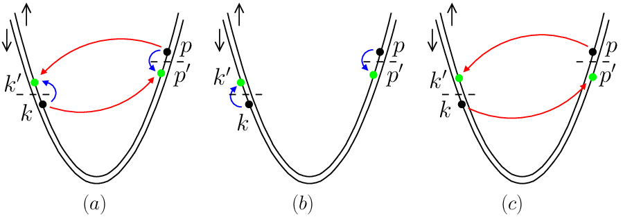
The damping force can be evaluated as the change in momentum per unit time associated with two-particle scattering processes. In the regime $k_{F}d\gg 1$, the processes with a large momentum difference compared with the Fermi momentum lead to exponentially small contributions. As a result, in what follows we focus on processes which only weakly violate the momentum conservation (see figure 2).

Because of the non-uniformity of the wire, strictly speaking the momentum of the electron is not a well-defined quantity. However, since $U(x)$ varies smoothly over a length scale $d\gg\Delta x$, it is possible to introduce a well-defined momentum over the size of the small segment under consideration. The expression for the momentum thus depends on the position $x$ of the small segment, and for a state of energy $\epsilon$ is given by $p_{\epsilon}(x)=\pm\sqrt{2m\left[\epsilon-U(x)\right]}$. Here the $+$ sign corresponds to the right branch, the $-$ sign to the left one.

Similarly, the eigenstates of the free Hamiltonian are no longer given by simple plane waves but instead satisfy $\left[-\hbar^{2}\partial_{x}^{2}/2m+U(x)\right]\Psi_{\epsilon}(x)=\epsilon\Psi_{\epsilon}(x)$. Keeping in mind that the typical length scale $d$ associated with the inhomogeneities of the wire is much larger than the Fermi wavelength, we use the semiclassical approximation, which yields

normalized according to $\int\rmd x\Psi_{\epsilon,\pm}(x)\Psi_{\epsilon^{\prime},\pm}^{*}(x)=2\pi\delta(\epsilon-\epsilon^{\prime})$. Here the velocity is defined as $v_{\epsilon}(x)=p_{\epsilon}(x)/m$ and the index $\pm$ refers to the right/left branches. We ignored the backscattered wave, since it only leads to exponentially small contributions for $k_{F}d\gg 1$.

The rate of change of momentum associated with the three processes shown in figure 2 is evaluated using the Fermi golden rule, so that the damping force acting on the electrons takes the form

where we introduced ${V}_{pk;p^{\prime}k^{\prime}}$ as the matrix element of the interacting Hamiltonian (2c) for scattering from the initial state $(p,k)$ to the final state $(p^{\prime},k^{\prime})$ according to the processes shown in figure 2. The superscripts $\parallel$, 2$\perp$ and 1$\perp$ refers to the standard notations for these scattering processes [35]. The occupation numbers $f^{R,L}$ introduced in (2e) are given by the Fermi distribution evaluated with the appropriate temperatures $T_{R,L}(x)$, defined in section 2.

One readily sees from (2e) that the damping force vanishes at $T_{R}=T_{L}$. Using the fact that the temperature difference $T_{R}-T_{L}\propto I$ is small in the linear response regime, we expand the occupation numbers $f^{R,L}$ to first order in $T_{R}-T_{L}$. To avoid redundant derivations, let us focus on the first process shown on figure 2$(a)$. The damping force corresponding to this scattering process is then given by

where we converted the summations over states into energy integrals, and introduced the matrix element $V^{\parallel}\left(\epsilon_{p},\epsilon_{k};\epsilon_{p^{\prime}},\epsilon_{k^{\prime}}\right)$ evaluated using the set of eigenstates defined in (2d).

Note that the expansion in $T_{R}-T_{L}$ leads to an expression for the damping force which is proportional to the applied current. As a result, in the linear response regime we can ignore any further dependence on $I$, as this would lead to contributions that are non-linear in the current bias. This allows us to use the Fermi energy $\epsilon_{F}$ and velocity $v_{F}$ as they are defined in the equilibrium state, i.e. in the reference frame where the electric current vanishes.

Focusing on states close to the Fermi energy, we can simplify the expression for the eigenstates (2d) of the free Hamiltonian into

where $\Psi_{\epsilon_{F},\pm}(x)$ is obtained from (2d) by setting $\epsilon=\epsilon_{F}$. This allows us to estimate the matrix element $V^{\parallel}$ to first order in the interaction:

Here we introduced the Fermi wave vector $k_{F}(R)=p_{F}(R)/\hbar$.

Using the fact that $p$ and $p^{\prime}$ on the one hand, and, $k$ and $k^{\prime}$ on the other hand, are on the same branch, we express the momentum difference in terms of a difference in energy by introducing the density of states. We then define $\varepsilon=\epsilon_{p^{\prime}}-\epsilon_{p}+\epsilon_{k}-\epsilon_{k^{\prime}}$, and perform the remaining energy integrals. Combining the resulting expression for the damping force with (2c), and substituting the matrix element (2h), we obtain the following expression for the resistivity associated with the scattering process of figure 2$(a)$

The shortened notations $V_{0}$ and $V_{2k_{F}}$ correspond to the zero-momentum and $2k_{F}$ Fourier components of the potential $V(r,R)$ with respect to its first variable $r$ defined as:

At this stage, it is convenient to rewrite the energy integral in (2i) by replacing $\varepsilon^{2}$ with a second derivative of the exponential term with respect to $R_{1}$ and $R_{2}$, along with the appropriate factors of $\hbar v_{F}$. Performing an integration by parts in the position variables leaves us with an expression involving single derivatives of the dimensionless parameters $V_{0}(R)/\left[\pi\hbar v_{F}(R)\right]$ and $V_{2k_{F}}(R)/\left[\pi\hbar v_{F}(R)\right]$. The remaining integral over $\varepsilon$ can be easily simplified by noticing that it is the Fourier transform of a rapidly decaying function which only extends over a range of energy comparable to temperature. For temperatures $T\gg\hbar v_{F}/d$, it reduces to a delta function in $R_{1}-R_{2}$ which allows us to simplify (2i) to

where we expanded the remaining position integral to first order in $\Delta x$.

The contributions corresponding to the remaining two scattering processes can be computed following the same steps and are readily obtained from (2k) by replacing $V_{0}(x)-V_{2k_{F}}(x)$ with $V_{0}(x)$ for $\rho_{2\perp}(x)$, and with $V_{2k_{F}}(x)$ for $\rho_{1\perp}(x)$. Combining the contributions from all three processes, the final expression for the resistivity in the regime of temperatures $T\gg\hbar v_{F}/d$ takes the form

This expression clearly stresses that the meaningful inhomogeneous quantity is not just the interaction potential but rather the dimensionless parameter that involves both the electron-electron interaction and the Fermi velocity. In particular, this means that a system with a non-uniform density but homogeneous interactions between electrons still displays a non-zero resistivity.

Previous attempts at studying the transport properties of quantum wires relied on an extension of the Tomonaga-Luttinger model to inhomogeneous systems [18, 19, 20]. These authors assumed that the inhomogeneities do not change the form of the Hamiltonian, and can be accounted for by introducing position-dependent velocities and Luttinger-liquid parameters. In the general case, however, a rigorous derivation of the bosonized Hamiltonian for these systems is still lacking. Here we show how such a bosonized Hamiltonian can be derived explicitly in the case of a non-uniform system of weakly interacting electrons.

The standard bosonization formula for weakly interacting fermions involves the Fermi momentum as well as a momentum cutoff (see e.g. [17]), and as such cannot be straightforwardly extended to non-uniform systems where both these quantities can develop a position dependence. The key idea then is to map the inhomogeneous system of electrons onto a set of fictitious fermions described by a Hamiltonian whose non-interacting part is translationally invariant. From there, a standard bosonization procedure holds and the resulting Hamiltonian expressed in terms of the new variables is very reminiscent of the conjectured inhomogeneous Luttinger liquid Hamiltonian, in the limit of weak interactions (see section 5).

Our starting point is similar to the one we considered in section 3, namely a system of interacting electrons with a non-uniform density described by the Hamiltonian (0). As we noticed in the previous section, the non-uniform potential $U(x)$ appearing in (2b) breaks the translational invariance of the system, already when no electron-electron interaction is present. As a result, the eigenstates of the free Hamiltonian are no longer plane waves but for energies close to the Fermi level, they can be approximated by (2g).

Up to a prefactor which depends on position but not on $\epsilon$, these low-energy eigenstates look like plane waves, putting forth a more natural set of variables: the energy difference $\epsilon-\epsilon_{F}$ and $X(x)=\int_{0}^{x}\rmd x^{\prime}/\hbar v_{F}(x^{\prime})$. An expansion of the electron field operator $\psi_{\gamma,\pm}(x)$ over these plane waves calls for the introduction of a fictitious fermion field operator $\eta_{\gamma,\pm}(X)$ defined as

where $\Psi_{\epsilon_{F},\pm}(x)$ was introduced in (2g). Note that the anti-commutation relations satisfied by $\psi_{\gamma,\pm}(x)$ transfer to $\eta_{\gamma,\pm}(X)$ ensuring that $\left\{\eta_{\gamma,\sigma}(X),\eta_{\beta,\sigma^{\prime}}^{\dagger}(Y)\right\}=\delta_{\sigma\sigma^{\prime}}\delta_{\gamma\beta}\delta(X-Y)$.

Let us now derive the Hamiltonian describing the physics of these fictitious fermions. This is accomplished by substituting (2m) into the Hamiltonian (0). By construction, the free Hamiltonian is translationally invariant in the new variable $X$. At low energy, the interacting part of the Hamiltonian can be decomposed in three sectors corresponding to the conventional $g_{1}$, $g_{2}$ and $g_{4}$ processes [35]. The main difference here is that the associated coupling constants are now position-dependent. They can be obtained from the Fourier components of the electron-electron interaction potential.

As an example, consider the so-called $g_{2\parallel}$ process. Following [17], the coupling constant for this process is given by the zero-momentum Fourier component of the interaction potential, which in the case of our inhomogeneous system corresponds to $V_{0}(x)$, introduced in (2j). Replacing $\psi$ with $\eta$ according to (2m), and introducing the density operator $\nu_{\gamma,\pm}(X)=\eta_{\gamma,\pm}^{\dagger}(X)\eta_{\gamma,\pm}(X)$, the $g_{2\parallel}$ process retains the same form

only with a dimensionless coupling constant given by $y_{2\parallel}\left(X(x)\right)=g_{2\parallel}(x)/\pi\hbar v_{F}(x)$. A similar treatment can be applied to the remaining sectors of the interaction.

The resulting Hamiltonian expressed in terms of the fictitious field $\eta$ can now be bosonized following the standard procedure:

where we introduced the fields $\phi_{\nu}$ and $\theta_{\nu}$ (with $\nu=\rho,\sigma$) satisfying bosonic commutation relations $\left[\phi_{\nu}(X),\partial_{Y}\theta_{\nu}(Y)\right]=\rmi\pi\delta(X-Y)$. Here $U_{\gamma,\pm}$ are the standard Klein factors [17] and $\alpha^{-1}$ is an energy cutoff¹¹ 1 Considering that the fictitious fermions were introduced in the vicinity of the electron Fermi surface, one should assume $\alpha^{-1}\ll\epsilon_{F}$. introduced to regularize the theory in the ultra-violet sector.

In terms of the bosonic variables, the Hamiltonian of the system can be written as a sum of two terms describing the excitations of charge and spin degrees of freedom respectively, and takes the form

The dimensionless parameters $y_{\rho}$ and $y_{\sigma}$ are conventional notations for combinations of $y_{1}$, $y_{2}$ and $y_{4}$ [17] given by

where $V_{0}$ and $V_{2k_{F}}$ are the Fourier components of the interaction potential as defined in (2j).

Note that this form of bosonization clearly highlights that the important variables are the dimensionless parameters $y_{\rho,\sigma}$ rather than the various interaction constants $g_{1,2,4}$. The calculation of the resistivity carried out in section 3 led to the same observation, see (2l).

A way to determine the resistivity of the system is to relate it to the mechanism of dissipation of energy into the wire when an external current bias is applied. This relation was explored in [36] in the context of a quantum wire in the Wigner crystal regime, and the method we outline here is similar.

In the presence of an applied current $I=I_{0}\cos\omega t$, the electrons start moving in the wire. More specifically, in the dc limit $\omega\to 0$, one can assume that the current is uniform throughout the wire and all electrons move in phase. As a result, the position of the electrons depends on time and is related to the injected charge $q(t)=I_{0}\omega^{-1}\sin\omega t$ defined as $I(t)=\dot{q}(t)$. This time dependence of the positions of the electrons can be accounted for by replacing $x\to x+q(t)/en(x)$ in the position-dependent parameters of the Hamiltonian. While this has no effect in practice when the translational invariance holds, for an inhomogeneous system it leads to a time-dependent perturbation to the Hamiltonian. Alternatively, this amounts to describing the system in the reference frame moving with the electron fluid. In this case, the electrons experience the effect of an inhomogeneous potential moving as a function of time.

In terms of the fictitious set of fermions $\eta_{\gamma,\pm}(X)$, one needs to substitute $X$ in the dimensionless interaction parameters $y_{\rho,\sigma}$ by the time-dependent position $X+q(t)/en(X)$ where the density in these variables is given by $n(X(x))=n(x)\hbar v_{F}(x)$. In the linear response regime, an expansion to first order in $q(t)$ leads to the following form of the Hamiltonian:

where we introduced the notation ${\cal H}^{\prime}(X)={\cal H}_{\rho}^{\prime}(X)+{\cal H}_{\sigma}^{\prime}(X)$ for the following quantities:

The time-dependent perturbation in (2opr) acts as an external driving force, resulting in the creation of spin and charge excitations. These excitations are responsible for dissipating the energy from the external force into the wire. Using the Fermi golden rule, it is possible to estimate the rates of these absorption and emission processes, and therefore, the energy $W$ dissipated in unit time into the system. In the linear response regime, where the amplitude $I_{0}$ of the current oscillations is weak, the energy dissipated in unit time is quadratic in $I_{0}$ and is given by

where $\langle\ldots\rangle$ stands for thermodynamic averaging.

The resistance of the system is then derived by comparing the dissipated energy obtained in (2opst) with the Joule heat law $W=I_{0}^{2}R/2$. Since the charge part (2opsa) and the spin part (2opsb) of the time-dependent perturbation commute, one expects the resistance $R$ of the wire to be expressed as the sum of a spin and a charge contribution $R=R_{\rho}+R_{\sigma}$, which can be evaluated separately. This can be understood as the consequence of having two independent channels for dissipating energy throughout the wire, corresponding to spin and charge excitations [36]. After some manipulations, these two contributions to the resistance can be expressed in the dc limit as

Here we introduced the retarded correlator ${\cal W}_{{\rm ret},\nu}$ as the Fourier transform in time of ${\cal W}_{{\rm ret},\nu}(X,Y;t)=-\rmi\theta(t)\langle\left[{\cal H}_{\nu}^{\prime}(X,t),{\cal H}_{\nu}^{\prime}(Y,0)\right]\rangle$, where $\nu=\rho,\sigma$.

In order to derive the contribution to the resistivity from charge degrees of freedom, we substitute in (2opsu) the expression for ${\cal H}_{\rho}^{\prime}$ introduced in (2opsa). The retarded correlator ${\cal W}_{{\rm ret},\rho}$ resulting from this substitution is quartic in the bosonic field $\phi_{\rho}$. It is thus more convenient to express it in terms of the corresponding time-ordered correlation function, via an analytic continuation in frequency space. This allows for the use of Wick’s theorem, ultimately leading to the following expression of the retarded correlator:

where $\langle T\ldots\rangle$ corresponds to the time-ordered correlation function.

Since (2opsv) is explicitly quadratic in the interaction, the dominant contribution to the retarded correlator ${\cal W}_{{\rm ret},\rho}$ can be derived by using the free propagator of the bosonic field $\phi_{\rho}$. The latter is readily obtained from the non-interacting Hamiltonian, and is given by

Combining (2opsw) with (2opsv), performing the integral over imaginary time $\tau$, and substituting the analytically continued result into (2opsu), the charge contribution to the resistance in the dc limit reads:

where we restricted ourselves to contributions up to second order in the interaction.

One recognizes in (2opsx) a rapidly decaying integral kernel for $|X-Y|\gg 1/T$. In terms of real space quantities, this corresponds to distances of order $\hbar v_{F}/T$. It follows that at temperatures $T\gg\hbar v_{F}/d$ the double integral in $X$ and $Y$ is dominated by short-range contributions. This allows us to reduce the expression (2opsx) for the resistance to a single integral over $X$. Changing variables back from $X$ to $x$, the integrand of the resulting expression for the resistance $R_{\rho}$ can be identified with the charge contribution to the resistivity at position $x$ in space and is given by

where we focused on temperatures in the range $\hbar v_{F}/d\ll T\ll\epsilon_{F}$.

The method used above to derive the charge contribution to the resistivity can be readily extended to evaluate that of spin degrees of freedom. Substituting the expression for ${\cal H}_{\sigma}^{\prime}$ into (2opsu), one notices that the spin contribution splits off into two parts: one coming from the quadratic term in $\phi_{\sigma}$, the other from the cosine term.

It is interesting to compare the bosonized Hamiltonian we derived in (0) to that of the inhomogeneous Tomonaga-Luttinger model conjectured in [18, 19, 20]. To do so, we change variables back from $X$ to $x$, so that the Hamiltonian (0) takes the form

where we denoted $\varphi_{\nu}(x)=\phi_{\nu}(X(x))$ and $\vartheta_{\nu}(x)=\theta_{\nu}(X(x))$ (with $\nu=\rho,\sigma$).

The charge Hamiltonian $H_{\rho}$ and the quadratic part of $H_{\sigma}$ are identical to the inhomogeneous Tomonaga-Luttinger Hamiltonian [18, 19, 20], taken in the limit of weak interactions. The important difference comes from the cosine term of the spin Hamiltonian. This term was absent from previous works which either discarded it arguing that the coupling constant $g_{\sigma}$ renormalizes towards zero at low energy scales [37], or simply focused on a system of spinless fermions [18, 19, 20]. To recover a standard form for the cosine term, one needs to introduce a position-dependent momentum cutoff $\left[\alpha(x)\right]^{-1}$ defined as $\alpha(x)=\alpha\hbar v_{F}(x)$, where $\alpha^{-1}$ is the energy cutoff introduced in (0). Keeping in mind that momentum is no longer a conserved quantity in our model, this position dependence of the momentum cutoff was to be expected. Interestingly though, the natural guess relying on the common interpretation of $\alpha(x)$ as a small distance cutoff, would have led to a different answer. Indeed, assuming that $\alpha(x)$ represents the shortest inter-particle distance, one would expect it to be inversely proportional to the electron density, i.e. $\alpha(x)\propto 1/v_{F}(x)$.

Although the quadratic part of our bosonized Hamiltonian is similar to the model considered [18, 19, 20], we do not reach the same final answer. This is because our treatment amounts to considering perturbations to the Luttinger-liquid Hamiltonian which were not taken into account in previous studies. In section 4, we treated $I(t)$ as an external parameter. In the framework of the Luttinger liquid model, it can also be interpreted as an excitation of the charge mode. Using the bosonization expression for the electric current $I=e(\sqrt{2}/\pi)\dot{\phi_{\rho}}$, one readily sees that $q(t)$ can thus appear as a dynamical variable, directly proportional to the charge field $\phi_{\rho}$. As a result, the linear in $q(t)$ perturbation to the Hamiltonian in (2opr) corresponds, in the conventional Luttinger-liquid theory, to cubic terms in the bosonic fields of the form $\phi_{\rho}(\partial_{X}\phi_{\nu})^{2}$ ($\nu=\rho,\sigma$). These terms are irrelevant perturbations to the Luttinger-liquid Hamiltonian, and as such are usually discarded. However, it was proven that within the quadratic Luttinger-liquid Hamiltonian, non-uniform electron-electron interactions do not contribute to the resistance [18, 19, 20]. It thus makes sense to take these irrelevant perturbations into account. Our approach showed that they affect the transport properties in a non-trivial way and lead to a finite resistivity.

Our results are relevant to experiments performed on long quantum wires. However, we focused on the case of weakly interacting electrons which is unlikely to be realized in experimental situations. Let us discuss to what extent our conclusions are modified when this restriction on the interaction strength is relaxed.

Though our results are not readily applicable in the case of strong electron-electron interactions, the method developed in section 4 which relies on bosonization suggests that the temperature and density dependences of the resistivity should not be affected by the strength of the interactions. Experimental measurements of these dependences may thus be compared with our results.

Furthermore, given the Hamiltonian of the system in the strongly interacting regime, one could repeat the treatment of section 4 in order to derive the resistivity. Unfortunately, a rigorous derivation of the bosonized Hamiltonian in the case of a strongly interacting inhomogeneous system is yet to be found.

In our derivation, we assumed that the electronic subsystem is in equilibrium in the moving frame. For this to be satisfied, we need the wires to be longer than the typical length scale $l_{\rm eq}$ associated with the processes of equilibration taking place inside the wire. If the size of the wire becomes too short with respect to the equilibration length $l_{\rm eq}$, we expect our results to be modified by an additional small prefactor of the order of the ratio of these two length scales. This might lead to a non-trivial temperature dependence of the resistance, depending on the leading equilibration mechanism involved.

Little is known about equilibration mechanisms in one-dimensional interacting systems. In the case of weakly interacting electrons, recent work [34] suggests that scattering processes involving three electrons may be the leading source of equilibration in the system. Because of consideration of energy and momentum conservation, these three-particle collisions should involve states near the bottom of the band, resulting in a strong suppression at low temperatures. In the experimentally relevant case of low electron density and strong interactions, this analysis no longer holds and a detailed treatment remains elusive. It is natural to expect that the equilibration in the wire would become easier as the interactions grow stronger.

References

- [1] van Wees B J, van Houten H, Beenakker C W J, Williamson J G, Kouwenhoven L P, van der Marel D and Foxon C T 1988 Phys. Rev. Lett. 60 848
- [2] Wharam D A, Thornton T J, Newbury R, Pepper M, Ahmed H, Frost J E F, Hasko D G, Peacock D C, Ritchie D A and Jones G A C 1988 J. Phys. C: Solid State Phys. 21 L209
- [3] Thomas K J, Nicholls J T, Simmons M Y, Pepper M, Mace D R and Ritchie D A 1996 Phys. Rev. Lett. 77 135
- [4] Thomas K J, Nicholls J T, Appleyard M J, Simmons M Y, Pepper M, Mace D R and Ritchie D A 1998 Phys. Rev.B 58 4846
- [5] Thomas K J, Nicholls J T, Pepper M, Tribe W R, Simmons M Y and Ritchie D A 2000 Phys. Rev.B 61 R13365
- [6] Kristensen A et al. 2000 Phys. Rev.B 62 10950
- [7] Reilly D J et al. 2001 Phys. Rev.B 63 R121311
- [8] Cronenwett S M, Lynch H J, Goldhaber-Gordon D, Kouwenhoven L P, Marcus C M, Hirose K, Wingreen N S, and Umansky V 2002 Phys. Rev. Lett. 88 226805
- [9] de Picciotto R, Pfeiffer L N, Baldwin K W and West K W 2005 Phys. Rev.B 72 033319
- [10] Rokhinson L P, Pfeiffer L N and West K W 2006 Phys. Rev. Lett. 96 156602
- [11] Crook R, Prance J, Thomas K J, Chorley S J, Farrer I, Ritchie D A, Pepper M and Smith C G 2006 Science 312 1359
- [12] Bockrath M, Cobden D H, Lu J, Rinzler A G, Smalley R E, Balents L and McEuen P L 1999 Nature 397 598
- [13] Auslaender O M, Yacoby A, de Picciotto R, Baldwin K W, Pfeiffer L N and West K W 2000 Phys. Rev. Lett. 84 1764
- [14] Yao Z, Postma H W C, Balents L and Dekker C 1999 Nature 402 273
- [15] Auslaender O M, Steinberg H, Yacoby A, Tserkovnyak Y, Halperin B I, Baldwin K W, Pfeiffer L N and West K W 2005 Science 308 88
- [16] Haldane F D M 1981 J. Phys. C: Solid State Phys. 14 2585
- [17] Giamarchi T 2004 Quantum Physics in One Dimension (Oxford University Press)
- [18] Maslov D L and Stone M 1995 Phys. Rev.B 52 R5539
- [19] Safi I and Schulz H J 1995 Phys. Rev.B 52 R17040
- [20] Ponomarenko V V 1995 Phys. Rev.B 52 R8666
- [21] Wang C K and Berggren K F, Phys. Rev. B 54 R14257 (1996)
- [22] Spivak B and Zhou F 2000 Phys. Rev.B 61 16730
- [23] Meir Y, Hirose K and Wingreen N S 2002 Phys. Rev. Lett. 89 196802
- [24] Rejec T and Meir Y 2006 Nature 442 900
- [25] Bruus H and Flensberg K 1998 Semicond. Sci. Technol. 13 A30
- [26] Tokura Y and Khaetskii A 2002 Physica E 12 711
- [27] Seelig G and Matveev K A 2003 Phys. Rev. Lett. 90 176804
- [28] Meidan D and Oreg Y 2005 Phys. Rev.B 72 121312
- [29] Syljuasen O F 2007 Phys. Rev. Lett. 98 166401
- [30] Sloggett C, Milstein A I and Sushkov O P 2006 Correlated electron current and temperature dependence of the conductance of quantum point contact Preprint arXiv:cond-mat/0606649
- [31] Lunde A M, De Martino A, Egger R and Flensberg K 2007 Electron-electron interaction effects in quantum point contacts Preprint arXiv:0707.1989
- [32] Rech J and Matveev K A 2008 Phys. Rev. Lett. 100 066407
- [33] Pustilnik M, Mishchenko E G, Glazman L I and Andreev A V 2003 Phys. Rev. Lett. 91 126805
- [34] Lunde A M, Flensberg K and Glazman L I 2007 Phys. Rev.B 75 245418
- [35] Sólyom J 1979 Adv. Phys. 28 209
- [36] Matveev K A 2004 Phys. Rev.B 70 245319
- [37] Safi I and Schulz H J 1999 Phys. Rev.B 59 3040