DESY-07-154, CERN-PH-TH/2008-048
Phases Of Theories In Dimensions With Boundary
Manfred Herbst, Kentaro Hori and David Page
Theory Division, Department of Physics, CERN, CH–1211 Geneva 23, Switzerland
Department of Physics, University of Toronto, 60 St. George Street, Toronto, Ontario, M5S 1A7, Canada
We study B-type D-branes in linear sigma models with Abelian gauge groups. The most important finding is the grade restriction rule. It classifies representations of the gauge group on the Chan-Paton factor, which can be used to define a family of D-branes over a region of the Kähler moduli space that connects special points of different character. As an application, we find a precise, transparent relation between D-branes in various geometric phases as well as free orbifold and Landau-Ginzburg points. The result reproduces and unifies many of the earlier mathematical results on equivalences of D-brane categories, including the McKay correspondence and Orlov’s construction.
March, 2008
Notation
The time coordinate of the worldsheet is denoted and the space coordinate is , except in Section 6 where we use for the space coordinate. Light cone coordinates are and their derivatives are . The worldsheet itself is denoted as . Supercharges are denoted by bold face . For example, generators are , . On the other hand, is used for the holomorphic part of an open string tachyon profile.
1 Introduction
D-branes in Calabi-Yau manifolds play central roles in string theory and related fields. They can be used to construct and study models of particle physics and cosmology with spontaneously broken or unbroken supersymmetry. They also determine extremal black holes in four-dimensional supergravity or BPS states in field theory. A lot of efforts have been devoted to this subject in the past twelve years. Most are done in large volume regimes where the corrections are small or negligible and the ten-dimensional supergravity can be used. There are also studies of D-branes at special non-geometric backgrounds with exactly solvable worldsheet conformal field theories, such as Gepner models and free orbifolds. Furthermore, some works probe singular points of the moduli space where the worldsheet description breaks down. Although there are still many things to be understood, a body of solid knowledge is accumulating at special points of the moduli space where convenient descriptions of the theory are available.
A natural and important problem is to connect the information at the special points and to obtain a global picture of D-branes over the entire moduli space of backgrounds. For example, this will be necessary to understand the totality of vacua. Some quantities are protected from quantum corrections and are either constant or holomorphic as functions of the moduli fields. For those, we may be able to glue together the information at special points trivially or by analytic continuation. Ramond-Ramond (RR) charges of D-branes are good examples — the connection between large volume regimes and Gepner points was successfully found in the seminal paper [3]. However, most quantities do not possess such properties. We would like to have at least some hint to study the vast unexplored regions.
For closed strings, linear sigma models [4] provide an ultra-violet description of the worldsheet theories over the entire moduli space in a large class of examples. They were used to find a simple and global picture of the stringy moduli space that had been available only via mirror symmetry, and they had also been used to derive mirror symmetry itself. A natural idea is to use them also to study D-branes. The main goal of the present paper is to construct an ultra-violet description of the worldsheet theory with boundary, using linear sigma models, that is valid in regions of the moduli space that encompass various special points of different character. Just as in the bulk theories, we would like to have a workable method of construction which is very explicit and transparent.
To be precise our focus will be on the description of B-type D-branes over the bulk of the Kähler moduli space. The moduli space of superconformal field theories is a product of two spaces, and , which are referred to as the “complex structure moduli space” and the “Kähler moduli space” according to their interpretation in large volume regimes. It is the Kähler moduli space that has special points with various different descriptions. Relevant D-branes are those preserving a half of the supersymmetry, and there are two types: A-branes and B-branes. In a large volume regime, A-branes are wrapped on Lagrangian submanifolds and B-branes are wrapped on complex submanifolds. They have chiral sectors that are protected from renormalization. The chiral sector of B-branes depends holomorphically on and is invariant under deformations in . Correspondingly, the tree-level spacetime superpotential depends holomorphically on the complex structure moduli fields but is independent of the Kähler moduli fields. Note that this does not mean that B-branes do not depend at all on . The spacetime D-term potential and stability of the branes depend primarily on the Kähler moduli. These facts make it feasible and yet interesting to study B-branes over the Kähler moduli space.
Linear sigma models are a simple class of (2,2) supersymmetric gauge theories. In this paper, we only consider models with Abelian gauge groups. Fayet-Iliopoulos (FI) parameters enter into the worldsheet D-term equations and determine the pattern of gauge symmetry breaking and massless fields. The pattern decomposes the space of FI parameters into domains called “phases”. On a “phase boundary”, there is a classical vacuum configuration with an unbroken continuous subgroup which is generically a . The quantum gauge theory also depends on the theta angles, which are interpreted as the background electric fields. The Kähler moduli space is thus spanned by the FI parameters as well as the theta angles.
A part of the data to specify a D-brane in a linear sigma model is the representation of the gauge group on the Chan-Paton space, that is, the charges of the Chan-Paton vectors. The most important result of the present paper is the grade (or band) restriction rule. It provides the necessary and sufficient condition so that a “parallel family” of D-branes can be defined over a region of the moduli space which covers two adjacent phases and their phase boundary. The condition is on the Chan-Paton charges of the brane with respect to the unbroken subgroup at the phase boundary, and goes as follows. Let be the sum of all positive charges under that of the bulk matter fields. Then the condition on the Chan-Paton charge is that
| (1.1) |
for any value of at the phase boundary in the region of under consideration.
The present work is strongly motivated by recent developments in mathematics. The D-brane category, which has the same information as the chiral sector of all possible boundary interactions in a fixed bulk theory, provides active areas of research in algebraic geometry and symplectic geometry, after M. Kontsevich’s homological mirror symmetry conjecture [5]. The category of B-branes in a large volume regime is the derived category of the target space, while in an orbifold theory it is the derived category of objects with orbifold group action. In a Landau-Ginzburg model it is the category of matrix factorizations of the superpotential. The categories of B-branes of bulk theories that are related by Kähler deformations must be equivalent, as a consequence of the invariance of the chiral sector. Mathematically, an equivalence of categories is given by a pair of maps of objects and morphisms with certain isomorphism conditions. Recently, such equivalences of D-brane categories were constructed. One example is the categorical version of McKay correspondence [6], that is, the equivalence of the derived category of a non-compact toric Calabi-Yau manifold and the derived category for the orbifold theory which sits at a different point of the same Kähler moduli space. Also, D. Orlov constructed equivalences between the derived category of the Calabi-Yau hypersurface defined by a polynomial and the category of matrix factorizations of the same polynomial [7]. A natural question is whether these equivalences are the ones relevant for physics. Our work grew out of an attempt to answer this question.
The organization of the rest of the paper is as follows.
In Section 2, we describe B-type D-branes in non-linear sigma models, Landau-Ginzburg models, and their orbifolds. We determine the condition of supersymmetry and R-symmetry on the invariant boundary interactions given by Quillen’s superconnections. This leads to complexes of vector bundles as the data of D-branes in non-linear sigma models and homogeneous matrix factorizations of the superpotential for Landau-Ginzburg models. We also study the chiral sector of each system and describe the corresponding D-brane category.
In Section 3, we look into D-term deformations and brane-antibrane annihilation, which are operations that do not change the low energy behaviour of the boundary interactions. We show that a quasi-isomorphism between complexes of vector bundles can be obtained by a chain of D-term deformations and brane-antibrane annihilation. This clarifies the relevance of quasi-isomorphisms in brane-antibrane systems, which was discussed earlier in [8] from the spacetime point of view. We also study relevant and marginal deformations of the bulk theory. We study what happens to D-branes when a pair of bulk fields with F-term mass are integrated out, and find the map of D-branes from the high energy theory to the low energy theory (we call it Knörrer’s map). We end the section with the study of marginal Kähler deformations which is the main subject of this paper. We determine the rule of D-brane transport along a path in the Kähler moduli space, and show that it defines the notion of a “flat connection” for the “bundle” of D-branes over .
In Section 4, we review bulk linear sigma models and make some new observations that play important rôles later in the paper. In particular, we present a simple way to find the phase structure and the symmetry breaking patterns by plotting the charges of the fields in the space of FI parameters. We also find a simple relation of the symmetry breaking patterns between adjacent phases.
In Section 5, we classify supersymmetric boundary interactions in linear sigma models with R-symmetry. (Earlier works on this subject can be found in [9, 10, 11, 12].) We first introduce the Wilson line branes as the basic building blocks. Their interactions with the required symmetry are determined by gauge invariant and homogeneous matrix factorizations of the superpotential. In a system with vanishing superpotential, they are given by complexes of Wilson line branes. We also describe the chiral sector of the theory with zero gauge coupling.
In Section 6, we study the boundary contribution to the energy and charge density of the ground state of a class of matter systems. This is to find the low energy effective theory on the Coulomb branch of the linear sigma model. One of the most important findings is the presence of normalizable modes localized near the boundary, that become zero modes in a particular direction of the Coulomb branch. In such a direction, the effective theory in terms of vector multiplet fields becomes singular. We also digress to study, for later purpose, the vacuum energy and charge of the open string system in a massive Landau-Ginzburg model.
Section 7 is the main part in which we derive the grade restriction rule. The key is the Lagrangian boundary condition on the Coulomb branch. We first re-examine the condition for A-branes in Landau-Ginzburg models and find the condition that the boundary potential must be bounded below. This is then applied to the effective theory on the Coulomb branch. For a brane that violates the grade restriction rule, the Lagrangian submanifold must rotate as the phase boundary is crossed. It cannot avoid overlaping with a part of the singular line on which the effective description breaks down. We expect a non-trivial effect from such an overlap. On the other hand, for a brane satisfying the grade restriction rule, the Lagrangian submanifold is stable and nothing special happens on the Coulomb branch as the phase boundary is crossed.
In Section 8, we apply the grade restriction rule to models with vanishing superpotential. We first study the reduction of the linear sigma model branes to the low energy theory. Worldsheet D-term equations give rise to a tachyon condensation pattern that depends on the respective phase in . The change of the condensation pattern across phase boundaries fits perfectly with the grade restriction rule. As an application, we derive the monodromy along a closed loop in the Kähler moduli space that encircles a singular point. We find that the effect is to bind the brane that becomes massless at the singular point, as expected from the spacetime picture and mirror symmetry. We also demonstrate the power of our construction in several key examples, including the flop of the resolved conifold and McKay correspondence. We close the section with a comment on D-brane transport through the center of the moduli space where multiple phase boundaries meet.
Section 9 is a mathematical digression in which we introduce some important notions in plain words and prove some key facts used in the previous section. This also paves the way to discuss compact models in the next section where we need elaborate commutative algebra at some point. We make a number of mathematical statements that follow from our construction.
In Section 10, we apply the grade restriction rule to models with non-trivial superpotential. The problem of D-brane transport itself is equally simple as in the models without superpotential. An extra complication shows up when the superpotential gives mass to some of the bulk fields: we need to integrate them out to arrive at the low energy theory. To this end, we apply the Knörrer map developed in Section 3 to find the low energy description of the D-branes. We exhibit the D-brane transport in some examples, including the large volume images of Recknagel-Schomerus branes in the quintic and a two-parameter model. We also randomly pick some brane at the geometric regime and find its Landau-Ginzburg image. We discuss monodromy and again find that the effect is to bind a brane that becomes massless at the singular point. We end by showing the relation of our work to that of Orlov [7] in a class of models. We also include a review of relevant mathematical backgrounds [13, 14].
We include an appendix which summarizes the supersymmetry transformations of the bulk fields and the bulk Lagrangians, in non-linear sigma models, Landau-Ginzburg models and linear sigma models.
1.1 A guide to read the paper
We tried to write this work in a self-contained manner, and as a result it turned out quite comprehensive. In the following flow chart we therefore suggest various routes through the paper. We believe though that the most comprehendible way of doing so is to read through all sections, indicated by the bold arrows.
Alternatively the reader may take short cuts along the dashed arrows without missing the most important conceptual points in the shaded subsections. Depending on interests the reader may proceed after Section 7 with D-branes in non-compact or compact models.
![[Uncaptioned image]](0803.2045v1/flowchart5.png)
2 D-branes In Theories
In this section, we study D-branes in various supersymmetric field theories that preserve a diagonal supersymmetry. In Sections 2.2, 2.3 and 2.4, we describe D-branes in non-linear sigma models, in orbifolds and in Landau-Ginzburg models. We pay special attention to R-symmetry and the ground state sector. We start out in Section 2.1 with the construction of supersymmetric boundary Lagrangians based on open string tachyon profile, which will be used throughout this paper.
2.1 Supersymmetric Interactions
We first construct supersymmetric boundary interactions that are marginal or relevant. For simplicity, we consider a string propagating in flat Euclidean space , which is described by real scalar fields and Majorana fermions (), with the Lagrangian density
| (2.1) |
The system has supersymmetry — the action is invariant under the transformations and . If formulated on the worldsheet with boundary, for instance on the strip , a diagonal subalgebra can be preserved when a suitable boundary term is added. In particular, the Lagrangian
| (2.2) |
is invariant under the variation with :
| (2.3) |
where and . The boundary term is needed so that is supersymmetric without using equations of motion nor boundary conditions. We shall assume this type of term (the “standard boundary term”) throughout this paper. In a curved background with metric , the standard boundary term is . If there is a closed B-field, the action is supplemented by
| (2.4) |
There is another subalgebra, , for which the standard boundary term has the opposite sign and the boundary term for the B-field is .
2.1.1 Brane-Antibrane System And Open String Tachyons
We recall that the vertex operators for the tachyon and the massless vector boson take the following form (see, for example, [15])
| (2.5) | |||
| (2.6) |
We would like to find off-shell extension of these operators and their finite version that can be included in the boundary Lagrangian. The off-shell and finite version of (2.6) is well-known:
| (2.7) |
where is a gauge field on and is its field strength . The variation of is a total time derivative, and hence it can be added to the boundary Lagrangian preserving the supersymmetry. Note that the full Lagrangian including the boundary term is invariant under the simultaneous shift by a one-form :
| (2.8) |
Let us next consider the off-shell and finite version of (2.5). We first note that is fermionic and one cannot include it in the boundary Lagrangian. This is how the standard GSO projection eliminates the tachyon. However, one can include it by introducing a -graded Chan-Paton space, a vector space of the form
| (2.9) |
where is the even (or bosonic) subspace and is the odd (or fermionic) subspace. We call a linear map between such vector spaces even (resp. odd) when it maps even to even and odd to odd subspaces (resp. even to odd and odd to even subspaces). We define the action of the fermionic fields and the fermionic parameters (such as ) so that they anticommutes with all odd linear maps of . Then, one can consider the following off-shell version of (2.5)
| (2.10) |
where is an odd endomorphism of , mapping to and to . This is bosonic and can be included in the boundary Lagrangian. Let us see if it is invariant:
| (2.11) |
This is a total derivative and it appears good at first sight. However, since the Chan-Paton space has rank larger than one, the term is placed in the path-ordered exponential
A variation
is a symmetry only when the whole integrand is a total derivative , which holds when is a total covariant derivative
| (2.12) |
For the first trial (2.10), this almost holds with , see (2.11), but there is an error term . Thus, we would like to modify by a term whose variation cancels it. Note that
where we have used the anticommutativity in the second equality. Thus, if we modify the first trial to , we have . Fortunately, commutes with , and hence we have which means that . The symmetry condition (2.12) holds. In this way, we find that
| (2.13) |
provides the supersymmetric Wilson line . The expression (2.13) is the off-shell and finite version of the tachyon vertex operator (2.5). Note that it requires a -graded Chan-Paton space . The standard interpretation is that and are the Chan-Paton spaces corresponding to branes and antibranes respectively.
When the Chan-Paton space has rank larger than one, in (2.7) must be the full curvature . The quadratic part is needed for the same reason as the tachyon Lagrangian needs . We can also combine (2.7) and (2.13). Let be a -graded vector bundle over . For an odd endomorphism of and an even gauge connection of , we have an invariant interaction
| (2.14) |
where is the curvature of and is the ordinary covariant derivative . is the Chan-Paton vector bundle suppoerted by branes and is the one supported by antibranes. The expression (2.14) was first obtained in [11, 16, 17] using boundary fermions. The part other than is the curvature of Quillen’s superconnection [18], and provides a concise expression for the Ramond-Ramond charge of a brane-antibrane system [16, 17].
We obtained boundary interactions that are off-shell extensions of the ones generated by tachyon and gauge boson vertex operators, which are relevant and marginal operators of the free theory. Here we comment on those generated by a class of operators with higher dimensions that have higher powers in the fermions . (Other possibilities are those with higher derivatives , ,…, , ,…, which we do not discuss here.) The idea is to allow to depend not only on but also on . It turns out that modifying (2.13) by giving -dependence to and adding one simple term does the job. Namely, for
| (2.15) |
we find
In fact, the one including the non-Abelian gauge field (2.14) can be regarded as a special case of this: For we find that (2.15) reproduces (2.14).
The Landau-Ginzburg Case
Finally, we comment on the case where the bulk theory has a superpotential term
| (2.16) |
In this case, the supersymmetry variation for is modified to while the variation for and are intact. Under this, the action varies as
| (2.17) |
The right hand side is the same as the variation of , and thus the action is invariant provided that the following boundary term is added to the Lagrangian
| (2.18) |
Since the variation of and are not modified, the boundary interactions considered above, such as (2.13) and (2.14), remain invariant.
We next consider various supersymmetric bulk theories and determine the condition for the gauge connection and the tachyon to preserve a diagonal supersymmetry of B-type, or supersymmetry. The latter is a symmetry generated by a linear combination of and and its complex conjugate, such as
| (2.19) |
and its complex conjugate, . These supercharges obey the anticommutation relations and , where is the Hamiltonian.
2.2 Non-Linear Sigma Models: Complex Of Vector Bundles
Let us first consider the non-linear sigma model on a Kähler manifold . If formulated on the worldsheet with boundary, a diagonal subalgebra of the supersymmetry can be preserved. If we add the standard boundary term as in (2.2),
| (2.20) |
the action is invariant under the supersymmetry
| (2.21) |
In this expression, are indices of complex coordinates, is a complex variation parameter, , and is its complex conjugate, . The B-field term (2.4) is invariant if obeys , that is, if is a -form. We stress again that the invariance holds using neither equations of motion nor boundary conditions, provided that the standard boundary term is added.
2.2.1 Condition Of Supersymmetry
We now determine the condition on the superconnection of a graded vector bundle so that the corresponding boundary interaction (2.14) has supersymmetry. Let us first provide the answer. The condition on the gauge connection is that its curvature is a -form, namely vanishing of the (and therefore ) components
| (2.22) |
Holomorphic structures are then defined on and by the Cauchy-Riemann operator , which obeys the integrability condition . The condition on the tachyon is that it can be decomposed as
| (2.23) |
where is holomorphic
| (2.24) |
and its square is proportional to the identity
| (2.25) |
in which is a numerical (field independent) constant. The condition of the gauge connection (2.22) is well-known [19], and the proof is omitted here. The condition for was derived in [11] for those based on boundary fermions. We provide a general derivation below.
We start for simplicity with the case with trival gauge connection . We first note that the additional supersymmetry variation can be expressed in terms of the real coordiantes as
| (2.26) |
where is the complex structure of . According to this, varies as
where the ellipsis refers to terms without time derivative. In order for this to be a total time derivative, we would like to be for some which should be a linear recombination of . Since is a complex structure, , the only possibility is that is a sum of two terms and such that , for which does the job. Writing and using the hermiticity of , one can write where . The boundary interaction then takes the form
Let us compute the full variation of . As in the case, we would like the variation to be the total covariant derivative for some :
| (2.27) | |||||
We would like the second term to vanish so that we are left with . This is so if and only if is field independent and proportional to the identity matrix. When the gauge connection is non-trivial , the above consideration goes through with only a slight modification, and we obtain the conditions (2.23), (2.24) and (2.25).
If we require with a constant , the term in is a constant multiple of the identity and we may omit it. From now on, we use the following version of the boundary interaction without
| (2.28) |
Under the holomorphicity conditions (2.22) and (2.24), its supersymmetry variation with time dependent parameters is given by
| (2.29) | |||||
where is the covariant derivative with respect to the new in (2.28). Under the additional condition (2.25), the variantion is a total covariant derivative up to terms. The , terms in (2.29) show that and provide the boundary contribution to the supercharges and . On the strip with boundary interactions and , the supercharge found by the standard Noether procedure is given by
| (2.30) | |||
| (2.31) |
The boundary part acts only on the Chan-Paton factor,
where is or depending on whether is even or odd. The supercharge squares to zero as required by the supersymmetry algebra, as long as and are the same constants.
More General Interactions
Let us next consider the tachyon profile that depends also on the fermions . We have seen that the boundary interaction
is supersymmetric. We would like to see the condition for invariance. Assuming again the form , where is independent of ’s,
| (2.32) |
we find the following supersymmetry variation of the above
| (2.33) | |||||
where
| (2.34) | |||
| (2.35) |
We see that the interaction preserves the supersymmetry if and only if satisfies, in addition to (2.32),
| (2.36) |
where is a field independent constant. Under these conditions, the boundary interaction takes the following form up to an additive constant
| (2.37) |
For the case where is at most linear in , i.e., , the equation (2.36) splits into two equations, and , which are nothing but the condition obtained previously.
For the most part of this paper, we will not consider such higher dimensional boundary interactions, except for Section 3 where we discuss D-term deformations.
2.2.2 R-Symmetry
The bulk non-linear sigma model always has vector R-symmetry that acts trivially on the target space coordinates. If preserved by the boundary interaction, the bulk vector R-symmetry becomes an R-symmetry of the superalgebra under which the supercharge transforms as for some phase . We restrict our attention to D-branes with such R-symmetry.
Since the holomorphic part of the tachyon enters into the supercharge , which has R-charge , must also have R-charge . Namely, the Chan-Paton bundle must admit a action such that
| (2.38) |
This in particular requires in (2.25), so that
| (2.39) |
We of course require that the connection is invariant under the same action
| (2.40) |
Let us denote the subbundle of of R-charge by . That is, is the eigenbundle. Each has a holomorphic structure determined by the connection restricted to . We denote the corresponding holomorphic vector bundle by . Then, by (2.38) the action on is decomposed as
| (2.41) |
The condition (2.39) means that this is a complex of holomorphic vector bundles where plays the rôle of a boundary operator. We shall sometimes denote this complex by . We may assume that the R-charges are all integers, or equivalently, that is an honest action — one can always redefine by multiplying some phase in each irreducible factor. Since is odd, the mod reduction of the grading by such integral R-charges matches with or is opposite to the original -grading, , or mixture of the two cases. We choose so that they match:
| (2.42) |
The reason is the charge integrality that is present in the bulk non-linear sigma model, i.e., any bulk operator has integral vector R-charge which agrees modulo 2 with the statistics of the operator. By the requirement (2.42) we extend this charge integrality to the boundary.
Let us consider two branes with such R-symmetry, say, with symmetry and with symmetry . Then, there is an action of R-symmetry on the space of open string states . The action on the Chan-Paton factor is governed by and ;
| (2.43) |
This introduces a grading on the space of open string states, , with
| (2.44) |
The R-charges of states are not necessarily integers since the R-action on the internal part may not be integral.
There is an ambiguity in the choice of — the uniform shift does not violate the condition (2.38) and (2.42). This shift of R-charges does not change the physical property of the brane. However, for a given action on the internal part, different shifts of and will shift the grading of the space of states (2.44). We sometimes keep this grading as a part of the information of the D-brane. We call such branes with additional information graded D-branes.
Let us briefly comment on the more general interaction (2.37) for -dependent that obeys the equation (2.36). The R-symmetry condition is
This again requires in (2.36). If we write where is the part that has power in , then the condition is . Thus, if we replace by the one form one can interpret as a form that sends to . Then the supersymmetry condition (2.36) becomes
| (2.45) |
for the total sum of forms. This data for D-branes is called a twisted complex. It is found from the point of view of string field theory in [20, 21] as a physical realization of an object of the “enhanced triangulated category” of Bondal and Kapranov [22]. Here we showed its realization as an ordinary supersymmetric boundary interaction. This generalization is not necessary when is algebraic, in the sense that will be explained at the end of Section 2.2.3 and in Section 3.
If the target space is a Calabi-Yau manifold, the bulk theory flows to a non-trivial fixed point in the infra-red limit, where vector and axial R-symmetries of the classical Lagrangian become parts of the superconformal symmetry. If it has a large volume limit, the correct R-symmetries are the ones such that the target space coordinates have zero R-charges. This is so even if has a non-trivial symmetry by which the R-symmetries could be modified [23]. The superconformal field theory obtained this way is of special type — the R-charges in the NS-NS sector are all integers and reduce modulo 2 to the -grading that determines the spin and statistics. Also, there exist chiral spectral flow operators and in the NS-R and R-NS sectors, which are responsible for spacetime supersymmetry [24] in the context of string compactifications. In superconformal field theories of this type, BPS D-branes are those such that the two spectral flow operators are related by for some phase [25]. In the context of string theory, this phase determines the spacetime supersymmetry preserved by the D-branes. For an open string stretched bewteen BPS branes with phases and , the R-charges of the states in the NS-sector are plus integers [8]. The brane defined by a boundary interaction may or may not flow to such a BPS D-brane. If it does, then the R-symmetry of is expected to become a part of the superconformal symmetry of the infra-red brane. Often the brane flows to the decoupled sum of several BPS branes with different phases . In that case the R-symmetry of may not correspond to the infra-red R-symmetry.
2.2.3 Chiral Sector
In a supersymmetric field theory with a supercharge that squares to zero, such as and theories, the chiral ring is defined as the ring of -cohomology classes of local operators. It carries an important information of the theory that is protected from renormalization. This is the case also in theories with boundary interactions that preserve supersymmetry. In this context, a local operator is inserted on the boundary of the worldsheet, say, at the point of the upper-half plane . Note that a boundary condition or a boundary interaction must be specified. Suppose the boundary interactions on the left () and the right () of the insertion point are and respectively. Then the space of -cohomology classes of operators is denoted by . If the two are the same brane, the space by itself forms a ring by the product of operators. For different branes, the product is of the form . If we fix a set of branes , the direct sum of spaces () forms a ring — we may call it the chiral ring corresponding to the set . If we consider all possible branes, it would be mathematically more appropriate to use the language of category — objects are D-branes and morphisms are elements of . This is how the D-brane category (in the chiral sector) is defined. In this paper, however, we shall loosely refer to elements of as chiral ring elements.
If the bulk theory has an axial R-symmetry with integral R-charges, such as a Calabi-Yau sigma model, one can use B-twist to obtain a topological field theory in which chiral ring elements play the rôle of physical observables. In this context the D-brane category in the chiral sector is called “the category of topological D-branes”. Also, the B-twist can be used to find a one-to-one correspondence between the chiral ring elements in the - sector and supersymmetric ground states of the open string stretched from to . Therefore, the terms “chiral ring elements” and “supersymmetric ground states” can be used interchangeably in such a case.
In what follows, we determine the space for a pair of D-branes, and , in the non-linear sigma model on a Kähler manifold . We first realize it as a Dolbeault type cohomology, and then try to translate it into a purely holomorphic description. This leads us to the derived category of .
The fields and , are -partners of each other and thus can be eliminated. Also, are set equal to zero by the boundary condition. Thus, we may work only with the zero modes of , and . In this zero mode sector,11 1 The meaning of “zero mode” may require clarification. It means “constant (or more precisely parallel) mode on the flat worldsheet with straight boundary (at which the operators are inserted)”. It should not be confused with the “zero mode” in the open string NS sector to which the space of local operators naturally corresponds to: there is in fact no parallel mode for spinors in the NS sector. However, when B-twist is possible, it literally corresponds to “zero mode” in the open string Ramond sector. the space of operators is identified as the space of antiholomorphic forms with values in the bundle of linear maps ;
| (2.46) |
On this space, is represented as the one-form while acts as the differentiation . Therefore the supercharge , as shown in (2.30) and (2.31), is represented as
| (2.47) |
is the Cauchy-Riemann operator determined by the connections and , which is expressed locally as . The -grading is the combination of the one for and the one by the form degree. If both and have R-symmetry, the space (2.46) has a finer grading. It is graded by the sum of the form degree and the grading of determined by the R-charges of the bundles and , where the degree elements of increase the R-charge by , . The R-charge subspace of (2.46) hence is
| (2.48) |
The supercharge is a degree one operator that squares to zero, and hence defines a -graded complex. The space of chiral ring elements is isomorphic to the cohomology group of this complex
| (2.49) |
The ring structure is simply realized as the wedge product of forms combined with the composition of homomorphisms. In particular, it preserves the grading by the R-symmetry.
Note that the degree here is not necessarily the same as the R-charge of the quantum fields that includes the contribution from the internal part (such as the sum of the zero point charges). For distinction, we call it the R-degree or “R-charge in the zero mode approximation”. If and flow to BPS D-branes with phases and , the true R-charge is for a suitably chosen integral part of .
Flat Space — Homotopy Category
As the simplest example, let us consider the Euclidean space and complexes based on vector bundles with trivial flat connections. Namely, we consider complexes of the form (2.41) where are all trivial bundles over . A brane is represented by an odd square matrix which is holomorphic in the complex coordinates and squares to zero. For two branes of this kind, and , the space of chiral ring elements is realized as the cohomology group (2.49) but there is a more convenient realization. Let be the space of global holomorphic bundle maps from to , which is a graded subspace of the part of (2.48). The operator acts on this subspace as
and defines a complex . We claim that the space (2.49) is isomorphic to the cohomology group of this complex,
| (2.50) |
This can be shown as follows. Let us pick a degree zero element annihilated by . We decompose it with respect to its form-degree, where belongs to . Then the equation can be decomposed as follows
| (2.51) | |||
Since any form on is -exact, there is an -form such that . Then the first equation means that is -closed. Hence it can be written as for some -form . Then the second equation means that is -closed and hence can be written as for some -form . Repeating this procedure, using the fact that any -closed -form on is -exact if , we recursively find a sequence of forms, such that at every . The last two equations of (2.51) mean that is a holomorphic -form that is -closed. Summarizing, we found
| (2.52) |
where . Namely, every -closed element has a holomorphic representative. This proves the claim (2.50) for the case . Proof for higher is similar. The only non-trivial property of we have used in the above argument is that any -closed form of positive degree is -exact. This holds more generally in a class of spaces called Stein manifolds.
Let us restate the claim (2.50) in a more conventional mathematical language. For this we need to introduce some terminology. Here everything is stated in the context of complexes of trivial vector bundles where maps are holomorphic bundle maps, but the terminology can be applied straightforwardly to more general context. By definition, a cochain map of a complex to another is a sequence of maps such that the following diagram commutes
A homotopy between these complexes is a cochain map of the form where is a degree map of to , that is, a collection of maps . For a complex , we denote by the same complex shifted steps to the left with the coboundary operator given by . In these terms, the claim (2.50) means that the space of degree chiral ring elements is isomorphic to the space of cochain maps modulo homotopies, where and are the complexes associated with and . Such a space is simply denoted by . Thus, we may say
| (2.53) |
The ring structure is given by composition of cochain maps. The D-brane category we obtained, where the objects are complexes of trivial vector bundles over and morphisms are cochain maps modulo homotopies (2.53), is what is known as homotopy category of the category of complexes of vector bundles over . This is in fact the same as the derived category of , which we will discuss momentarily in more general context. This point will be discussed further in Section 9.
Extensions
We would like to have a holomorphic or algebraic description of the chiral ring, like (2.53), in more general spaces. Here we present such a description for branes which are vector bundles, namely complexes where is non-zero only for . Let and be vector bundles with connection which determine holomorphic vector bundles and . The space (2.49) is simply the Dolbeault cohomology group which is linearly isomorphic to the Čech cohomology group of (the sheaf of holomorphic sections of) the holomorphic bundle ;
| (2.54) |
For , this is equal to the space of global holomorphic sections of , namely the space of global holomorphic bundles maps,
| (2.55) |
Indeed this is nothing but the answer obtained in (2.53). However, for , (2.53) would tell us that there is no chiral ring elements in the present situation, where both and are vector bundles. That is, however, not true in general since we may have for .
The subspace has the following algebraic characterization. Let represent an element of . It obeys . Then one can define a holomorphic structure on by the operator
| (2.56) |
Indeed it squares to zero under the condition . The exact sequence given by the trivial maps and defines an exact sequence of holomorphic bundles
| (2.57) |
Such a sequence is called an extension of by . If is shifted by -exact form, , where , there is an isomorphism of the extension (2.57) to the new one. Namely, there is a cochain map from (2.57) to the new one, which is identity at and . The map in the middle is necessarily an isomorphism — explicitly it is given by . The set of isomorphism classes of extensions, denoted by , is thus bijective to the cohomology group . Thus, the space of chiral ring elements is
| (2.58) |
A structure of complex vector space can be defined on the set and (2.58) is a linear isomorphism. An extension (2.57) is a zero element if itself is exact, . In that case, there is a holomorphic map (resp. ) which gives the identity on (resp. on ) if it is followed by the map of (2.57) (resp. preceded by the map of (2.57)). Explicitly, the map is given by (resp. ). Such a map is called a splitting, and an exact sequence with a splitting is called split exact. An exact sequence represents the zero element of the group when it is split exact.
For higher , algebraic characterization is not as simply derived as in the case. We just quote the fact that is linearly isomorphic to the group of equivalence classes of -extensions of by , . A -extension of by is an exact sequence of the form
Equivalences of -extensions are defined in a similar but slightly more involved way than in the case. The extension defines the zero element of the group if there is a splitting or . We refer the reader to [26] as well as Section 9 for more details.
Derived Category
What is the algebraic description of the space of chiral ring elements (2.49)? We have seen partial answers: For it is the space of homotopy classes of cochain maps (2.53). For vector bundles it is the extension group . In general, the answer is provided by the formalism of the derived category22 2 Possible relevance of the derived category for brane-antibrane systems was first emphasized in [27]. — It is the space of morphisms of the derived category :
| (2.59) |
Here is the complex of vector bundles associated with and is the complex shifted -steps to the left. Let us sketch the definition of the right hand side of (2.59).
First we need to make a technical remark. A disadvantage in working with complexes of vector bundles is that the kernel and cokernel of a bundle map are not in general vector bundles. To remedy this problem, we introduce some mathematical objects called sheaves (of -modules) as generalization of vector bundles. Basically, we consider the space of local holomorphic sections of a vector bundle as a module over the ring of local holomorphic functions, and we generalize it by including any module of that ring. A map of sheaves is given by linear maps of the modules defined locally which satisfy certain compatibility condition. Section 9 provides a slightly more detailed explanation. The main point is that we can freely talk about the kernel and cokernel of a map of sheaves. We emphasize that this generalization is just to describe . Our branes are still complexes of vector bundles.
Of most importance is the notion of a quasi-isomorphism. A quasi-isomorphism from a complex of sheaves to another one is a cochain map that descends to an isomorphism at the cohomology level. Namely, each map induces an isomoprphism from the cohomology sheaf to the cohomology sheaf . Note that a shift of a cochain map by a homotopy does not change the map at the cohomology level. Thus, a chain map that is homotpy equivalent to a quasi-isomorphism is again a quasi-isomorphism.
Let us now describe the space of morphisms in the derived category . The homotopy classes of cochain maps define morphisms. In addition, we include the formal inverses of the homotopy classes of quasi-isomorphisms. Namely, if is a quasi-isomorphism, we include its formal inverse as a morphism from to which obeys the property that and . Then is defined as the set of all sequences of such extended morphisms starting from and ending at , modulo the obvious identification
One can show that each morphism from to have presentations of the following forms
where and are (the homotopy classes of) ordinary cochain maps and and are the inverses of (the homotopy classes of) quasi-isomorphisms.
If there is a quasi-isomorphism , then for any complex there are linear isomorphisms, and , given by composition with or on the left and on the right. This means that two objects related by a chain of quasi-isomorphisms are isomorphic in the derived category.
Let us consider a complex given by an exact sequence
| (2.60) |
By definition of exactness, , the cohomology sheaves are all zero. Hence the zero map from to the zero sequence
(or back) is a quasi-isomorphism. In particular, the morphism space to and from any complex vanishes, . Namely, is a zero object in the derived category. Another important observation is that the exact complex can be broken at any position to obtain a pair of quasi-isomorphic complexes
| (2.61) |
That this is a quasi-isomorphism can be see easily by the exactness of . Conversely, if this is a quasi-isomorphism, the complex (2.60) is exact.
Let us comment on how (2.59) may be related to the results obtained earlier for special cases. First, for we must show that the derived category is equivalent to the homotopy category. It is equal to the statement that a quasi-isomorphism is a chain isomorphism up to homotopy. In particular, there is no non-trivial extension between trivial vector bundles. This point has a particular importance in our paper and will be explained in Section 9. Next, let us consider vector bundles and on a more general space and ask whether is isomorphic to the extension group . Let us demonstrate the map from the latter to the former for the case. Take an element of represented by an exact sequence
Then we find the following morphism in the derived category
From the first line to the second is the inverse of a quasi-isomorphism of the type (2.61). Alternatively, we could consider the morphism with in the second line and an inverse quasi-isomorphism from the second line to the third, but that is homotopy equivalent to the above one. The generalization to is obvious.
Let us end the description of the derived category with another technical remark.33 3 We thank A. Bondal for everything that is said in this remark. A general sheaf of -modules is in some way too general and, if possible, we would like to work with something close to vector bundles. This motivates us to consider coherent sheaves. A coherent sheaf is realized locally as the cokernel of a map of sheaves of holomorphic sections of vector bundles. When is algebraic, namely, if it is covered by open affine varieties, then it is known that the intermediate complexes of sheaves that appear in the definition of can be taken from complexes of coherent sheaves. Also, any complex of coherent sheaves is known to be quasi-isomorphic to a complex of vector bundles. Thus, if is algebraic, we can describe D-branes entirely by complexes of coherent sheaves, and the category can be identified as what is known as the derived category of coherent sheaves of . If is not algebraic, we may need more general sheaves than coherent sheaves in the intermediate complexes to define . As the D-branes themselves, it is more natural to consider complexes of sheaves whose cohomology sheaves are coherent. They are slightly more general than complexes of vector bundles, but are not more general than twisted complexes (2.45). Namely, a twisted complex determines a complex of sheaves with coherent cohomology sheaves and any complex with coherent cohomologies is quasi-isomorphic to a complex coming from a twisted complex [28]. (There is also a work which studies this point [29].) In technical terms, the relevant category is the full subcategory of the derived category of sheaves of -modules consisting of complexes with coherent cohomologies. When is algebraic, this subcategory is equivalent to the derived category of coherent sheaves. In the rest of this paper, we only consider algebraic ’s where we can entirely work with complexes of coherent sheaves. Fortunately enough, Calabi-Yau manifolds with are all algebraic.
2.3 Orbifolds
When a quantum field theory in dimensions has a finite group of symmetries, one may consider gauging it. This is the operation known as orbifold. We remove all the states and operators that are not invariant under the group action, and at the same time, we include field configurations on a circle with preiodocity twisted by group elements, thus adding new sectors (twisted sectors) to the space of states and operators [30]. D-branes in an orbifold theory are simply boundary conditions and interactions that are invariant under the orbifold group action. The orbifold action on the Chan-Paton vectors must be included as a part of the data, in order to specify the action on the open string states so that one can select only the invariant states.
For the non-linear sigma model on a Riemannian manifold , a typical orbifold is associated with a group of isometries of . A D-brane of the type is -invariant when there is a lift of the -action to the vector bundle that preserves the -grading, the gauge field and the tachyon profile . In particular, there is an even linear bundle map over each element such that the pull back connection of is itself and
Note that the maps encode the information of the -action on Chan-Paton factors: For the open string stretched from a brane to another brane , the action on open string wavefunctions is
We are interested only in wavefunctions that are invariant under this orbifold action.
If is a Kähler manifold and if the isometry group preserves also the complex structure, the orbifold theory has supersymmetry. An invariant D-brane in the orbifold theory can be provided by the usual data together with a -action, , with the obvious invariance condition including
A R-symmetry of such a brane is an R-symmetry of that preserves the -invariance condition of open string wavefunctions. It is easy to see that it requires
where is a complex number which is independent of the brane. Setting or we find . Also, by group property and , we find and . By the first equation, one can write for some complex valued function of and then the second equation says . Also, means . Since is a finite group, say with order , we have for any . Thus, we find , namely, for any . This means for any and . Thus, we conclude that the R-symmetry in the orbifold theory must satisfy
We find that the data to specify an R-graded D-brane in the orbifold theory is the quintuple and corresponds to a complex of -equivariant vector bundles.
Of particular importance is the orbifold of the Euclidean space with a finite group of linear transformations. For each representation of the orbifold group, , we have a D-brane associated with the trival vector bundle with fibre and trivial gauge connection with the natural -action. We denote it by . If the group is isomorphic to the cyclic group , its irreducible representation is one-dimensional and is specified by a mod integer, , with . We often write simply by . Note that all these branes are extending in the entire space . A general D-brane may be “represented” as a complex of these branes in the sense that is specified in the next section. For example, in Section 3.2 we will find such a representation for D0-branes stuck at the orbifold fixed point . These are known as the fractional branes [31, 32, 33].
The closed string sector of the orbifold theory on has a charge integrality — any NS-NS operator has integral vector R-charge that matches modulo 2 to the statistics. (The axial R-charges are not necessarily integral unless the Calabi-Yau condition is met.) In order to preserve this integrality, we require the R-charge of the even (resp. odd) Chan-Paton vector to be even (resp. odd) integer.
2.4 Landau-Ginzburg Models: Matrix Factorizations
Let us consider the supersymmetric Landau-Ginzburg model of variables with a polynomial superpotential . The Lagrangian density is given by
| (2.62) | |||||
where the auxiliary field is eliminated in the second equality. We would like to formulate this theory on the worldsheet with boundary, and find boundary interactions that respect the supersymmetry
| (2.63) |
With the addition of the standard boundary term
| (2.64) |
the bulk action varies as
| (2.65) |
This is known as the “Warner term” after [34]. (See [11] for a simple superfield derivation.)
The main task is to cancel the Warner term (2.65) by adding a suitable boundary term to the action [12, 35]. Let us try our friend
| (2.66) |
where is an odd operator on a -graded vector space which depends holomorphically on . Its variation, computed in (2.29), reads
| (2.67) |
The first term cancels the Warner term (2.65) provided that satisfies11 1 for some constant is also allowed. However, since we will consider branes with R-symmetry, which require , we restrict our attention to those with .
| (2.68) |
The remaining terms in (2.67) are as in non-linear sigma models: The second term, where , leads to a total derivative when inserted between the Wilson lines with the right time-ordering. The third term shows that and enter into the supercharges and . For the open string stretched between and , the supercharge is expressed as the sum where
The canonical commutation relation yields the supersymmetry relation ; gives a boundary term that is canced by as a consequence of (2.68).
An odd holomorphic operator of a -graded vector space can be represented by a holomorphic matrix of the form
It satisfies the condition (2.68) if and only if the even and the odd parts of have the same rank, say , and
| (2.69) |
Such a matrix , or a pair of matrices , is called a matrix factorization of .
Let us briefly comment on the relation of this to the tachyon in Landau-Ginzburg model with the real superpotential . By comparison of the potential and Yukawa-type terms, we see that the Landau-Ginzburg model with superpotential is equal to the Landau-Ginzburg model with . The variation (2.65) is of course the same as (2.17) as far as the part is concerned. We have seen that the system is supersymmetric with the additional boundary term (2.18),
| (2.70) |
Also, the boundary interaction of the form (2.13) is invariant by itself for any tachyon profile . If we include it with , we obtain precisely the above system (2.66) provided obeys (2.68). Indeed the interaction (2.13) includes extra terms compared to (2.66) but those are cancelled by the term from (2.70) provided .
Chiral Sector
The space of chiral ring elements for a pair of branes and can be studied, as before, by the zero mode approximation where the supercharge acts on the space as a Dolbeault-like operator . Since any -closed form of positive degree is -exact on , one can further truncate to the subspace consisting of holomorphic functions of with values in . Thus, we have a relation similar to (2.50). In this paper, as we will explain momentarily, we consider matrix factorizations that are polynomials of . Then, one can further truncate to the space of polynomial functions of with values in . In this situation, it turns out to be convenient to use algebraic terminology associated with the polynomial ring . For each -graded Chan-Paton space we introduce the -graded -module . The space of polynomial functions with values in is equal to the space of homomorphisms of the -module to the -module . It is of course -graded, and . The relation analogous to (2.50) can be written as
| (2.71) |
where is given by
There is an alternative way to describe these cohomology groups. Let us introduce an infinite sequence of maps which is 2-periodic
| (2.72) |
Over the ring , where any multiple of is regarded zero, this is a complex of -modules due to the matrix factorization condition . In fact it is exact everywhere. (We will show this later in Section 10.3 where we will revisit such infinite complexes.) Such a complex is called a totally acyclic complex of -modules. Then, the space of chiral ring elements for a pair of branes is isomorphic to the space of cochain maps from to modulo homotopies,
| (2.73) |
where is itself while is the complex shifted by one with replaced by .
R-Symmetry
If the superpotential is quasi-homogeneous of degree , such as the Fermat polynomial , the bulk theory has vector R-symmetry where has R-charge :
| (2.74) |
The bulk LG model is believed to flow in the infra-red limit to a superconformal field theory with central charge , where this R-symmetry becomes a part of the superconformal algebra. The R-charges of NS-NS states are in general not integral.
This vector R-symmetry is preserved by the D-brane if the matrix factorization is quasi-homogeneous [36]. Namely,
| (2.75) |
is a one parameter group of operators on — it depends on in such a way that . We do not require that it is invariant under , i.e., may contain fractional powers of . Notice that the condition (2.75) requires that must be a polynomial in .
For two R-symmetric branes, with and with , the R-symmetry acts on the open string states. In the holomorphic sector,22 2 Somewhat loosely, we use the terms “local operators” and “open string states” interchangeably. Note that local operators naturally correspond to open string states in the NS sector and, if B-twist is possible, also to open string states in the Ramond sector. the action is
| (2.76) |
It introduces a new grading in the space of open string states. Note that a state of definite R-degree is necessarily a polynomial. The R-degree is not in general integral. In particular, the R-grading and the -grading can be completely independent.
As an example, let us consider the LG model of single variable with superpotential . The bulk theory flows to a rational conformal field theory (RCFT) called the A-type minimal model at level . An obvious matrix factorization is , that is,
| (2.77) |
If , this brane is believed to flow to the conformally invariant boundary condition in the minimal model known as the Cardy brane with (see for example [37] for Cardy branes in RCFTs, [38, 39] for D-branes in minimal models and [40, 41] for relation to LG branes). It has the property (2.75) with
| (2.78) |
The -dependence in the overall phase of is chosen so that it agrees with the R-symmetry of the infra-red fixed point [42, 36]. Indeed, for the - string, the space of chiral ring elements is spanned by
| (2.79) |
where runs over . With the choice (2.78), the R-charges of these elements are for and for which are the right R-charges for open string NS-states between the corresponding minimal model branes [39].
2.4.1 Landau-Ginzburg Orbifold
The Landau-Ginzburg model with quasi-homogeneous superpotential of degree has symmetry
| (2.80) |
This generates the cyclic group of order , which we call . Gauging this symmetry group, we obtain a Landau-Ginzburg orbifold theory. This orbifold theory has a charge integrality — the vector R-charges of NS-NS states are integers whose mod 2 reduction matches with the statistics of the corresponding operators. In particular, there is a one-to-one correspondence between R-R ground states and ac-primary operators.33 3 If the degrees obey the “Calabi-Yau condition” , then the axial R-charges are also integral and there is a spectral flow between R-R ground states and cc-primary operators.
A D-brane in this LG orbifold is specified by the triple where is a matrix factorization and is a representation of the group such that
| (2.81) |
determines the action of the orbifold group on the Chan-Paton factor in the theory before orbifolding, and the equation (2.81) means that the tachyon profile is invariant under that orbifold group action. For the brane pair , , the open string states in the orbifold theory are -invariant states. In the polynomial sector, the condition of -invariance is
| (2.82) |
Since the bulk theory has vector R-symmetry with integrality, we would like the branes to respect that as well [36, 43]. Namely, we would like that the branes are quasihomogeneous, that is, equation (2.75) is satisfied, and that the R-grading in the NS sector is integral and reduces modulo to the original -grading. The R-symmetry action (2.76) preserves the -invariance condition when for a brane independent scalar . As in the case of orbifolds of non-linear sigma models, one can show . Thus, we require
| (2.83) |
The charge integrality requires that
Using the orbifold invariance (2.82), this is equivalent to
| (2.84) |
where is the generator (2.80) of . Let and be the -grading operators on and , acting as on even elements and on odd elements. Then, we have . Thus the integrality condition (2.84) is satisfied if for for some common constant . We simply choose . Thus, we restrict our attention to branes with R-symmetry that obeys
| (2.85) |
where is the -grading operator on . As in non-linear sigma models, there is an ambiguity that does not change the physical property of the brane but changes the R-grading. We again call the brane with this additional data a graded D-brane. By the condition (2.85), a graded D-brane in the theory with the orbifold group is specified simply by such that obeys . For this reason, in some literature, such as [7], only the R-symmetry action is used to specify a data for a graded D-brane in this class of LG orbifolds.
The superpotential may have a larger symmetry group by which we can define the orbifold theory. As long as includes , the closed string sector has a charge integrality, and we require that it is extended to the boundary or open string sector. The requirement is just like (2.85), , where is the element of that acts on in the same way as the R-symmetry action for . Such an element exists in since it includes by assumption.
Recknagel-Schomerus Branes
As examples, let us consider tensor products of minimal model branes (2.77) in the model with Fermat type superpotential . They are known as RS-branes after Recknagel and Schomerus who first studied these branes in the framework of RCFT [44]. They are most conveniently described in terms of the Clifford algebra
| (2.86) |
The latter is represented on the -dimensional space (the Clifford module), which is generated by a vector annihilated by all ’s. There are two -gradings on : the first is such that even and odd multiples of ’s on are even and odd, and the second is the opposite one. The sum of minimal model branes is written as
| (2.87) |
This is invariant under the orbifold group as well as the R-symmetry, with the transformations and (with conjugate action on ’s). The representations of the orbifold and R-symmetry groups on the Chan-Paton space are specified by the action on the vector — action on other vectors are determined by the transformations of the ’s. The orbifold representation is labeled by a mod integer :
The condition of integrality (2.85) requires that the R-charge of the state must be of the form
where is an integer representing mod , while is an even integer for the first -grading and an odd interger for the second one. We shall denote the D-brane that corresponds to the above data by . The label is a little redundant: obviously does not change the brane. Also, the exchange is compensated by the exchange , and this leads to the identification of branes under (for one ), , . The translation to the standard notation for the RS-branes (see e.g. [45]) is (mod ) and (mod ) up to an overall shift. Matrix factorization realizations of these branes were first discussed in [45, 46].
These branes are indecomposable except for the case where there are two or more ’s with (which necessarily requires that is even for such ). In the latter case, it splits into a sum of indecomposable ones known as short orbit branes . For example, if there are exactly two or three such ’s the RS-brane splits into two:
| (2.88) |
To define short orbit branes, we denote by the set of ’s such that and consider
| (2.89) |
where are real Clifford generators
If the number of elements is odd, we introduce one extra real Clifford generator . We choose an orientation in the space of ’s. We then introduce complex generators ,…, , and their complex conjugates ,…, , where is positively oriented. They form a complex Clifford algebra together with and . The expression (2.89) then becomes a matrix factorization on the Clifford module. As before we denote the element annihilated by all and by . Defining the label in the same way as the RS-branes, we have a brane in the LG orbifold which we denote by . One can see that it depends only on the orientation of ’s. The key point is that is invariant under the R-symmetry and transforms as under the orbifold group generator ( already has R-charge and transforms by sign under the orbifold generator). The one associated with the opposite orientation is denoted as . Thus, versus is defined with respect to the orientation of ’s. Using the key point again, we find the relation . If is odd, the and branes are isomorphic and we shall simply write for . For the case , it is the same as the standard RS-brane, . A matrix factorization realization of short orbit branes, which is equivalent to the above, was first noticed in [47] based on the analysis of R-R charge. A derivation from the short orbit branes in minimal models will be given in Section 3.4.
The Fermat potential has a larger symmetry group and the brane is invariant under all the elements of that group. If we take the orbifold group to be larger than , then we need more labels to specify the orbifold action on the Chan-Paton factor. For example, we may use with
for the orbifold element which maps . The translation to the standard notation is then (again up to a universal shift).
3 Renormalization Group Flows
Given a D-brane realized as a boundary Lagrangian, we are interested in how it behaves at low energies, or equivalently, at long distances on the worldsheet. In this section, we discuss two classes of operations on D-branes that do not change the low energy behaviour: boundary D-term deformations and brane-antibrane annihilation. We shall call them D-isomorphisms. Our main interest in this paper is the entire set of all possible D-branes up to D-isomorphisms. We start our discussion with D-branes in non-linear sigma models as described in Section 2.2. We show, in particular, that D-isomorphisms of D-branes are nothing else but quasi-isomorphisms of complexes. The argument is applicable to a more general class of theories including those discussed in other parts of Section 2 as well as those for linear sigma models that we will study later in this paper. As an example, we discuss Landau-Ginzburg models in Section 3.3.
Subsequently, in Section 3.4, we study the effect on D-branes of bulk RG flows associated with integrating out fields with F-term masses.
We end with Section 3.5 where we discuss parallel transport of B-type D-branes over marginal Kähler deformations of the bulk theory.
3.1 D-Term Deformations And Brane-Antibrane Annihilation
In supersymmetric systems, there are two kinds of invariant Lagrangians — D-terms and F-terms. In terms of superspace integrals these are respectively of the form and where and are fermionic coordinates of the superspace, is any superfield and is any chiral superfield. For supersymmetric D-banes on a Kähler manifold , the choice of a fibre metric of defines the D-term and the choice of complex structure of together with the holomorphic part of the tachyon determines the F-term. In other words, the F-term is fixed when the complex of holomorphic vector bundles is fixed and then the D-term is fixed when the fibre metric of each bundle (and therefore the hermitian connection) is fixed. This can be seen explicitily when the brane is realized using fermionic boundary chiral superfields [11]. As in the bulk theory (for example, with or supersymmetry) there is a non-renormalization theorem: the F-term does not change under the renormalization group flow. On the other hand, the D-term does get renormalized and adjust itself to a unique form in the deep infra-red limit. For this reason, one can say that deformations of the D-term do not affect the low energy behaviour and it is the F-term which uniquely determines the infra-red fixed point.
Let us explicitly see how deformations of the fibre metric correspond to D-term deformations. For a brane , we choose some local unitary frame and local holomorphic frame of , which are related by, say . The fibre metric of is represented with respect to the holomorphic frame by . Let be the matrix expression of the holomorphic part of the tachyon with respect to the holomorphic frame. With respect to the unitary frame, the connection and the tachyon is expressed as
Since we are going to deform the fibre metric for a fixed holomorphic structure , it is more convenient to use the holomorphic frame. The expression reads
Let us now deform the fibre metric and see how the boundary interaction (2.28) changes. By a straightforward computation, we find
| (3.1) |
where
| (3.2) |
Up to a total covariant derivative, it is indeed a D-term . This exercise lets us notice that D-term deformations are not limited to deformations of the fibre metric. Any deformation of the form
| (3.3) |
is a D-term deformation. If is a function of only, it is equivalent up to total covariant derivative to a deformation of the fibre metric, as we have just seen. However, we can take a more general such as a matrix that depends also on bulk fermions. This generalization will play an important rôle later on.
Let us next discuss brane-antibrane annihilation. Ashoke Sen proposed in [48] that in a system of an equal number of coincident branes and antibranes in Type I or Type II string theory, the classical minimum of the tachyon potential has zero energy and can be identified with the supersymmetric vacuum state corresponding to the spacetime without branes. What is relevant for us is a version of his conjecture described in terms of renormalization group flow of the worldsheet quantum field theory. See, for example, [49, 50] for works in this direction. The idea is very simple. Let us look at the boundary interaction (2.13) or (2.14). It includes the boundary potential term
| (3.4) |
for a hermitian tachyon profile . It is natural to expect that, at low energies, would like to be near the minimum of this potential. In fact only the zero matters: The dynamics concentrates at the locus where has zero eigenvalues. A block of that has non-zero eigenvalues everywhere “can be ignored” in the low energy dynamics. These claims are understood as follows. If is nowhere vanishing, the potential is strictly positive everywhere on the target space. In such a case, the Euclidean path-integral weight, , vanishes as the worldsheet metric is sent to infinity. As a consequence, the partition function and all (unnormalized) correlation functions vanish in the infra-red limit. In other words, the renormalization group sends to infinity. From the spacetime point of view, this is interpreted to mean that the minimum of the tachyon potential is located at infinity. If there is no topological obstruction, a tachyon configuration stabilizes at the vacuum . If is of block-diagonal form, , and one of the blocks, say , is everywhere invertible, that part of the potential blows up and the corresponding weight vanishes in the infra-red limit:
As a result the partition function and all correlation functions receive contributions only from the remaining blocks. In this sense a block with strictly positive boundary potential can be ignored in the infra-red limit. Namely, the full theory is infra-red equivalent to the theory without such a block. Let us describe the condition of postitivity in the supersymmetric system, where the tachyon is expressed as . Positivity of is equivalent to . Since and , it simply means that . Namely, invertibility of at every point is equivalent to the statement that the complex is exact. Thus, the D-brane corresponding to an exact complex can be ignored in the infra-red limit. Recall that an exact complex is quasi-isomorphic to the zero complex in the derived category. Later in this subsection, we will understand the relation of quasi-isomorphism and brane-antibrane annihilation in more generality.
The operation of brane-antibrane annihilation is analogous to integrating out massive fields in the bulk theory. In the bulk, if there is a field of mass it is appropriate to integrate it out in the effective theory at energies below . Similarly, in the boundary theory, if there is a block in the Chan-Paton factor with everywhere invertible , it is appropriate to “eliminate” that factor at energies below . In the bulk, we know that integrating out a massive field may induce a new term in the superpotential when it is interacting with other fields. For example, consider a Landau-Ginzburg model of two variables and with the superpotential
| (3.13) |
has a mass but it is interacting with via the term . At energies below it is appropriate to integrate out the field . This is done simply by solving the equation of motion for and plugging the result back in, or equivalently, by completing the square for and eliminating the square [51]. In any case, the outcome is
| (3.14) |
A term has emerged in this process.
Likewise, the brane-antibrane annihilation may produce a non-trivial effect, when the eliminated sector is interacting with the rest of the system. Suppose there is a block in the Chan-Paton factor with everywhere invertible :
This block is interacting with the other sector if the off-diagonal parts, denoted by asterisks, are non-zero. We may consider erasing the off-diagonal parts by the standard linear algebra operation — addition/subtraction of raws and columns including the maximal rank . If that is possible and if that is done, then the block is decoupled from the rest and can be ignored. But this may have induced new terms in the remaining part, thus shifting . This operation is analogous to the process of completing the square in the bulk theory. This is exactly what we will often do in this paper. For illustration, let us consider the boundary interaction given by the following complex:
| (3.15) |
where is an isomorphism of vector bundles, that is, there is an inverse
This invertible part is the analog of the massive field in the bulk theory and we would like to eliminate it. This sector is interacting with the rest of the system via the terms , , and . Let us order the even and odd vector bundles (assuming is even) as
Then, the operator for the above complex is written as
where
We wish to erase the off-diagonal terms by moving around the invertible map . The following does the job for :
Note that the map is modified by . For , the same basis change works as well,
The two off-diagonal entries are erased, thanks to the equations and that are part of the condition that (3.15) is a complex. Changing the fibre metric so that the new frame is orthogonal, which is a D-term deformation, the sector is decoupled from the rest and thus can be ignored. The remaining part is, however, not the one obtained by just ignoring all the maps involving and . The original interaction between the two sectors has a non-trivial effect: A zigzag map, , is added to . This is the analog of the new term in (3.14) that results from integrating out . To conclude, the boundary theory based on the complex (3.15) is equivalent up to D-term deformations and brane-antibrane annihilation, and in particular infra-red equivalent, to the brane based on the complex
| (3.16) |
Note that, without the modification , this (3.16) is not even a complex in general. In fact the new complex (3.16) is quasi-isomorphic to the original one (3.15).
Now, let us turn to the general relation of quasi-isomorphisms to D-term deformations and brane-antibrane annihilation. We start with introducing the cone construction.
3.1.1 Binding D-Branes: Cone Construction
Cone is an operation which “binds” two D-branes together using a chiral ring element. Let us choose two D-branes and . Let be a degree zero bundle map obeying , or equivalently, a cochain map of the associated complexes. Then, one can construct a new brane, called the cone of , which is denoted by . It is based on the graded vector bundle , and the holomorphic part of the tachyon is given by
| (3.17) |
The associated complex, the cone complex, looks like this:
| (3.18) |
The horizontal arrows on the first line are , the southeast arrows are , and the horizontal arrows on the second line are . A very important fact is:
If is a quasi-isomorphism, the cone complex is exact. Let us provide a proof of this statment since it plays an important rôle in our paper. Suppose is in the kernel of the cone complex (3.18) at degree ,
The first equation means that represents an element of the cohomology class of , and by the second equation we see that the cohomology class is mapped by to the zero element of the cohomology of . By the fact that is a quasi-isomorphism, this means that the class is zero, namely, can be written as for some element of . Using the second equation again, we find . Since is a cochain map, , this means that and therefore we have a cohomology class of at degree . Again using the fact that is a quasi-isomorphism, this class can be written as for some element that obeys . In other words, . Thus, can be written as for some element of . Writing , we find
Namely, is in the image of the complex (3.18) at degree . This proves that the cone complex is exact. The converse, is a quasi-isomorphism if its cone is exact, also holds and can be proved easily.
3.1.2 D-Isomorphisms Versus Quasi-Isomorphisms
We claim that two quasi-isomorphic branes are related by a chain of D-term deformations and brane-antibrane annihilation. Let and be two D-branes and suppose there is a quasi-isomorphism between the corresponding complexes. Let be the cone of . As we have seen, the cone complex is exact and hence can be ignored in the infra-red limit. However, does this mean that and are equivalent at low energies? One possible way to show this is to use the following line of arguments:
| (3.19) |
where is the brane-antibrane system with the tachyon turned on, and is the cone .11 1 To be very precise is the cone of shifted by one to the right and reversing the sign of the tachyon. Anyway the complex for is exact and thus can be ignored in the IR limit. The first and the last equivalence relations are associated with brane-antibrane annihilation — both and of can be ignored in the infra-red limit. But what about the equivalence in the middle? One may try to prove it by considering an alternative brane based on the graded vector bundle where and are turned on at the same time:
| (3.20) |
We wish to find two similarity transformations of , one erasing and the other erasing . That would show that is related to both and by changes of the fibre metric. It is easy to find a transformation of the first type:
| (3.21) |
where we have used to see that the lower left corner is zero. However, a transformation of the second kind does not always exist. Let us try the similarity transformation of the following form,
| (3.22) |
We find that it eliminates in (3.20) if and only if
| (3.23) | |||
| (3.24) |
The first equation means that is a cochain map, and the second is the condition that and are inverse to each other at the level of the cohomology sheaves. This is actually a very special situation. For example, if is an exact sequence, then there is a quasi-isomorphism of the type (2.61)
| (3.25) |
However, there is no inverse from to satisfying the above condition unless the sequence is split-exact. We conclude that is not in general holomorphically isomorphic to the decoupled sum .
We have thus seen that the proof is not straightforward. It is this point where a more general D-term deformation comes to the rescue. Let us consider a one parameter family of theories given by
| (3.26) |
At the theory is the decoupled sum of and . For any non-zero the theory is equivalent up to deformations of fibre metric to the decoupled sum of and . We have seen that with non-zero , no matter how small it is, is not in general related to by a change of fibre metric. Actually, turning on is a more general D-term deformation. The variation of the boundary interaction is given by
| (3.27) |
where
Note that anticommutes with , or equivalently, satisfies . In particular, determines a chiral ring element for the open string from to . However, since the cone complex is exact, the space of chiral ring elements is zero,
This in particular means that is -exact, that is, there is some differential form such that
| (3.28) |
Note that is not necessarily a holomorphic zero-form; that would be the case when and are related by a similarity transformation. As remarked earlier, that is a very special case. The point is that, even if that fails, there is a differential form with higher degree components such that .
Let us digress for a moment to see how it works in the example (3.25) associated with a non-split exact sequence . We suppose that the holomorphic bundles and are realized as the smooth bundles with hermitian connections, and , and is the extension by a non-zero element . We recall that corresponds to the vector bundle with the connection given in (2.56), and the maps and are and . We would like to find , with and , such that . Here, is the identity map of that sends of to the rightmost in the cone .
| (3.29) |
In fact, and does the job:
We indeed have . (End of digression.)
Let us place into the block matrix, just as fits into , and replace the differential form by the fermion . We denote the resulting matrix by .
Then means . Thus, we find that the variation of the boundary interaction is a D-term
| (3.40) |
We have shown that turning on is indeed a D-term deformation. Once is turned on, the system is equivalent to the decoupled sum of and . In this way, the middle part of (3.19) is shown to hold. This completes the proof that quasi-isomorphic D-branes are related by a chain of D-term deformations and brane-antibrane annihilation. In particular we proved that quasi-isomorphic branes flow to the same infra-red fixed point.
Conversely, one can also show that D-branes that are related by D-isomorphisms are related by a chain of quasi-isomorphisms. Firstly, brane-antibrane annihilation is a trivial example of a quasi-isomorphism. Secondly, D-term deformations do not change the D-brane category in the chiral sector [52]. On the other hand, the D-brane category in the chiral sector is equivalent to the derived category, and two complexes are isomorphic in the derived category if and only if they are related by a chain of quasi-isomorphisms. Thus, two D-branes related by a D-term deformation are related by a chain of quasi-isomorphisms.
To summarize, we have seen that D-isomorphisms are equivalent to quasi-isomorphisms.
When a B-twist to a topological field theory is possible, our result can also be stated as follows: two D-branes are D-isomorphic if and only if they determine isomorphic D-branes in topological field theory. Thus, in a fixed closed string background, our main target of study — D-branes up to D-isomorphisms — is nothing but the isomorphism class of objects in the category of topological D-branes. Nevertheless, we decide not to use the term “topological D-branes” since our ultimate motivation is to study the full physics of D-branes, rather than the property of D-branes in topological field theory and topological strings. In particular, we pay attention to the dependence of the boundary RG flow on the bulk parameter corresponding to the complexified Kähler class, whereas topological field/string theory is insensitive to such a dependence.
The relevance of quasi-isomorphisms concerning identification of D-branes was argued in [8] employing the spacetime picture (crossing symmetry). We have finally managed to clarify their precise relevance in the general case from the worldsheet view point.
3.2 Lower-Dimesional Branes As Complexes Of Vector Bundles
The fact that a brane is infra-red empty in the region of where is non-vanishing suggests a way to represent a D-brane wrapped on a submanifold of as a complex of vector bundles of the entire space [48, 53]. For example, consider a holomorphic line bundle with a section . A D-brane wrapped on the zero locus of , the divisor , may be represented by the complex
where is at R-degree . In this paper, we do not attempt to construct and analyze worldsheet boundary conditions for B-type D-branes wrapped on submanifolds nor do we show that the D-branes associated with complexes of vector bundles are really D-isomorphic to such lower dimensional branes. Rather, we take the following indirect route. For each complex submanifold there is a coherent sheaf supported on it, and we take a complex of vector bundles that is quasi-isomorphic to that sheaf as the worldsheet definition of the D-brane wrapped on that submanifold. For example, the above complex is indeed quasi-isomorphic to the coherent sheaf supported on the divisor . To be precise, a general D-brane can be represented as a complex of coherent sheaves and it is known that there exists a complex of vector bundles on that is quasi-isomorphic to it (cf Section 9). Thus, we still have a ‘definition’ that applies to the most general D-brane. Consistency of this proposal is provided by our results of the previous subsection: as long as complexes of vector bundles are concerned, D-isomorphisms are nothing else but quasi-isomorphisms.
As another example, and as the example that plays a key rôle in this paper, we introduce a complex that represents a point on . For concretness we consider Euclidean space with coordinates and a D0-brane at the origin . Let us recall the Clifford algebra (2.86) for and and its representation , the Clifford module, generated by the vector that is annihilated by all ’s. We consider the brane with the Chan-Paton space and the tachyon profile given by
| (3.41) |
This defines a sequence of linear maps of the subspaces of :
such that . Namely, we have a complex of trivial vector bundles,
| (3.42) |
A complex of the form (3.42) is called a Koszul complex. Note that the boundary potential is
| (3.43) |
It vanishes precisely at the origin , and therefore represents a D0-brane at the origin. Indeed, the tachyon profile is nothing but the “Atiyah-Bott-Shapiro construction for the D0-brane” [53] (see for eaxmple [11]). In particular, it has the proper Ramond-Ramond charge as well as the correct space of chiral ring elements with other branes.
If we considered a theory in which the point is excised in some way, then the boundary potential (3.43) would be nowhere vanishing, and hence the Koszul complex must represent a brane that is empty in the infra-red limit. In particular, a brane can be modified by binding such ’s without changing its low energy behaviour. This operation will be used frequently later in this paper.
A Koszul complex can also be used to construct the fractional branes in an orbifold theory — D0-branes stuck at the orbifold fixed points. We consider the orbifold of the Euclidean space by a finite group of linear transformations, . We would like to find a representation of on the Clifford module such that the brane obeys the invariance condition
that is, . In order to preserve the Clifford algebra relations, we find that the ’s must transform as . If we decide that is a -invariant vector, we find that the vectors transform as
Let be the defining representation of , that is, the space regarded as a representation of . The basis elements of transforms under as . Then, we find that the elements transform in the same way as the dual basis to . Namely, the space spanned by can be identified with as a representation of . Similarly, the space spanned by can be identified with . Thus, we find that the Koszul complex can be regarded as the complex of -modules
| (3.44) |
We may also consider tensoring this with any representation of . We shall denote the brane associated with that complex by . For an Abelian group, such as , we use the additive notation . For irreducible representations, these are the fractional branes stuck at the orbifold point . As a side remark and for later convenience, we note that can also be written as
| (3.45) |
This is what we would directly find if we span the Clifford module by the even and odd multiples of the ’s on the state that is annihilated by all ’s.
3.3 The Landau-Ginzburg Case
We next discuss D-isomorphisms in Landau-Ginzburg models. We recall that the boundary interaction for a B-brane is given by the formula (2.66) for a matrix factorization of the superpotential .
D-term deformations include deformations of the fibre metric of the Chan-Paton space. In particular, a similarity transformation by an even (or R-symmetry preserving) matrix
| (3.46) |
is of this type. The D-brane is empty at low energies if and only if the potential is positive definite for all . For example, a matrix factorization of the form
| (3.47) |
has a positive definite boundary potential, , and can be ignored at low energies. In the case where is a quasi-homegeneous polynomial and each variable has a positive degree, any quasi-homogeneous matrix factorization with is holomorphically isomorphic to the direct sum of those of the type (3.47).
Let us prove the last statement. We take a matrix factorization of size by ,
Suppose has rank at . Then, with a change of basis, that is, with a similarity transformation (3.46), it can be written as
If we move away from , polynomials appear in the entries of except at the first diagonals where “” are. This is because each entry must be quasi-homogeneous and is the only polynomial of degree zero. By standard linear algebra operations, one can erase all the entries in the same raws and colums as these ’s, and one may assume the form
Then, shows that can be written as
where . The condition at requires that and . Thus, again by raw and column operations, one may assume which in turn requires . In this way, we have seen that is equivalent up to similarity transformations to the sum of ’s and ’s;
| (3.48) |
This proves our claim.
We have learned that “brane-antibrane annihilation” in a LG model means annihilation of ’s and ’s. Using the same argument as in the non-linear sigma models, we can show that two D-branes are related by a chain of D-term deformations and brane-antibrane annihilations if there is a degree zero state whose cone has positive potential . Two such D-branes flow to the same fixed point in the infra-red limit.
3.4 Knörrer Periodicity
So far, our focus was renormalization group flows of boundary interactions. However, bulk interactions generically flow as well, and the interplay of bulk and boundary RG flows is expected to have some important consequences. For recent works on this subject in systems with supersymmetry, see [54] and references therein. Here, we would like to focus on the most primitive among bulk RG flows — integrating out massive fields. As far as we know, this has not been considered in full detail in the literature.
Let us consider a Landau-Ginzburg model of variables, with superpotential of the form
| (3.49) |
We see that the fields and are massive and must be integrated out at an appropriate energy scale. (We assume that are massless or have lower masses.) The question is how the D-branes in the high energy theory including the variables and are related to the ones in the low energy theory where and are gone. That is, what is the relation of matrix factorizations of and matrix factorizations of ? A similar question in a mathematical context is solved and is known as Knörrer periodicity [55], which states that the category of matrix factorizations of and that of are equivalent. We show below that this is indeed relevant to our question. Moreover, we construct an explicit map of branes which was not given in [55]. This construction will play a very important rôle later in this paper.
Let us first consider the opposite problem: Given a brane in the low energy theory, does it come from a brane in the high energy theory? Namely, if is a matrix factorization of , is there a matrix factorization of such that the brane flows to the brane as and are integrated out? The answer is yes. An important rôle is played by a certain brane of the theory of variables and only, and with superpotential . For our purpose it is convenient to use its realization in terms of boundary fermions with boundary action
| (3.50) |
where and are the boundary values of the fermionic components of and . Upon quantization, and obey the anticommutation relations , , which is represented on the two dimensional vector space spanned by and , where is annihilated by . With respect to that basis, and are represented by the matrices
and we find that the boundary interaction (3.50) is of the from (2.66), with
There is a unique supersymmetric ground state in the Ramond sector of the open string stretched between two copies of it. Since the system has a finite correlation length, this implies that the system formulated on the half-space also has a unique supersymmetric ground state. (See Section 6 for a more detailed reasoning and an explicit contruction.) Now, given a brane of the low energy theory, we consider the following brane of the high energy theory
| (3.51) |
If we integrate out the fields and , the factor simply drops since the system has a unique ground state of zero energy. As a result, we simply get back the original brane of the low energy theory. Thus, (3.51) is the brane we were looking for. One can write it in the form (2.66), with
If is represented by a matrix
with respect to a basis of the original Chan-Paton space, then is represented by a matrix
| (3.52) |
with respect to the basis of the Chan-Paton space of the brane (3.51). This map is indeed the functor given in [55] that makes the equivalence of the two categories.
Now we come to our main problem: Given a brane in the high energy theory, what happens when and are integrated out? We already know the answer if the given brane is of the form (3.51): it is . Note that this is not the same as just setting in the matrix factorization . If we simply did that, we would obtain
which is twice as much in size as the correct answer. Rather, we should extract the first half block of it. What happens to more general branes? The key is the fact, shown in Knörrer’s paper [55], that any matrix factorization of is holomorphically isomorphic to the one of the form (3.52) up to a decoupled sum of empty branes , . Thus, the procedure is first to find such a presentation and then take out the relevant block of . However, this is not systematic and requires a lot of work in the indivisual case.
Here, we present a general procedure to find the low energy brane without explicitly finding a special presentation. Let be the matrix factorization of represented on a Chan-Paton vector space . We set but keep in ,
| (3.53) |
and regard as a matrix factorization of represented on the infinite dimensional Chan-Paton space
| (3.54) |
Then, is the matrix factorization determining the low energy brane. It is infinite in size, but the boundary potential is mostly positive and has zero only in a finite dimensional subspace of .
Let us see how it works. First, consider the case where is already of the form (3.52). With respect to the basis of , is represented by the matrix
| (3.55) |
where unwritten entries are all zero. We find that consists mostly of the direct sum of infinite copies of the block
The potential of this block is
which is everywhere positive. (Equivalently, there is a similarity transformation that makes into a direct sum of ’s and ’s.) Thus, each of such blocks is empty in the infra-red limit. Therefore, only the first block of remains, and this is indeed the right answer. Next, consider the empty branes
are direct sums of infinite copies of and in particular have everywhere positive potentials. Thus, and are also empty. Since any matrix factorization is holomorphically isomorphic to the sum of matrices of the form (3.52), and [55], we find that the above procedure gives the right answer to the low energy brane in the general case.
Some remarks are in order:
(i) One may notice the asymmetry in the rôle of and . We could have applied the above procedure by swapping the two variables. If we did so, the resulting low energy brane would have the opposite -grading. This asymmetry or ambiguity came from the fact that the -grading of branes in the high energy theory is not given separately for the -part and for the -part. What we have done above is to make a choice of the -grading in the -part — we declared that is even and is odd. The opposite choice, or equivalently, the swap of and , results in the opposite -grading of the low energy D-brane. One should remember that there is this choice dependence in the map of branes from the high energy theory to low energy theory. If we want to be systematic, we need to fix one choice and use it for all branes.
(ii) The above procedure will turn out to be extremely powerful and have a wide range of applications, despite the fact that we need to invoke infinite size Chan-Paton factors. The particularly important case is where the Landau-Ginzburg superpotential is fibred over some base manifold (the case of non-linear sigma model with superpotential). In such a situation, it is in general impossible to find a presentation of as (3.52) globally, and it is also very difficult to find such a presentation locally and to patch them together. However, the above procedure can be applied without difficulty to such fibred situation and provides a one-shot answer. We will use this fibre-wise construction in Section 10.
(iii) Infinite size Chan-Paton factors which are effectively finite for the same reason as above had been discussed earlier in [56, 57].
Note on Short Orbit Branes
It is a good point to digress for a moment to explain the matrix factorization realization of the short orbit RS-branes given in Section 2.4.1. The minimal model at level is realized as the infra-red limit of the single variable LG model with superpotential with . Alternatively, it can also be identified with the IR fixed point of the model with two variables . The minimal model with even level has two classes of Cardy branes, ordinary branes and short orbit branes [38]. Ordinary branes are realized by matrix factorizations of correponding to while the short orbit branes correspond to the matrix factorization
of [52] (see also [41]). It was found in [39] that there are an odd number of fermionic zero modes in the open string stretched between ordinary and short orbit branes. For that reason, short orbit branes cannot coexist with ordinary branes if we want to define a -grading operator . This problem disappears for a product branes with even number of short orbit factors in a product of minimal models. This is why we allow such short orbit branes in Gepner models [45].
Consider the product of two minimal models with even levels, and . A product of two short-orbit branes is realized by the matrix factorization
of . We write , for real , and then introduce . Writing , , the above matrix can be written as
which is a matrix factorization of . In this form, one can readily integrate out the system. The result is the matrix factorization of . This is why (2.89) represents a short orbit brane in a Gepner model.
3.5 D-brane Transport On The Kähler Moduli Space
Bulk supersymmetric quantum field theories have two kinds of distinguished deformation parameters — chiral and twisted chiral parameters. For non-linear sigma models, chiral parameters correspond to the complex structure of the target space while twisted chiral parameters determine the complexified Kähler class. The moduli space of theories up to bulk D-term deformations is a direct product , where and are parametrized by chiral and twisted chiral parameters respectively. We shall refer to and as the Kähler moduli space and the complex structure moduli space respectively, although the geometric interpretation is present only around special corners of , called the large volume limits. Moving away from such a corner, the corrections grow and the sigma model description eventually becomes totally inadequate. There can also be corners of different type which are described in terms of Landau-Ginzburg models or orbifolds thereof. In general, a single Kähler moduli space may have multiple regions with quite different descriptions. For example, the non-linear sigma model on the quintic hypersurface in and the Landau-Ginzburg orbifold are at two opposite corners of the same one dimensional Kähler moduli space. There are also examples of with several large volume limits corresponding to Kähler manifolds of different topology. As discussed in the introduction, the main purpose of the paper is to construct a family of boundary interactions in a family of bulk theories defined in a region of that encompass various corners with different interpretations. We show below that there is a natural notion of “parallel families” of B-branes.
We first describe the “parallel transport” of D-branes along a path in . Deformations of the bulk theory inside are generated by bulk twisted F-terms which are classified as D-terms from the point of view of the supersymmetry. Namely, they are of the form where and are the generators. Also, we are interested in properties of D-branes that do not change under boundary D-term deformations. This motivates us to take the following rule of D-brane transport: The bulk and boundary interactions must vary by D-terms only. To be more explicit, if is a one parameter family of actions that realizes the transport, its variation must be a D-term
| (3.56) |
The chiral sector of B-type D-branes does not change under the bulk and boundary D-term deformations. Therefore, the rule is defined so that the chiral sector remains constant under the transport. When B-twist is possible, this means that the associated open topological field theory remains invariant under the transport.
We assert that the rule (3.56) defines a “flat connection” on the “bundle of D-branes” over the Kähler moduli space in a certain sense. Let us first show that the D-brane transport obeying our rule is unique up to boundary D-term and bulk D-term deformations. Let us consider two admissible transports of a given interaction over the same path. Infinitesimally, the transports can be written as , . Then, can be regarded as the deformation of by the term . Since and represents the same point of , the deformation term must have no twisted F-term component. Thus, it is a boundary D-term plus possibly a bulk D-term. By composition of this elementary process, we find that admissible transports over the same path are related by a chain of boundary D-term deformations, possibly with bulk D-term deformations. One important point which is implicitly assumed in this argument is that we can use a set of field variables whose supersymmetry transformations do not depend on the twisted chiral parameters, at least inside the region of we are considering. This is to ensure that , which is a D-term in the initial theory , is also a D-term with respect to the supersymmetry of the deformed theory . In the non-linear sigma model, this is indeed the case since the sets of fields as well as their supersymmetry transformation are fixed when the complex structure of the target space is fixed. By a similar argument, we find that the “connection” is flat: under a deformation of the path in with fixed initial and final points, the result of D-brane transport changes only by boundary D-terms and bulk D-terms. Note that this holds only for continuous deformations of the paths. There can be non-trivial monodromies for topologically non-trivial loops in . In fact such monodromies are known to exist even at the level of D-brane charge.
As we have discussed earlier in this section, our main interest is in the properties of D-branes that do not change not only under boundary D-term deformations but also under brane-antibrane annihilation. A natural question is whether brane-antibrane annihilation at one point of the Kähler moduli space is sent to brane-antibrane annihilation at another point under the parallel transport. Formally, that must be the case. Otherwise the chiral sector would change, but the transport is defined so that it remains constant. And this indeed appears plausible as long as the path stays inside a large volume regime — positivity of the boundary potential is unaffected under deformations of the Kähler class. However, it is not at all obvious whether this continues to be the case if the path goes out of one large volume regime and the size of the target space becomes vanishingly small.
That the chiral sector does not change under D-brane transport does not mean that the full theory remains constant. In particular, the infra-red limit must depend on where we are on , since it defines a superconformal boundary condition in the superconformal field theory that really depends both on and . We expect a rich pattern of renormalization group flows that change along the transport. For example, let us consider a complex of two vector bundles,
which defines a parallel family of boundary interactions over a region of . The region may be separated into two by a wall of marginal stability. On one side of the wall the map is tachyonic so that the brane flows to a single indecomposable superconformal boundary condition. On the other side of the wall, is irrelevant and vanishes in the infra-red limit. Then the brane splits into two superconformal boundary conditions, one corresponding to and another corresponding to . Note that in the latter case the above brane and the brane are not D-isomorphic to each other but still flow to the same superconformal boundary interaction.
Other quantities that show dependence on are the overlap of the boundary state with the R-R ground states These are defined as the path integrals over an A-twisted semi-infinite cigar with an operator corresponding to the ground state inserted at the tip, see[9]. This quantity does not depend on boundary D-term deformations as they would insert an D-term at the boundary which is annihilated by the supersymmetric ground state:
On the other hand, as argued in [25, 9], they do depend on the twisted chiral parameters and satisfy a certain system of differential equations. The overlaps are called the generalized central charges and play important roles in the study of D-brane stability.
When the infra-red limits of the quantum field theories are used as the backgrounds for string compactification, the family of boundary interactions obeying the rule (3.56) plays an important rôle in spacetime physics. Open string states for such families of boundary interactions define open string fields that can be used everywhere on the region of under consideration. This provides us with a basis to study spacetime D-term potentials as a function of those open string field variables as well as of closed string fields associated to parameters.
An ideal framework to study the above issues is provided by linear sigma models. They are supersymmetric gauge theories in dimensions defined over the moduli space , which includes large volume limits, Landau-Ginzburg orbifold points as well as regions in between where neither a geometrical nor a Landau-Ginzburg interpretation is totally absent. It uses a single set of field variables with a fixed supersymmetry transformation rule and the dependence on the moduli parameters appears only in the (twisted) F-term interactions of the action. In this paper, we study parallel families of boundary interactions using linear sigma models. We will in fact encounter a sharp problem associated with brane-antibrane annihilation, and will find a rather surprizing solution. Also, our construction provides a starting point for the study of D-brane stability and spacetime D-term potentials in intermediate regimes of where no useful description of the low energy theory is available.
4 Linear Sigma Models
In this section, we review the basic aspects of supersymmetric linear sigma models in dimensions [4]. The main purpose is to fix notations and to introduce a class of examples that will be used in this paper. We will also obtain a new result on general multiparameter models (Section 4.5) that will play an important rôle.
4.1 The Lagrangian
Let us consider a supersymmetric gauge theory with a compact Abelian gauge group and matter chiral superfields , where has charge with respect to the gauge group ( is the gauge index and is the ‘flavor’ index). We denote the vector superfield for by , and its curvature by (a twisted chiral superfield). The Lagrangian takes the following form
| (4.1) | |||||
The first term on the right hand side is the gauge kinetic term where is the gauge coupling constant. The second term is the matter kinetic term with the minimal coupling to the gauge fields, where is a short hand notation for . The third is a twisted superpotential term, where
| (4.2) |
is a complex combination of the Fayet-Iliopoulos (FI) parameter and the theta angle for the gauge group . The last term exists if there is a gauge invariant holomorphic polynomial of , the superpotential.
Let us write down the Lagrangian in terms of the component fields. We recall that a vector multiplet consists of a gauge field , a complex scalar , a Dirac fermion and a real auxilary field . A chiral multiplet consists of a complex scalar , a Dirac fermion and a complex auxiliary field . The component expressions for the gauge kinetic term, the matter kinetic term, and the twisted superpotential term are given below
| (4.5) |
Only the special case of and with just one charge matter field is presented, since the generalization is obvious. The superpotential term is
| (4.6) |
In the above expressions, and are defined as
| (4.7) |
If the worldsheet has no boundary, which is the case within this section, a total derivative can be ignored and hence there is no need to distinguish and . However, later in this paper, we will consider worldsheets with boundary. Then a total derivative is non-zero in general and the distinction is important. The above choice of Lagrangian is the one that will be used throughout this paper.
4.2 Phases
The classical potential for the scalar fields and is obtained after integrating out the auxiliary fields and :
| (4.8) |
Here we assume for simplicity. One obtains some idea of the low energy theory by looking at the vacuum locus, . It depends very much on the value of the FI parameters which enter into the middle term, the D-term potential. If is in a certain domain, the D-term equations
| (4.9) |
may require that the are non-zero and the matrix has maximal rank . This means that the gauge group is completely broken, or broken to a finite subgroup. In particular, requires all to be zero by the first term in (4.8). However, this may fail at special values of . Also, it is possible that the equation has no solution in some domain. Thus, the space spanned by FI parameters is divided into a finite number of chambers. There are loci in which the rank of for generic solutions to (4.9) are less than . They are parts of linear hypersurfaces and form walls that divide into chambers. The chambers that admit solutions to the vacuum equation are called the phases and the walls separating them are called the phase boundaries. At a point in the interior of each phase, the continuous part of the gauge group is broken everywhere on the vacuum locus .
A geometric phase is a phase in which is completely broken at any solution of and all modes transverse to are massive. In that case, the low energy theory is a non-linear sigma model whose target space is the quotient . If the model has zero superpotential , the space is the symplectic quotient of by with the moment map equation (4.9). As a complex manifold, it is the quotient by the complexified gauge group ,
| (4.10) |
where consists of points whose orbits do not pass through solutions to (4.9). is a union of linear subspaces of and depends only on the phase that belongs to. We shall call it the deleted set of the respective phase. is a so called toric manifold. If the superpotential is non-trivival, the vacuum locus is a submanifold of this toric manifold , which is defined by the F-term equations
| (4.11) |
In the limit, the gauge field and the scalar field are expressed in terms of the matter fields as
| (4.12) | |||||
| (4.13) | |||||
| (4.14) |
The gauge field is the pull-back of the connection of the complex line bundle over (or its restriction to ) associated with the charge 1 representation for the .
If , all phases are almost geometric in the sense that all modes transverse to are massive and the quotient has at most orbifold singularities. When it can be realized as a global orbifold by an unbroken gauge group, , the low energy theory is the orbifold theory in the standard sense [30]: the -gauged sigma model on . Otherwise, no convenient description of the low energy theory is available today. See for example [58] and references therein. A singular makes a perfect sense as an algebraic variety, but that has no useful suggestion to the description of the theory. It makes sense also as something called a quotient stack, and that seems to carry convenient structures, especially when we consider D-branes. (See Section 9.) In this paper, somewhat loosely, we simply refer to the low energy theory as “the non-linear sigma model on the toric variety ”, having this subtlety in mind.
If the superpotential is non-trivial, there are various phases in which some of the transverse modes to are massless. The extreme cases are the so called Landau-Ginzburg phases. A Landau-Ginzburg phase is a phase in which the vacuum locus is one point and all modes transverse to the orbit do not acquire mass from the D-term potential. In the limit where is scaled up to infinity, the modes tangent to the orbit decouple and the theory reduces to the Landau-Ginzburg model for the transverse modes, possibly with a residual discrete gauge symmetry (Landau-Ginzburg orbifold).
RG Flows And Calabi-Yau Conditions
Under the renormalization group (RG) the FI parameters flow as , so that runs along a straight line in . In general, this induces a flow between different phases or domains without solution to the vacuum equation . However, under the condition
| (4.15) |
the FI parameters do not run and are genuine parameters of the theory. A related effect is the axial anomaly. The classical action (4.1) has axial R-symmetry but this is anomalously broken if the condition (4.15) is violated. As a consequence, the shift of theta angles, , is physically irrelevant as that can be absorbed by a field redefinition using an axial rotation. If the condition (4.15) is indeed met, there is no such anomaly and all the theta angles are genuine parameters of the theory. If the superpotential is quasi-homogeneous, namely if it obeys
| (4.16) |
for certain (called the R-charges of the fields ), there is also a vector R-symmetry.
If the two conditions (4.15) and (4.16) are met, we have both axial and vector R-symmetries. They are expected to become a part of the superconformal symmetry of the non-trivial infra-red fixed point of the RG flow. In such a case, we have a family of superconformal field theories parametrized by the FI-theta parameters as well as the parameters that enter into the superpotential . In many cases these are the entire set of exactly marginal parameters, but in many other cases there are extra parameters.
4.3 Singularity
Let us assume that the Calabi-Yau conditions (4.15) and (4.16) are met and hence all ’s are genuine parameters of the theory.
On a phase boundary, a non-compact Coulomb branch emerges — the vacuum locus includes a point at which there is an unbroken continuous subgroup of and the corresponding is unconstrained. This implies a singularity of the theory. The story must be modified in the quantum theory since it depends also on the theta angles . Actual existence of the Coulomb branch can be examined by computing the quantum ground state energy at large values of ’s. The result is
| (4.17) |
are the effective gauge coupling constants. They approach their classical values as . is the effective twisted superpotential which is obtained by integrating out the charged chiral multiplet fields. Its first derivatives are given by
| (4.18) |
The imaginary part of these are the effective background electric fields and enter into (4.17) as the electrostatic energy [59]. To be precise, the potential (4.17) changes if is shifted by , and the lowest among all is the actual ground state energy. In particular, the potential is zero if the derivatives (4.18) vanish modulo times integers [4, 59]. Namely, the vacuum equation is
| (4.19) |
Under the condition (4.15), this equation is invariant under the uniform rescaling of ’s, so that existence of one solution means existence of a non-compact Coulomb branch. Eliminating ’s we obtain an equation for ’s that defines the locus where there is a quantum Coulomb branch. The theory is singular there since the wavefunctions spread over the Coulomb branch and are not normalizable. In general, there are additional singular loci coming from mixed Coulomb-Higgs branches [60].
Let us denote the set of singular points by . It is a union of hypersurfaces in the set of all FI-theta parameters . The Kähler moduli space is the complement
In order to get some idea of how looks like, it is useful to introduce two projections of — the projection to the FI parameters (Log) and the projection to the theta parameters (Arg):
| (4.20) |
The image of the singular loci under the map Log is called the Amoeba of [61]. It is a domain on with tentacles which asymptote to the classical phase boundaries at large , possibly shifted by some finite amount. The image of under the map Arg is called the co-Amoeba or the Alga of [62, 63]. We will see in some examples that the Alga of has a non-empty complement, which has an important consequence for D-brane transport at the center of the moduli space .
4.4 Examples
In what follows, we introduce some examples which will accompany us throughout this paper. We place emphasis on the phase structure and the deleted sets . In Example (C), we introduce a method to find the deleted sets which turns out to be useful for describing coherent sheaves on toric varieties. In Examples (A) and (C), one can consider a compact theory with a non-trivial superpotential , but one may also consider a non-compact theory with .
(A) Calabi-Yau Hypersurface In
The first example has gauge group and fields with charge . We consider the superpotential where is a homogeneous polynomial of degree . There are two phases as shown in Fig. 1.

We plot the lattice of gauge charges (called the Picard lattice) inside , for a reason that will become clear later. The deleted sets are
The exact location of the singularity is . In the phase, the theory reduces to the non-linear sigma model on the Calabi-Yau hypersurface in the projective space . In the phase, the vacuum manifold is a one point with and which breaks the gauge group to . All the ’s are massless there. At , the theory reduces to the Landau-Ginzburg orbifold of the variables with the superpotential and the orbifold group . If there is no superpotential, is the geometric phase on the total space of (the canonical bundle) over , while the limit yields the free orbifold .
(B) The Resolved Conifold,

The second example has gauge group and four fields with charge . There are two phases as shown in Fig. 2. The deleted sets are
The exact location of the singularity is . The phase is the non-linear sigma model on the total space of over (a resolved conifold), while the phase is that of another resolved conifold. The difference is that in the pase, span the base and span fibres, while in the phase is spanned by and the fibres are spanned by . They are both geometric phases and the transition between them is called the flop.
(C) A two parameter model
The third example has two Kähler parameters. It has gauge group and seven charged fields as shown below:

Using this example, we introduce a method to find the phases and the deleted sets, without writing down the D-term equations, but by looking at the charge lattice embedded into . Not only facilitating the problem with a geometric picture, this method turns out to be useful also when we describe coherent sheaves on toric varieties (see Section 9).
First of all, the phase boundaries are domains of the hypersurfaces which are in positive linear spans of charge vectors of some of the fields. In the present example there are four boundaries correspnding to four charge vectors. Accordingly, there are four phases as shown in Fig. 3.
Next we describe how to find the deleted set, say in Phase I. Let us take any hyperplane through the origin such that Phase I is in one of the two halves of separated by the plane. Then we forbid the common zero of those ’s that are on the same side as Phase I. This is required by the D-term equation for the subgroup with respect to which the charge vectors in that hyperplane is neutral. For the vertical hyperplane in Fig. 3, the charge vectors on the same side as Phase I are those of . Thus is deleted. (The relevant subgroup is and the equation is . Since is positive in Phase I, is indeed forbidden.) By other choices of the hyperplane, we find that we also delete and as well as . But the latter subspace contains the previous two, so that the deleted set for Phase I is the union of and . Repeating this procedure provides the deleted sets for the other phases as well:

The exact location of the singularity is the union of
where , and
The latter component comes from the mixed Higgs-Coulomb branch, where as well as fields neutral to are large. The Amoeba and Alga of the singular locus are depicted in Fig. 4. The Alga is found by looking at the behaviour of and near the special points, and , that correspond to the tentacles of the Amoeba, i.e., to the phase boundaries. (We learned this technique from M. Passare.) Note that the Alga has a non-trivial complement.
Without the superpotential, the low energy theory is the sigma model on a non-compact Calabi-Yau variety with or without orbifold singularity. In Phase I, the unborken subgroup is everywhere trivial and the space is the total space of a holomorphic line bundle on a smooth compact manifold . The base manifold is the compact toric manifold corresponding to the model without the field , and the line bundle is . In Phase II, the unbroken subgroup is at , and the space is the total space of the line bundle over the weighted projective space . In Phase III, the unbroken subgroup is at , and the space is the orbifold . In Phase IV, the unbroken subgroup is , and the space is the orbifold of by .
We can also consider a theory with superpotential
where is a homogeneous polynomial of bidegree , such as . In Phase I and Phase II the low energy theory is the non-linear sigma model on the hypersurface of and respectively. In Phase III it is the orbifold of the Landau-Ginzburg model with superpotential . In Phase IV it is a non-linear Landau-Ginburg orbifold.
(D) Resolution Of Singularity
As the final example, we take the gauge theory with the following matter content:
| (4.21) |
This theory describes the singularity and its various resolutions. The case is identical to the case in Example (A).
There is a phase, the orbifold phase, where the deleted set is the union of for . The non-zero values of these ’s breaks the gauge group to a discrete subgroup which is isomorphic to . In the limit , the low energy theory is the free orbifold where is spanned by and the group acts on it by . If we introduce the orbifold invariants by , and , they satisfy the equation
The singularity at the origin is called the singularity. The opposite limit is the large volume phase where all are positive. The deleted set is a union of for all such that . The low energy theory is the sigma model on the full resolution of the singularity. The projection map is described by , , . The pre-image of the singular point is the exceptional divisor which is a chain of 2-spheres , where is defined by the equation . They intersect according to the Dynkin diagram as in Figure 5.

In between, there are other phases corresponding to partial resolutions. A convenient way to label the phases is to asign or to each node of the Dynkin diagram, depending on whether the node is resolved or not. For example, the orbifold phase is and the fully resolved phase is . The phase where only is resolved is and the phase where only is unresolved is . In total, there are phases. If there is a sequence of ’s in the label, that means that there is an singularity in that phase. For example, the phase in the model has one singularity and one singularity.
A phase boundary corresponds to a blow down or blow up of one . In the above labelling system, that is the boundary between the phases where the -th node flips between and . Let us describe where it sits inside the space . We know that it is a part of the hyperplane spanned by the charge vectors of a subset of variables, but which subset? It is the set of all ’s except , and where and are the labels of the resolved nodes which are closest to on the left and on the right. When there is no resolved node on the left (resp. right) of we set (resp. ). This shows that there is at least one phase boundary in the hyperplane spanned by the charge vectors of any subset of charge vectors.

For illustration, let us consider models with small ’s. For the model, we can analyze the system very explicitly as a two parameter model. Figure 6 (left) shows the phases. As we have learned in Example (C), we can read off the deleted set at each phase:
That (resp. ) is not allowed means that (resp. ) is not resolved, thus justifying the labelling of the phases. Note that each of the phase boundaries is spanned by the charge vector of a particular variable, in accord with the general description given above. The singular locus is found in the by-now standard way. Its Alga is shown in Figure 6 (right).
For higher the analysis becomes increasingly complicated, and it is not illuminating to draw the picture of phases on a two-dimensional sheet. Figure 7 shows the labels of phases and their boundaries in the model.

The label of the phase boundary means that it is a domain on the hyperplane spanned by the charge vectors of and , inside their positive span. It is the positive span itself, unless it is on the hyperplane spanned by and . The positive spans of and intersect on a half-line which separates each of them into two phase boundaries. That is why “” and “” appear twice in Figure 7.
4.5 Phase Boundary And Deleted Sets
To finish the review of linear sigma models, we point out a relation between the deleted sets of adjacent phases. This relation will play an important rôle later in this paper.
Let us consider two phases, say, Phase I and Phase II, which are separated by a phase boundary. Let be the unbroken subgroup at that phase boundary, and we choose basis elements of the Lie algebra of so that the first element generates . We choose its sign so that is positive in Phase I and negative in Phase II. We denote by the common zeroes of ’s that are positively charged under the subgroup , . Similarly, we denote by the common zeroes of ’s that are negatively charged, . Obviously is in , and is in . We claim that
| (4.22) |
It is straightforward to check such a relation in examples. Let us take, say, Example (C), and look at the boundary between Phase I and Phase IV. The basis of the gauge group is already chosen in the way just mentioned, and we find and . On the other hand, we have . Indeed the relation (4.22) holds for Phase I and Phase IV. It is very easy to check it for other phase boundaries.
In general, the relation (4.22) can be proved as follows. Let be an element of that is not in . This means that the orbit of does not include a solution of the D-term equation at any point in Phase I, and also, at any point in Phase II there is some element such that solves the D-term equation there. Namely, the D-term image of the -orbit of includes the Phase II entirely but does not meet Phase I. This D-term image is known to be convex in [64], and hence is entirely on the same side as Phase II with respect to the hyperplane spanned by the I-II boundary. In particular, we have
This is possible only if for each such that . Namely, must be in the set . This shows , which is equivalent to . The proof of the other relation is similar.
5 D-branes In Linear Sigma Models
In this section, we write down boundary interactions in linear sigma models that preserve supersymmetry as well as vector R-symmetry. The building block is the Wilson line brane that carries a definite gauge charge. Interactions of Wilson lines can also be introduced just as in the systems considered in Section 2. In a system with vanishing superpotential, they are given by complexes of Wilson line branes. If the superpotential is non-vanishing, they are given by gauge invariant and homogeneous matrix factorizations of . We take a first look at the boundary conditions on the bulk fields, postponing the full consideration to Section 7. We end the section by describing the chiral sector in the theory with vanishing gauge coupling .
5.1 The Bulk Action And Boundary Counter Terms
supersymmetry variation of the bulk action is a boundary term which is in general non-vanishing unless a boundary condition is used. We would like to find a boundary counter term whose variation cancels it. First, we focus on the gauge kinetic term, matter kinetic term and the FI-theta term. The counter term for the superpotential F-term is written using boundary degrees of freedom and will be fully considered in Section 5.4. The kinetic terms and FI-theta terms are D-terms and twisted F-terms. As explained in Section 3.5, they are classified as D-terms with respect to the supersymmetry. Thus, we should be able to write the invariant action in the form , where , are the generators. Action of such a form would be manifestly invariant and automatically lead us to find the needed boundary counter term.
A hint to find such a form lies in the original manifestly invariant action written in terms of the superspace intergals (4.1). Up to a total derivative, bulk D-term is equal to , where is the lowest component of the superfield . Similarly, for a twisted chiral superfield , the twisted F-term can be written as again up to a total derivative. This motivates us to take the following as the manifestly invariant action:
| (5.1) | |||||
Despite its appearance, it includes the boundary counter term. Let us write it down more explicitly. For the case of the gauge theory with a single charge matter, we find
| (5.2) | |||||
| (5.3) | |||||
| (5.4) |
where , , are the expressions given in (), (), (4.5) respectively. The counter term in (5.3) is the gauge theory version of the “standard boundary term” (2.20) in non-linear sigma models and LG models. For the general case, the total boundary counter term is expressed as
| (5.5) | |||||
As always, there is a freedom to add boundary D-terms,
This would have no effect to the low energy theory as long as is small enough at infinity in the field space. But addition of such a term will alter the theory if is large at infinity. In what follows, we will not consider such “large D-terms”.
5.2 The Wilson Line
Next, we consider boundary interactions that are by themselves invariant but that are not D-terms. The simplest one is
| (5.6) |
This is manifestly invariant, but is not invariant under the gauge transformation . However, the exponentiated action, the Wilson line
transforms as
and hence is gauge covariant whenever the number is an integer. We denote the brane supporting this Wilson line by
The simple interpretation is that the Chan-Paton space carries charge under the gauge group. Since the superfield is not gauge invariant, the Wilson line is not a D-term despite its appearance (5.6).
For a theory, a choice of -tuple of integers defines the Wilson line brane in the same way. Note that the bulk theta term can be converted into a boundary term by Stokes theorem:
Including this into the counter term (5.5) and the Wilson line term, we have the following boundary Lagrangian
The expression (5.2) makes it manifest that the theory depends only on the combination , or equivalently, that the theory does not change under
| (5.8) |
for integers .
The periodicity in the theta parameters may be lost if the worldsheet has a boundary. One way to see this is to note that the integral
is not necessarily an integer unless a boundary condition like is imposed. In the present system, we decide not to impose such a boundary condition nor , and hence the theta parameters indeed do not have the periodicity. We will discuss more on the boundary conditions in later sections. Thus, with no change in is a non-trivial operation. In particular, the Wilson line brane makes an invariant sense only when the theta parameters are specified as a real number (not just modulo ).
5.3 Interaction Of Wilson Lines
It turns out that the Wilson line branes serve as the building blocks of more general supersymmetric boundary interactions. The first step of the generalization is to take the direct sum
| (5.9) |
Namely, instead of just we consider the matrix valued boundary interaction
| (5.10) |
Under the gauge transformation by a valued function , it transforms as with
| (5.11) |
where . Simply put, the Chan-Paton space of the brane carries the representation of the gauge group . Note that the can be written succinctly as
where is the infinitesimal form of , defined by for an element of the Lie algebra of the gauge group.
Just as in various theories considered in Section 2, we may also introduce a graded sum of Wilson line branes along with a tachyon profile that represents an interaction between Wilson lines. Namely we introduce a graded Chan-Paton space
carrying a representation of the gauge group, with an odd operator on that depends holomorphically on the fields . Then one can write the boundary interaction
| (5.12) |
First of all, we would like to transform under the gauge transformation as
| (5.13) |
This is the case if and only if satisfies
| (5.14) |
where is the gauge transform of , given by . Under this condition, is supersymmetric if and only if squares to the identity times a constant, .
R-symmetry
The linear sigma model without superpotential has a vector R-symmetry. We consider the R-symmetry that acts trivially on ’s even though the model usually has other symmetries with which the R-symmetry could be dressed. This is motivated by the fact that the bulk theory generically reduces to a large volume sigma model for which we decided to respect the R-symmetry such that the target coordinates have R-charge zero. (See Section 2.2.2.) We restrict our attention to branes that preserve this vector R-symmetry.
Since enters into the supercharge , we would like to have R-charge 1. Namely, we would like to have an action of R-symmetry on the Chan-Paton space , given by a matrix such that
| (5.15) |
This together with requires
| (5.16) |
We would like the R-action to commute with the gauge group action,
| (5.17) |
Under the condition (5.15), the -dependent part of is invariant under the R-symmetry when combined with the conjugation by , and under the condition (5.17), the remanining part is also invariant. As in the case of non-linear sigma models (see Section 2.2.2), we may assume that is a genuine representation of and is compatible with the grading, so that the eigenvalues are for some integer which is even (resp. odd) for elements of (resp. ). If we denote by the part of , we have
| (5.18) |
with
By the commutativity with gauge group (5.17), each corresponds to a direct sum of Wilson line branes. If we order the subspaces by increasing R-charge the interaction has the block-off diagonal form:
| (5.19) |
where denotes the interaction term between and .
As usual, there is an ambiguity in the choice of — it can be replaced by without violating any of the above condition. However, this of course does not change the physical property of the brane. Nevertheless it is sometimes useful to keep this information of the R-symmetry action. An R-graded D-brane , a brane with this additional information, is determined by the triple or equivalently by the quartuple . Note that the information on can nicely be encoded as a complex
| (5.20) |
Each is a direct sum of Wilson line branes.
5.4 Matrix Factorizations
Let us now discuss D-branes in the linear sigma model with a non-zero superpotential . The supersymmetry transformation of the bulk F-term is given by the Warner term:
| (5.21) |
As in LG models, the cancellation is done by a matrix factorization of . Let us consider a graded sum of Wilson line branes with a polynomial tachyon profile. Namely, a graded Chan-Paton space, , an odd operator on which is a polynomial in , and a representation of the gauge group on , which obey the gauge invariance condition
| (5.22) |
Then the corresponding boundary interaction
transforms under the supersymmetry as
| (5.23) |
The first term cancels the Warner term if and only if is a matrix factorization of ,
| (5.24) |
(The second and the third terms of (5.23) are as before.)
We focus our attention to bulk theories with a vector R-symmetry with an integrality that is compatible with the statistics of operators. Vector R-symmetry requires that the superpotential is quasi-homogeneous. Namely, there is a one-parameter group of linear transformations of the variables commuting with the gauge symmetry
| (5.25) |
such that
| (5.26) |
Note that there is an ambiguity in — it can be modified by the gauge symmetry. Integrality compatible with statistics means that the R-charges of operators or of NS-NS states are integral and are conguruent modulo to their spins. This is the case when for is trivial,
| (5.27) |
or can be made trivial with the help of modification by a gauge transformation, in the phase where the theory reduces to a sigma model with large volume limit. Thus, we assume both (5.26) and (5.27) in the rest of this paper. This is certainly the case when the superpotential is designed to engineer a hypersurface or a complete intersection of hypersurfaces in a toric variety: satisfies the condition.
We would like the branes to respect this R-symmetry and integrality. The condition of R-symmetry is that has R-charge . Namely, there is a one parameter group of linear operators on the Chan-Paton space commuting with the gauge symmetry
| (5.28) |
such that
| (5.29) |
Integrality means that the R-grading of NS-states and operators is integral and reduces modulo 2 to the original grading. Let us take two branes with R-symmetry, with , . The requirement in the polynomial sector is
| (5.30) |
for any polynomial of with values in which is gauge invariant. In the frame where (5.27) holds, this means that and are equal to the grading operators and of and (up to a common constant which can be set equal to ). Thus, we require that
| (5.31) |
in the frame where (5.27) holds. In particular, this means . Namely, the eigenvalues of are where is an integer which is even (resp. odd) on (resp. ). As usual, the replacement does not change the physical property of the branes, and we call a brane with the additional information an R-graded D-brane.
As an example, let us explicitly write down the data of an R-graded D-brane in the gauge theory with the fields of charge having the superpotential where is a homogeneous polynomial of degree . Choosing a basis of the Chan-Paton space where the first half are even and the latter half are odd, it is given by
such that
| (5.45) |
and
| (5.46) |
5.5 A First Look At The Boundary Condition
Let us take a first look at the boundary condition of the bulk fields. We postpone the discussion of the vector multiplet fields to Section 7, as that requires some understanding of the quantum theory. Here we focus on the condition on the matter chiral multiplet fields, treating the vector multiplet fields as backgrounds.
It is straightforward to check that the following set of boundary conditions are invariant under the supersymmetry:
| (5.47) |
Here we considered charge fields in a gauge theory. The generalization is obvious. If there is no superpotential and no boundary interaction , this is also compatible with the variational equation of the action: The term in the boundary counter term (5.5) deforms the ordinary Neumann condition to .
If there is a superpotential or a boundary interaction , the variational equation changes and the boundary conditions will be modified. However, as long as we can treat the interactions and as perturbation, we can still use the conditions (5.47) without modifications. In particular, when we discuss the effective theory on the Coulomb branch in Section 6, the charged matter multiplets are heavy and hence and , which are generically of high powers in the matter fields, can be treated as perturbation. In the literature, perturbative treatment of boundary interaction is widely used. In studying the renormalization group flow of the spacetime electromagnetic potential, one can use either the “correct” (mixed Dirichlet-Neumann) boundary condition or the “incorrect” Neumann condition [65]. For a non-Abelian gauge group, the latter approach turns out to be more efficient and leads us quickly to the Yang-Mills equation at leading order in the expansion [66].
The treatment of the auxiliary field needs some care in this approach. The boundary condition from (5.47) may appear too strong in the presence of the superpotential : It appears to require at the boundary since the bulk equation of motion reads . But that would be inconsistent with the free boundary condition for and would completely change our picture of boundary interaction based on matrix factorization. However, if we carefuly think about the meaning of the equation of motion and the boundary condition, we immediately find that there is no need to require . To illustrate it, we consider the following toy model:
The equations of motion for ’s are . If we impose the condition , we simply loose the integral and obtain a different answer as a function of ’s. But we never require ’s to satisfy . However, there is still some subtlety we may need to be aware of. It concerns the supersymmetry variation in the version when the auxiliary fields are eliminated. To show the essential point, we describe it in a LG model without gauge interaction. The auxiliary field appears in the -variation of the fermion :
In the bulk theory after the auxiliary fields are integrated, we simply set in this variation. However, in the presence of a boundary and with the above boundary condition, we need to set
Therefore the variation is in general discontinuous at the boundary. In particular, the variation of the bulk Lagrangian density will have a delta function supported at the boundary. In fact, this delta function is crucial in obtaining the Warner term
with the correct normalization. Without the discontinuity in , that would be off by a factor of . In the previous treatment where we did not specify the boundary condition and we used the variation without discontinuity, the correct Warner term results with additional contribution from the variation of the standard boundary term ( in the gauge theory version). With the boundary condition, that term is absent.
5.6 The Ultra-Violet Limit:
In the strict limit of vanishing gauge coupling , which corresponds to the ultra-violet limit, the linear sigma model becomes particularly simple. With the standard field redefinition, , we see that the vector multiplet fields decouple from the rest of the system in the limit . Alternatively, the infinite kinetic terms simply freeze the gauge multiplet fields, and we are left with the matter sector. The boundary condition (5.47) then becomes the standard Neumann condition
| (5.48) |
The D-term potential is turned off and the matter sector is completely independent of the Kähler moduli. The remnant of the gauge theory is that we respect the gauge symmetry and require that physical observables must be gauge invariant. For example, the boundary interaction must respect the gauge invariance condition, (5.14) or (5.22). In the following we study the chiral ring of D-branes in the matter sector in this limit.
We emphasize that the limit is not smooth even in the chiral sector. In fact, we turned off the D-term potential and altered the theory at infinity in field space, so that even quantities like the Witten index may jump. Nevertheless, we study the chiral ring in this limit as it plays an important rôle, as we will see later, in describing the theory with finite gauge coupling.
We first consider the theory with vanishing superpotential. Let us take two D-branes , . To find the space of chiral ring elements in the - sector, we use the zero mode approximation. Namely, the operators in this sector are antiholomorphic forms with values in that are gauge invariant,
| (5.49) |
and the supercharge acts as the Dolbeault-like operator . Here, the gauge group action is determined by the action of on as well as on via and . Note that and together with the form-degree determines a -grading on the space under which has degree . The space of chiral ring elements of R-degree is the -th cohomology group .
As before, using the property that any -closed form of positive degree is -exact on , we can use the holomorphic or polynomial truncation where the space (5.49) is replaced by the space of -invariant holomorphic or polynomial functions with values in and the supercharge action is simply . In this context, it is convenient to introduce the notion of graded rings and graded modules. The gauge group action introduces a grading by -integers, or -grading, in the polynomial ring
An element of has degree if it has charge under the gauge group . For example, the variable , which has gauge charge under the -th factor of , has degree . The degree is additive with respect to the product, and in this sense it is a graded ring. (More on mathematics will be discussed in Section 9.) For each representation of the gauge group , we introduce an -module
It is a graded -module: an element of has degree if it has gauge charge . For example, if transforms as , then has degree . A homomorphism of graded -modules is a homomorphism of -modules that preserves the -grading information. Namely, it sends an element of of a certain degree to an element of of the same degree. For the that come from representations of , this is equivalent to for and . In this language, the space of -invariant polynomial functions with values in is linearly isomorphic to the space of homomorphisms of graded -modules,
| (5.50) |
Since are -graded by the R-symmetry commuting with , , the -modules are also -graded, , where . Thus the above space is also -graded . This of course corresponds to the R-grading of restricted to the polynomial sector. In particular, the space of chiral ring elements with R-degree is given by the -th cohomology group
For a brane or , the complex of Wilson line branes (5.20) can alternatively be represented as the complex of graded -modules
| (5.51) |
Note that the information of the gauge charge (or Wilson line) is encoded in the -grading information of each . In this language, the space of chiral ring elements is given by the space of chain maps of the complexes and of graded -modules up to homotopy
| (5.52) |
Here is the shift in the R-grading which involves the sign flip of if is odd. In short, the D-brane category in the chiral sector for the linear sigma model at is the homotopy category of the category of complexes of graded -modules. We will revisit the latter in Section 9.
Let us consider the theory with non-zero superpotential. The data of a D-brane can be encoded in a two-periodic sequence of maps of graded -modules
| (5.53) |
The -module can also be regarded as a module over the graded ring in which any multiple of the superpotential is equal to zero. Then, it is a complex of graded -modules. Let us take two such complexes corresponding to two branes , . The space of chiral ring elements for this sector is the space of cochain maps of the complexes of graded -modules up to homotopies
where is the shift of by one (with the sign flip of ). When the two branes are R-graded, these spaces are also -graded
The product structure is given by the composition of chain maps.
6 The Vacuum Energy/Charge On The Interval
In this section, we study properties of the quantum vacuum of certain massive field theories formulated on an interval and on the half-space. The focus is the energy and charge densities of the vacuum state. For the most part, in Sections 6.1 through 6.9, we study theories that appear in the Coulomb branch with large values of in linear sigma models. In Section 6.10, we consider a different type of theories — theories at with superpotential mass terms. This section has an independent flavor and can be read independently of the rest of the paper. The reader can skip this section in the first reading as the result will be quoted when it is used.
Notation and convention: In this section alone, we shall use for the spatial coordiate of the worldsheet (instead of that is used in other sections). Also, we take the convention that the Lagrangian enters into the path-integral weight as , unlike in other sections where it enters as .
6.1 The System At Large
In Section 7, we will study the boundary conditions on the Coulomb branch, and for that we need to know the effective potential for in the presence of a boundary. For this purpose, we compute the energy and charge of the ground state in the matter sector defined on the interval, , for a fixed large value of . The bulk Lagrangian for the case of a single charge 1 field is
| (6.1) | |||||
We are interested in the boundary condition preserving an supersymmetry. We consider both Ramond and Neveu-Schwarz (NS) sectors. In Ramond sector the two boundaries preserve the same supercharge (say both at and ), while in NS sector the preserved supercharges are opposite (say at and at ). The boundary interaction that preserves the supersymmetry at the right boundary is
| (6.2) |
with boundary condition
| (6.3) |
At the left boundary, , the interaction preserving is
| (6.4) |
with boundary condition
| (6.5) |
We first turn off the gauge field and auxiliary field, , and assume that is large and constant. We often use the notaion
6.2 Mode Expansions
We denote and . The boundary condition on the fields in Ramond and NS sectors are
If we use these conditions, the total Lagrangian can be written as
where
In both Ramond and NS sectors, the kinetic operators, for and for , are hermitian with respect to the standard inner product. Thus, we can expand the fields by eigenvectors of these operators.
6.2.1 Ramond Sector
We first consider the Ramond sector (6.2). For the scalar field , the boundary conditions on the plane wave read
Using the first equation, the second equation simplifies to and we find , . Thus, the plane waves obeying the boundary condition are
| (6.17) |
There is also a single non-oscillating mode:
| (6.18) |
For (resp. ), this mode is localized near the right (resp. left) boundary. It is a constant mode for .
The functions , are normalized as
Since are eigenfunctions for the kinetic operator , we can expand the field as
so that the Lagrangian is written as
| (6.19) |
where it is understood that .
Let us next study the mode expansion of fermions. The boundary condition for is exactly the same as for the scalar and thus it can be expanded by , . The condition of is easier to solve:
| (6.20) |
On the subspace and , for , the kinetic operator is written as
and it is diagonalized by
| (6.21) |
The mode is non-oscillating,
| (6.22) |
If we expand the field as
the Lagrangian is expressed as
| (6.23) | |||||
6.2.2 Neveu-Schwarz Sector
Let us now consider the NS sector (6.2). For the plane-wave , the boundary condition for reads
We find that the allowed wavenumbers are
| (6.24) |
There are solutions labelled by an integer such that
but the precise value of deviates from for small . Also, the starting number depends on the value of (See Fig. 8):
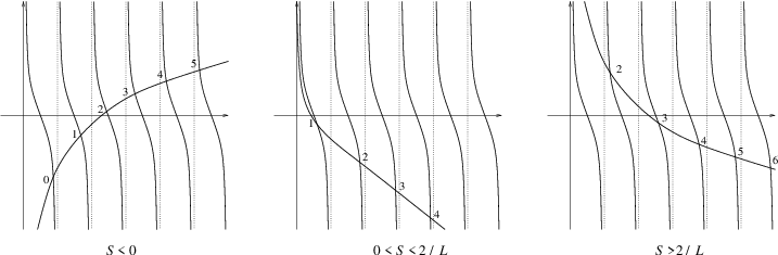
For each such we have the plane wave
| (6.25) |
There may also be a non-oscillating mode spanned by exponential functions . The condition reads
from which we find that the allowed value of is
| (6.26) |

See Fig. 9 for the pattern of solutions to this equation. For , there is no solution other than for which the function is zero. At , there is one solution for which is a constant mode. For , the solution is at . For , there are two solutions, one at and another at . These two values of converge to rapidly as grows;
These additional modes can be written as
| (6.27) | |||
| (6.28) |
Note that at and at . For , these modes are localized near the two boundaries.
The modes are labeled by at any value of — for they are all oscillating modes while for the first two are exponential modes. These functions are normalized as
If we expand the field as
the Lagrangian reads as
| (6.29) |
where it is understood that and/or whenever it applies.
The boundary conditions of the fermions , are satisfied by and respectively, provided obeys the equation
| (6.30) |
There are solutions labelled by a half integer such that
The starting number depends on the value of (See Fig. 10):

For each such , we have the plane-waves
which are normalised as
On this subspace of wavenumber , the kinetic operator is expressed as
and it is diagonalized by
| (6.31) |
There may also be eigenmodes spanned by exponential functions — there is indeed such a mode for solving
| (6.32) |

There is no non-zero solution if , and there is a single non-zero solution when (see Fig. 11). It approaches rapidly as grows,
Thus, this exponential mode can be regarded as the replacement of the oscillating mode that is missing for . The modes are obtained by simply replacing by in , explicitly,
| (6.36) | |||||
In the limit , approaches zero but approaches a non-zero linear function. Thus, for any value of the modes are parametrized by positive half-integers . If we expand the field as
the Lagrangian is expressed as
| (6.37) |
where it is understood that if .
6.3 The Ground State
Let us next quantize the system. Looking at the Lagrangian, (6.19) and (6.23) in the Ramond sector, (6.29) and (6.37) in the NS sector, it is clear what to do.
The bosonic system is simply the sum of harmonic oscillators. For each mode we introduce creation and annihilation operators
| (6.38) |
where we need two sets, , since we have complex (two real) oscillators. The variables and their conjugate momenta can be written as
or equivalently, for ,
where (resp. ) in the Ramond sector (resp. NS sector). The Hamiltonian of the system is the standard one
| (6.39) |
For the fermion system, it is simply to require the anticommutation relations to the mode coefficients
| (6.40) |
where the indices are for . In the Ramond sector, we also have the non-oscillating modes, and , which obey
| (6.41) |
and anticommute with all others, and . The Hamiltonian is given by
| (6.42) |
with the addition of
| (6.43) |
in the Ramond sector. Here, we have chosen the standard operator ordering .
The ground state of the system is the state annihilated by all annihilation operators
| (6.44) |
In the Ramond sector, we need an additional condition — if , the ground state must be annihilated by while it must be annihilated by if :
| (6.45) |
The energy gap to the first excited state is . In the Ramond sector is understood as and thus the gap is . For , the gap vanishes. In this case, the exponential modes for the scalars have vanishing potential, see (6.19), and the ground state wavefunction is not normalizable in the directions. In addition, there is a two-fold degeneracy from the exponential mode from the fermion. In the NS sector, is non-negative for but is negative, , for . As approaches zero while is positive, turns negative (this occurs when provided ). In such a case, the potential for the exponential mode is unbounded below, see (6.29), and there is no ground state in the system. The appearance of the zero mode or unstable mode at special values of is extremely important and plays a crucial rôle later in this paper. For now, we focus on the cases where there is a unique normalizable ground state and study its energy and charge.
6.4 The Energy
Let us compute the energy and its density of the ground state.
6.4.1 Total Energy
R sector
The computation in the Ramond sector is extremely simple: For each non-zero mode, the positive energy from the boson and the negative energy from the fermion cancel out;
The ground state energy from the bosonic zero mode is . The ground state energy from the fermionic zero mode is if and if (see (6.45)), that is, for any case. They fail to cancel against each other, Thus, the gound state energy in the Ramond sector is
| (6.46) |
NS Sector
The energy of the ground state in the NS sector is less straightforward to compute, but it is possible to find the answer in the limit .
Let us first start with the case where the bosons have integer modes , and fermions have half-integer modes , . The ground state energy is
| (6.47) |
This is infinity minus infinity and we need an appropriate regularization to define the sum. We do this using the fact that the sum over
is finite. Namely, we evaluate the sum (6.47) as
Thus, in the limit we have
| (6.48) |
The validity of this regularization will be examined momentarily.
Let us move on to the case with non-zero . We are interested in the limit of large for a fixed , so that we may assume . We divide the total energy into two parts, the part coming from the oscillating or constant modes and the part coming from the exponential modes. The latter part is present for but is absent for . To find , we first compute the derivative and then integrate,
The sum is over , if while it omits and if . The equations determining and are in (6.24) and (6.30) respectively, from which it follows
where are terms that vanish as (in what follows such terms will not be mentioned). Thus we find
This is logarithmically divergent and we introduce a cut-off :
where , with or . Integrating, we find for
Here, arctangent is assumed to take values between and . Let us now determine . We recall that the spectrum of oscillating modes is continuous as approaches from below (the lowest mode converges to the zero mode). Thus we have . On the other hand, we loose two bosonic and one fermionic oscillating modes as is increased beyon . Since each mode comes with a pair (complex for boson and for fermion), we have
Using these we find
If , which actually means , we need to add the contribution from the exponential modes,
After the addition, the term in becomes just for any value of . In this way, we find that the total energy is
| (6.55) |
6.4.2 Energy Density
Let us next compute the vacuum energy density, defined as the vacuum expectation value
| (6.56) |
of the Hamiltonian density
R Sector
In the Ramond sector it is
Let us focus on the region near the left boundary , and take the limit. In this limit, the last term becomes
Thus, the density can be written in the limit as
| (6.57) |
If is strictly away from the boundary, , one may proceed the computation as follows:

| (6.58) | |||||
From the second to the third line, the contour is deformed as in Fig. 12 using the fact that is strictly positive. Note that there is a simple pole at only when is negative, which produces the additional term , which in turn is canceled against the contribution from the exponential mode.
We see that the density is localized near the boundary with widths . Let us compute the total of this localized energy by integrating the density after the limit . (This is different from integration before the limit, which simply reproduces the total energy given in (6.46).) Since the integration domain includes , we must go back to the expression (6.57) before the contour deformation of Fig. 12. Also, we need to cut off the momentum integral at :
At this stage we use
and also the fact that
decays exponentially as — as can be shown by deforming the contour as in (6.58). Then we find
| (6.59) |
The integral on the right hand side is defined to be zero for . For , it can be evaluated;
Thus the localized energy at is
| (6.60) |
Let us next compute the energy localized near the right boundary , where we use the coordinate . Namely, we take the limit of keeping finite. Since the wavenumbers are , we have equations and that allow us to write the energy density in the coordinate:
The limit can now be taken straightforwardly:
| (6.61) |
Proceeding as before, we find
| (6.62) |
and
| (6.63) | |||||
Note that
see (6.46). This means that the total energy comes purely from the energies localized at the two boundaries. This is consistent with the fact that the energy density vanishes in the bulk of the interval .
NS Sector
Let us next discuss the energy density of the ground state in the NS sector (6.2). Actually, we know what to expect: At the right boundary , the boundary condition is exactly the same as the Ramond boundary condition and thus we should obtain the same answer as . The NS condition at the left boundary is obtained from the Ramond condition at the right boundary , by , . Therfore we expect that for close to is obtained from at close to , by the replacement . To summarize, the expectation is
and
| (6.76) | |||||
The sum of the two is is nothing but the total energy (6.55) of the NS vacuum.
One can indeed verify the above expectations. We split the density into two parts, the part from the oscilating or constant modes, and the part from the exponential modes that are present only for . We first consider the contribution from the oscillating/constant modes. By definition we have
See Section 6.2.2 for the quantities that appears here. In particular, and are defined by the equations (6.24) and (6.30). Let us look at the behaviour near the left boundary , taking the limit for a finite . In this limit, the difference between neighboring wavenumbers disappears , and we have for a finite . Thus we have
where are terms that vanish in the limit. Let us now look near the right boundary : take the limit with kept finite. To do this, we write everything as a function of . Using the defining equation of and we find
In the limit the sum over the modes becomes an integral over where the difference of and disappears. Noting that for , we find
We next consider the contribution from the exponential modes, which are given by (6.27), (6.28) and (6.36). These functions behave as follows, in the limit for finite and finite ,
The contribution to the energy density is
The sum leads to the expected answer (6.4) in the limit .
6.5 The Charge
Let us compute the charge of the ground state. The charge density operator is defined by
| (6.109) |
and we want to compute the eigenvalue of the total charge
of the ground state and the vacuum expectation value of the density
R Sector
Using the mode expansion, we find that the density operator is expressed as
| (6.110) | |||||
in which we set and , and the total charge is
| (6.111) |
The ground state is annihilated by if and by if . Thus, it has charge
| (6.112) |
The charge density is
| (6.113) | |||||
Let us look at the neighborhood of the left boundary by taking the limit for a finite . In this limit we have
| (6.114) |
If is strictly away from the boundary , it is
| (6.115) |
We see that the charge is localized near the boundary with width . The total localized charge is
| (6.116) | |||||
Let us next look at the neighborhood of the right boundary . In the limit for a finite , we have
| (6.117) |
If is strictly away from the boundary , i.e. , it is
| (6.118) |
Again, the charge is localized near the boundary. The total is
| (6.119) | |||||
We note that the sum of the localized charges reproduces the total charge given by (6.112).
NS Sector
The charge density operator can be expanded in terms of the modes as in (6.110), from which it follows that
| (6.120) |
In particular, the vacuum has zero total charge,
| (6.121) |
The charge density of the ground state can be determined either directly or by employing the symmetry argument as in the computation of the energy density. In the latter method, we consider the transformation , that maps the Ramond boundary condition at to the NS boundary condition at . Note that it flips the sign of the charge density, . In either way we find
and
| (6.134) |
In Fig. 13, we plot the graph of the function (6.119)=(6.134) that shows the charge localized at the right boundary, for both Ramond and NS sectors.

6.6 Note On Supersymmetry
Let us comment on the supersymmetry of the states. The system in the Ramond sector has an supersymmetry which transforms the fields as
By Noether procedure we find the supercharges generating them;
| (6.135) |
where
The supercharges obey the supersymmetry relations with equivariant parameter ;
| (6.140) | |||
| (6.141) |
The operator on the right hand side of the first equation is the total charge operator (6.111) (not a supercharge).
We note that each term of and has an annihilation operator. This is obvious for the modes but is true also for the mode; see the property (6.45) of the ground state. Therefore, the ground state is supersymmetric, i.e., annihilated by both of the supercharges
The energy and the charge of the Ramond ground state is computed in (6.46) and (6.112); The energy is while the charge is . These are perfectly consistent with the supersymmetry algebra (6.140) and the fact that the state is supersymmetric. The ground state has positive energy but it does not mean that supersymmetry is broken in this matter sector.
6.7 The Case Of The Half-Space
Let us comment on the theory formulated on the half-space, say,
| (6.142) |
To be specific, we consider the boundary conditions which are the same as in the “right boundary ” of the finite interval. Namely we add the term (6.2) at the boundary and impose the associated boundary conditions (6.3) there:
As in the finite interval there are oscillating modes and exponential modes. Oscillating modes for the fields and , or are
| (6.143) |
for any positive . In addition, and may have exponential modes, proportional to
| (6.144) |
They are normalizable when is positive. Since they decay rapidly as , we shall call them decaying modes. They have a frequency and become zero modes when , that is, when . If is negative, the function grows exponentially and will not be considered.
Mode expansion and quantization is straightforward. It is simply to consider the limit of the finite interval theory — we only have to discard the modes that vanishes in that limit (such as the exponential mode in the Ramond sector of the theory, and a linear combination of the two exponential modes of the NS sector in the and theory). The fields are expanded as
| (6.145) | |||||
| (6.146) | |||||
where and are the eigen modes of the kinetic operator defined by
The mode operators obey the (anti-)commutation relations
so that the fields obey the canonical (anti-)commutation relations
Note that we need the decaying mode (in the case ) for this to work.
The ground state is the state annihilated by all the annihilation operators and, in the case ,
| (6.157) |
This is because the decaying mode contributes to the total Hamiltonian by
which has value (resp. ) for the state annihilated by (resp. ). The energy gap to the first excited state is for and is for from the decaying modes of and . It vanishes at where the decaying modes become zero modes. In particular, the ground states are two-fold degenerate and non-normalizable.
We can easily obtain the energy (density) and the charge (density) of the vacuum — we simply use the result of the limit of the finite interval theory:
| (6.158) | |||||
| (6.159) | |||||
The formula (6.158) agrees with the result obtained in [67]. Alternatively, one can find these results independently of the finite interval computation, directly from the above mode expansions. Then, we can learn about the finite interval theory. In particular, we can reproduce all of the results on the energy (density) and charge (density) at least for the case is very large.
6.8 Cases With Several Matters
Let us record the results for the case where we have matter fields with charges . We just have to sum the results for the single field cases with , .
If the theory is formulated on the half space (6.142), the energy and the charge are localized near the boundary, and the totals are
| (6.160) | |||||
| (6.161) |
where “arctan” is assumed to take values between and .
If formulated on the interval, the energy and the charge are localized near the two boundaries. The ones at the right boundary, , are the same as on the half space, (6.160) and (6.161), for both NS and Ramond sectors. The ones at the left boundary, , depend on the sector. In the NS sector, the energy is the same while the charge is opposite, in comparison to (6.160) and (6.161). In the Ramond sector, the energy and the charge are opposite to (6.160) and (6.161) except the last terms involving the ’s. The total energy and charge are the sum of those localized ones:
| (6.162) | |||
| (6.163) |
Assuming the Calabi-Yau condition
the above formulae simplify, in particular
| (6.164) | |||
| (6.165) |
6.9 Gauge Dynamics
So far, we have set all the fields in the gauge multiplet zero, except the constant mode of the scalar component . If we want to obtain the effective potential for we need to integrate out the gauge field and the auxiliary field.
Let us consider the system on the interval with charges and on the left and the right boundaries respectively. The Lagrangian is given by
| (6.166) |
where is the matter sector Lagrangian — in the case of a single chiral multiplet with charge , it is the sum of the bulk part (6.1) and the boundary parts (6.2), (6.4). Integrating out the auxiliary field simply produces the D-term potential
When we quantize a gauge theory in operator formalism, it is best to switch to the canonical formulation. The action in the canonical formulation is given by (see e.g. [68])
| (6.167) | |||||
where is the charge density
| (6.168) |
and is the matter action
| (6.169) | |||||
It is easy to see that we get back the system with the Lagrangian (6.166) after integrating out , , . On the other hand, in the Hamiltonian formulation, they play the role of conjugate momenta for , and . ( are conjugate momenta for ). is a non-dynamical variable and imposes the Gauss law constraints.
We choose the boundary condition such that is allowed to vary at the boundary. The Gauss law constraints are then
| (6.170) | |||
| (6.171) | |||
| (6.172) |
They can be solved by
which is consistent if and only if the following condition is satisfied:
| (6.173) |
For a given pair of Chan-Paton charges, this is the condition on the state of the matter system: the charge of that state must agree with the difference of the Chan-Paton charges at the left and the right boundaries.
The Hamiltonian density of the total system, with the gauge condition , is given by
| (6.174) | |||||
where is the Hamiltonian density of the matter sector. The task is to find the ground state of the Hamiltonian and its energy. This is a hard problem. An exception is the case of a Dirac fermion with (massless Schwinger model) where the diagonalization can be done exactly. For the massive model, there are various approximation methods to treat this problem depending on the range of parameters, such as the relation of the gauge coupling constant and the mass of the matter fields. See for example [59]. Although this is a very interesting problem in its own right, we do not develop a thorough study in the present paper.
Instead, we take just one approximation method, which leads to the following answer for the energy density of the ground state:
| (6.175) |
In the above expression, stands for the expectation value with respect to the ground state of the matter sector, . Note that is the charge density which we have computed in Section 6.5. Also, in (6.175) is the energy density of the ground state in the matter sector, which was obtained in Sections 6.4.2 and 6.7.
Let us describe the origin of (6.175) and estimate the error. The exact answer would be obtained by integrating out the matter fields as well as the fields and , in a fixed background of . One way to perform this is to first integrate out the matter fields for a fixed general profile for and , and then integrate out the latter. At the first step, we may treat the coupling perturbatively and keep only the first order terms, that is, repace it with . This is the approximation that leads to (6.175). The discarded part starts with terms of the form
where is the energy gap between the ground state and the first excited state. The rest are of higher order in and . These errrors shift the gauge coupling as
As long as the shift is small compared to , we may say that (6.175) is a valid approximation, with an error given by power series in . Recall that the energy gap is of the order of the real part of , , provided the imaginary part is positive, , in the NS sector, and for any case in the Ramond sector. In such a case, the condition for the validity of (6.175) is
| (6.176) |
This is in addition to the condition which is already assumed in the bulk theory. In Section 7.4, we will obtain the same condition from a different perspective.
The gap in the matter sector comes from the exponential modes (the deacying modes) localized near the boundary. Recall that they become the zero modes or unstable modes when vanishes. In such a case, the whole idea of the effective action for the vector multiplet breaks down. We must treat those modes on the same footing as the vector multiplet fields. For example, we may integrate out the oscillating modes only, leaving the decaying modes dynamical. Then (6.175) is a Hamiltonian density operator that involves the decaying modes and the fields. Note that we no longer have an unstable potential for the decaying modes in such a treatment. Although this problem is important and interesting on its own right, we do not attempt to solve it here.
Thus, let us assume (6.176). Even in such a case, one may still wonder if the expression (6.175) makes sense, since as well as diverges at the boundary and their squares may be dangerous. To examine this and also to find how the answer bahaves as a function of , let us compute the total of the electrostatic and D-term energies. This is enough to see whether there is a problem locally, since these two terms are positive semi-definite.
Let us first compute it in the Ramond sector. The mode expansion leads to the expression
Using this we find that the energy from the D-term potential is
| (6.177) | |||||
where it is understood that so that . Also, using the expression (6.113) for , we find that the electrostatic energy is
| (6.178) | |||||
Despite its appearance, this is continuous at , with
To obtain the last expression, we have used the formula
The behaviour at large is
Here is the charge localized near the left boundary (6.116). The result is regular everywhere away from the locus which we excluded by (6.176). The quantity inside the parenthesis in the extensive part should be defined as the series that appears in the first expressions (6.177), (6.178) — an error of order there would affect the non-extensive part. Note that it is finite as the cut-off is removed, since the FI parameter depends on it as . The sum of the D-term and electrostatic energies, , is thus
| (6.179) |
where
Let us next write down the result for the NS sector. We have to treat the three cases, , and , separately. The main point is that it is continuous at , with
with
To obtain this, we used the formula
The behaviour at large for the general value of is
where is the localized charge given now by (6.134). The result is regular everywhere away from the excluded locus . The sum of them is
| (6.180) |
where is as in the Ramond sector, with from (6.134).
The main conclusion of these computations is that, in both R and NS sectors, the D-term and electrostatic energy of the ground state behaves as
| (6.181) |
is a function of , independent of , which is regular everywhere except . This also holds in the theory with multiple fields of various charges.
This concludes that there is no danger from taking the square of a quantity that diverges at the boundary. Furthermore, we see that the dominant part of the vacuum energy, for large with a fixed , is the localized energy from the matter sector which grows linearly with . Compare (6.181) with the expressions obtained in earlier subsections, for example (6.160).
An Anomaly
Although it is not directly relevant for the main discussion of this paper, we would like to comment on an anomaly in the Ramond sector that comes from the Gauss law constraint. We consider a gauge theory with matter fields of charges , which we assume integers with q.c.d..
The Gauss law implies that the total charge of the state in the matter sector must match the difference of the charges and which we place on the two boundaries, (6.173). We usually take both and to be integers, and hecne must be an integer. The total charge of a state in the matter sector is an integer plus the charge of the ground state. In the NS sector, we found that the charge of the ground state vanishes, see (6.163). Thus, the charges of all states are integers. In the Ramond sector, on the other hand, the charge of the ground state is obtained in (6.163), from which we conclude that the charges of all states are modulo integers. Thus, we find a conflict with the Gauss law when
| (6.182) |
In the context of linear sigma models, this is precisely the case when the corresponding toric variety is not a spin manifold. In an open string Ramond sector of the non-linear sigma model, we need to have a spin structure of the target space in order to quantize the fermionic zero modes. The above anomaly is understood as the Coulomb branch counterpart of this. There is of course no problem when the Calabi-Yau condition is assumed, .
6.10 Mass From Superpotential
We now turn to a different system: the LG model of two variables with superpotential
where is taken to be real positive. We also consider a D-brane correponding to the matrix factorization
We may regard this as a part of the matter sector of a gauge theory in which and have charges and . If we write the matrix as , then and have gauge charges and respectively. In this section we study the property of the ground state of the open string whose both ends have the brane . In particular, we are interested in the energy and charge density of the ground state, especially in the limit where the length of the string is taken to be very large.
Before doing any computation, we already know quite a lot about the ground state. First of all, there is just one chiral ring element proportional to the identity
| (6.183) |
Thus, by the spectral flow, we know that there is a unique supersymmetric ground state. In particular the ground state energy is zero
At this point we recall that any quantum field theory formulated on a compact space, such as the interval we are considering, behaves like quantum mechanics. In particular, any symmetry present in the system cannot be spontaneously broken by the ground state . In the present open string system, there are two symmeties in sight. One is the charge symmetry (under which has charge ). The other is the parity symmetry that swaps the left and the right boundaries. That the symmetry is unbroken means that the ground state has charge zero:
That the parity symmetry is unbroken means that the energy and charge density of the ground state is symmetric under :
Finally, one more important fact is that the bulk theory has a mass gap. This in particular means that any local observable approaches the value of the bulk vacuum when it is far enough from the boundary, that is, when . In particular we expect
in that regime. Namely and might have a non-trivial profile but that is confined in a region of width near the two boundaries. Moreover, the parity symmetry as well as tell us that the total energy and the charge accumulated near each of the boundaries vanish. Thus, for a long distance observer, it looks as if the energy and the charge density identically vanishes without any delta function support at the boundaries. In what follows, we confirm this expectation by an explicit computation.
The system (6.1) we considered in the bulk part of this section does not have the parity symmetry . To be precise, there would be a parity symmetry only when it is combined with a sign flip of of and a complex conjugation of and . Thus, the energy and charge densities are not symmetric under the parity but only so when the appropriate operation is applied.
Explcit quantization of a related system had been done in [52] and later also in [35]. These works studied the Dirichlet boundary condition in the same bulk theory. That brane can be obtained from the above matrix factorization by replacing , by , and taking the limit .
6.10.1 The Ground State
The Lagrangian of the open string system reads as
| (6.184) | |||||
Note that the boundary fermions have the opposite orientation of time. In particular, they have the “wrong” sign kinetic term and obey the non-standard hermiticity relation
with respect to the standard orientation of time.
We take the standard supersymmetric Neumann condition for the bulk fields:
| (6.185) |
Note that this does not agree with the one coming from the variational principle. For example, the condition on from the variational principle would be
but we take the Neumann condition at both boundaries. However, we will find no problem in quantization. In fact, the boundary conditions from the variational principle will show up in an interesting way.
This system has symmetry: has charge and has charge . There is also a parity symmetry
that commutes with the symmetry.
The action is quadratic in all fields and the quantization is straightforward provided we find a clever choice of variables. The bosonic part is a decoupled sum of four copies (two from and two from ) of the real scalar field with Lagrangian
where and
| (6.186) |
The fermionic system decomposes into two sectors. Let us take the linear combination where is the spinor index and then introduce
for , . The Lagrangian can be written as
where and
Here is the evaluation map, and .
The kinetic operators , are hermitian operators in the space of functions defined by (6.185): Neumann for and Dirichlet for . Thus, they have eigenvectors with real eingenvalues. Let us diagonalize these operators. To this end, we introduce projection operators onto Neumann and Dirichlet functions
where , and . They obey the following relations
| (6.195) | |||
| (6.196) | |||
| (6.197) |
Using the first two, we find
Thus, if obeys the boundary condition
| (6.198) |
is simply represented by . At this point, we notice that this boundary condition for is precisely the same as the boundary condition for the boson in the system considered earlier: the NS condition (6.2) for with . In particular, for a plane wave the allowed wavenumbers are determined by the equation (6.24) with . As before we denote the solutions by , , which approach as .
For the fermion , the equations both lead to
This can be obtained by eliminating and from the three equations and using (6.195) (6.196) and (6.197). Again we find the standard eingenvalue problem provided obeys the boundary condition (6.198). In particular, we have plane wave solutions with eigenvalue , where solves (6.24) with .
Normalized modes are given as follows: For bosons, we have
| (6.199) |
and for fermions
where
Expanding the fields as
the Lagrangian can be written as
The Hamiltonian is
| (6.208) |
where , , , are the creation and annihilation operators obeying the standard (anti-)commutation relations. There is a unique ground state characterized by
Let us discuss the energy and its density of the ground state . The bosonic and fermionic contributions to the energy cancel at each level: . Therefore the total energy of the ground state vanishes:
| (6.209) |
This is of course a consequence of supersymmetry. To find the energy density, let us introduce the notation
Then, the energy density operator can be written as
| (6.210) | |||||
The energy density of the ground state is
| (6.211) | |||||
It is indeed symmetric under , as one can see by using .
Let us next discuss the charge of the ground state. The charge density operator is defined by
The total charge as well as its density of the ground state vanish
| (6.212) | |||
| (6.213) |
This matches with the expectation.
6.10.2 Limit
Let us look at the energy density in the limit where is very large compared to . We first look at the region close to the left boundary , that is, . The formula (6.211) can be rewritten as
In the limit the sum over turns into integral over the momentum . If is close to but strictly away from , the contour of the integral can be deformed and we have
| (6.214) |
We see that it decays exponentially as or faster. This is of course a consequence of the mass gap of the bulk theory. By the symmetry , we find the same behaviour near the right boundary . Namely, the energy density is non-trivial only in the region of width near the two boundaries. Since the total energy vanishes (6.209), we learn that the energies localized near the left and the right boundaries vanish indivisually. Indeed that can be confirmed by a direct computation:
The last term comes from the delta function at — the one at of course does not contribute. The two lines cancel out and we have .
6.10.3 Limit
For completeness, let us consider the opposite regime, . In the limit , the momenta approach the standard value
In particular, the mode approaches the constant mode while the modes approach the standard plane wave modes , for . To be more precise, using the defining equation (6.24), we find that diverges as
but it is still true that the mode approches a constant, and , as long as is in the interval . Let us look at the ground state in this zero mode sector.
In the limit , the fermionic zero mode becomes
Thus, we can write , , , Since the ground state is annihilated by , it is annihilated by
It follows that the zero mode ground state is of the form
where is the state annihilated by as well as the bosonic annihilation operators. (Note the normalization .) Recalling the definition of , and using the matrix representation of , , etc,
we find that the ground state is given by
| (6.229) |
Here, is the state of the bulk zero mode sector that is annihilated by as well as the bosonic annihilation operators. As a wave function of , it is proportional to . The state (6.229) is indeed annihilated by the zero mode supercharge
Note the normalization . It indeed corresponds to (6.183):
in the holomorphic truncation.
7 The Grade Restriction Rule
We now discuss the first main quantum effect of the linear sigma model with boundary. The goal of the paper is to construct parallel families of boundary interactions over the bulk of the Kähler moduli space, including in particular the boundaries between different phases. At each phase boundary, at least one subgroup of the gauge group is unbroken, and the corresponding Coulomb branch has a bounded bulk potential which vanishes exactly at the singular point. The focus of study will be the behaviour of boundary interactions and boundary conditions on that Coulomb branch. This leads us to the grade restriction rule (or the band restriction rule), which classifies the Chan-Paton representation of the gauge group for the D-brane that can be transported across the phase boundary. This is the main result of this paper.
7.1 A-branes In LG-Models
The theory on the Coulomb branch is described in terms of the twisted chiral superfield and has a superpotential which is classically . Note that B-type boundary conditions on twisted chiral superfields are like A-type boundary conditions on chiral superfields. To pave the way to discuss the boundary condition of bulk fields on the Coulomb branch, we briefly digress to reexamine the general requirement for A-branes in Landau-Ginzburg models. For simplicity, we consider the LG model of chiral superfields spanning a flat Euclidean space , with some polynomial superpotential .
It was argued in [69, 9] that an A-brane in a LG model is a Lagrangian submanifold whose image in the -plane must be parallel to the real line, or equivalently
| (7.1) |
on the brane. It is definitely true that (7.1) must be satisfied as long as we use the standard bulk action without a boundary term and impose the standard D-brane boundary condition. By the standard D-brane boundary condition we mean Dirichlet on normal and Neumann on tangent coordinates along with the condition on fermions that follows from supersymmetry. However, the requirement (7.1) is relaxed if we modify the action by a suitable boundary interaction which leads to a non-standard boundary condition.
Let us first examine the supersymmetry of the boundary conditions themselves, which does not depend on the detail of the action. It is convenient to use the real components of the chiral superfields, (), which are related to the complex ones as , , . We also introduce
in additon to . The variation of these component fields reads
| (7.2) |
where is the complex structure (multiplication by written in real coordinate): and all other entries are zero. is the parameter of the supersymmetry while is the extension to . We find an invariant set of boundary conditions of the form11 1 There are more general boundary conditions which eventually lead to coisotropic branes [70]. However, they require at least complex dimension two, . Since we are primarily interested in the Coulomb branch, especially for gauge theories, we shall focus on the conditions of the type (7.3).
| (7.3) |
for some submanifold of . This is consistent and complete when and have no overlap (except the origin ) and span the whole of ,
Such an is called a totally real submanifold of . It must be middle dimensional, . To summarize, we have an invariant set of boundary conditions (7.3) for each totally real submanifold of .
Let us next examine the invariance of the action. We first take the standard bulk action without a boundary term. Its variation is
| (7.4) | |||||
Vanishing of the term requires that and must be orthogonal to each other,
For a totally real submanifold , this is nothing but the condition that it is a Lagrangian submanifold with respect to the symplectic structure . Once that is satisfied, the only remaining condition is that . Since the vectors and are tangent to , this means that is locally constant on . This is how the requirement (7.1) arises. It is easy to see that the boundary condition (7.3) is consistent with the variational equation from the standard action: Since the action has no boundary term, the variational equation requires that must be normal to the brane. Since is normal to we find that and must be independently normal to . If we use the bulk equation for the auxiliary field
| (7.5) |
the condition that is normal to is automatically satisfied provided is constant on . This is the basic story of [9].
The standard bulk action can be modified by a boundary term so that it is invariant without use of any boundary condition. In fact one can write down a manifestly invariant action as follows:
| (7.6) | |||||
Here we used the Kähler potential . If we use this action, obviously, no requirement should arise from the invariance. This time, however, a condition comes from the consistency of the boundary condition (7.3) and the variational equation from (7.6), which reads
From the fermion terms, we find again the condition that must be orthogonal to , that is, must be a Lagrangian submanifold. If we use the bulk equation for the auxiliary field (7.5), the -terms combine to give , which is again satisfied under . This leaves us with the equation . This is not satisfied for an arbitrary Lagrangian submanifold — it has to be a Lagrangian plane that goes through the origin , that is, a linear Lagrangian subspace of . Note that we have the modified Neumann condition
| (7.7) |
in the direction tangent to the brane.
We have found that the manifestly invariant action (7.6) admits only a very spacial class of D-branes — linear Lagrangian subspaces. In fact, one can modify the action by adding a boundary term that is by itself invariant. For example, we may add a boundary D-term
| (7.8) | |||||
for some function of . We see that this changes the boundary term of (7.6) as
which corresponds to a Hamiltonian deformation of the brane . Thus, D-term deformations on the boundary generate Hamiltonian deformations of the brane. If is linear in ’s then this simply corrsponds to a parallel displacement of . If is quadratic it corresponds to a symplectic rotation of . For a more general function, we obtain a more general Lagrangian submanifold. This is one way to obtain more general D-branes than just linear Lagrangian subspaces. Alternatively, we may simply take
| (7.9) |
It is not automatically invariant but the invariance requires only the Lagrangian condition . The variational equation is then solved again by (7.3) that includes the modified Neumann condition (7.7). Thus, we find an A-brane for any Langrangian submanifold . The imaginary part of does not have to be a constatnt on .
In the new formulation, with the action (7.6) or (7.9), the system has a potential energy at the boundary
| (7.10) |
The imaginary part of a holomorphic function is unbounded below and above on . Thus, depending on the asymptotic direction of the brane , the boundary potential can be unbounded below. To avoid any problem associated with it, we propose to require that must be bounded below on the brane . Necessity of such a constraint is not so obvious since there is also a bulk potential An exception is the case where is linear, which is the main focus of the present section: the bulk potential is constant whereas the boundary potential is linear. In this case, it is absolutely necessary to require that is bounded below at every infinity of the brane . When is quadratic or higher, it is less clear whether we need the constraint. However, as we shall see below, it is preferable to keep this requirement also in the general case.
If we loose the requirement (7.1), the set of allowed D-branes is considerably expanded. However, we may identify the branes that are related by boundary D-term deformations. We have seen that a Hamiltonian deformation of the brane corresponds to the boundary D-term of the form (7.8). Here we must be careful — (7.8) can be regarded as a deformation only when its effect is small at infinity in the field space. In the absence of a superpotential, we need to assume that the function approaches a constant at infinity or a linear function at most. For example, a quadratic function corresponds to a rotation of the brane and cannot be regarded as a “deformation” since it results in an indefinitely large move at infinity. The parallel displacement, corresponding to a linear , is the marginal case where one may or may not regard it as a deformation. In the presence of bulk and boundary potentials, a higher power of is allowed as long as the effect is small relative to the effect of the potentials. In fact, as long as the potentials grow fast enough along the brane , the wavefunction in that infinity direction is damped exponentially, so that the Hamiltonian deformation for almost any function can be safely regarded as a boundary D-term deformation.
An important invariant under the boundary D-term deformation is the overlap of the boundary state with a R-R ground state , known as the generalized central charge. (Here we assume that the polynomial is quadratic or higher so that there are supersymmetric ground states as many as .) It is realized as the path integral on a semi-infinite cigar and is represented as the integral:
| (7.11) |
Here is the circumferemce of the boundary circle of the cigar and is the differential form on of middle degree that corresponds to the ground state . To be precise, the form realizes the ground state of the supersymmetric quantum mechanics obtained by compactification on the circle of circumference . See [52] for details. It is normalizable and has the asymptotic behaviour . Although it indeed decays exponentially at infinity, the factor coming from the boundary potential (7.10) can be dangerous if extends to the direction with . Thus, Hamiltonian deformations of across that dangerous hypersurface cannot be regarded as boundary D-term deformations. Therefore, we should better avoid that hypersurface. Given the freedom to use boundary D-term deformation, we may even require that grows at every asymptotic direction of . In that case the integral (7.11) can be recast into an integral of a holomorphic differential [52].
This picture of A-branes in LG models is consistent with all known results based on (7.1) and also on other methods. It actually explains some of the puzzles in the old picture. For example, in [9] only branes with constant and were considered, and those with were completely ignored. In the new picture, those branes with and those with are connected via D-term deformations through the region with large positive . There is a one to one correspondence between the D-isomorphism classes in such two sets of branes. For illustration, let us consider the LG model for the minimal model . If we require , a brane is a union of two rays in the directions , . However, only rays in the directions , were considered in [9]. In the new picture, each ray can be in any direction bewteen and so that is bounded below at infinity. Fig. 14 shows the case .

The dashed line is an example of a brane taken in [9] while the centipede line satisfies but was ignored. In the new picture any brane is allowed as long as it has asymptotic region with positive . The solid line is such an example and it indeed connects the dashed line and the centipede line. For the branes preserving the opposite supercharge (or for the branes preserving the same supercharge but on the left boundary), the boundary potential has the opposite sign, , and thus the requirement is that is bounded above on . Then, the rays must be between and . This alternation pattern has been observed in the geometrical picture of D-branes in the gauged WZW model (Kazama-Suzuki model) that realizes the minimal model [38].
7.2 Asymptotic Condition In The Coulomb Branch
We now come back to the study of boundary linear sigma models. Our focus will be the boundary condition on the Coulomb branch. As discussed in the previous section, we need to specify a Lagrangian submanifold on which the boundary potential is bounded below. We first consider a model with gauge group and assume the Calabi-Yau condition
In the region with large , it is appropriate to integrate out the charged matter fields. This yields corrections to the potential and kinetic terms and also produces higher derivative terms. Corrections to the kinetic term and higher derivative terms are written as power series in and and are negligible in the low energy limit in the region . Therefore, we can use the classical kinetic term (5.2) in that regime. Since it is written in the manifestly supersymmetric form with quadratic Kähler potential, as discussed in the previous section, the Lagrangian must be a linear Lagrangian subspace. Namely, it must be asymptotically a straight line in the Coulomb branch. Of course the correction will be large in the region , and there is no reason for to be straight there. Thus, the Lagrangian is a bent line, coming in toward the origin from one asymptotic direction and going out to infinity in another direction. In order for the brane to be coupled to the Higgs branch theory, should better go through the region .
The correction to the potential can be non-zero even in the asymptotic region. In the bulk, the twisted superpotential is corrected simply by the shift of the FI-theta parameter,
The ambiguity of the imaginary part is fixed by the boundary charge. Quantum corrections to the boundary potential and the boundary charge were analyzed in Section 6. For the Wilson line brane with charge , the effective boundary potential is
and the effective charge is
| (7.13) |
The potential can indeed be written as with where . (In comparison with (7.10), the factor of is just a convention and the sign is the difference between chiral and twisted chiral superpotentials.)
Note that there is a discontinuity in the effective charge and singularity in the potential at , that is, on the imaginary line. This is due to the appearance of zero modes from the charged matter sector: The decaying modes localized at the boundary become zero modes exactly at for positively charged fields and at for negatively charged fields. In those directions, no matter how large is, the matter fields are not really decoupled from the low energy dynamics. The effective description purely in terms of breaks down at . In this sense we shall sometimes call the imaginary line a singular line.
The asymptotic lines for must be such that the boundary potential () is bounded below. Let us depict the region of positive boundary potential, for various values of and a fixed . The behaviour depends very much on the relation of and the charge shift ,
| (7.14) |
We consider three cases separately.


The boundary potential is positive in the shaded regions. If is larger than or smaller than , the positive potential region rotates roughly by degrees as is changed from to . Not a single Lagrangian can stay inside the region for all values of . On the other hand, if , the region does not rotate. In particular, the real line is always inside.
As discussed in the previous section, we can deform the brane as long as they stay inside the admissible region — that would be a boundary D-term deformation. If we use this freedom we notice that some of the configurations should be regarded as trivial. For example, we can consider deformations as shown in Figure 18.

When the two rays are deformed to coincide, brane-antibrane annihilation takes place. Alternatively, the brane may be detached from the center of the Coulomb branch. Then, it is decoupled from the Higgs branch theory and will eventually disappear to infinity. The existence of such deformations means that the starting configuration (left) should be regarded as trivial. This does not apply if the two rays of are on the opposite side of the singular line at . In order to move the two rays until they coincide, either one or both of them must hit the singular line. Also, even if the brane is detached from the origin, it will still intersect with the singular line and continue to be coupled to the matter sector.
7.3 Rules Of D-Brane Transport
We now describe rules of D-brane transport. We first consider models with gauge group and next the cases of higher rank gauge groups.
7.3.1 Gauge Group —The Grade Restriction
We are interested in transporting branes along a path that goes from the large volume phase to the small volume phase , or in the opposite direction. The path should better avoid the singular points at and .

Thus, it must go through the windows between the singular points. For simplicity, we consider paths that goes just once through one of the windows, as shown in Figure 19. (The Figure is for the case where is odd. For even , the windows are at , ). More complicated paths are just some combinations of such simple paths. We claim
The Grade Restriction Rule:
The Wilson line brane can be transported smoothly between
the two phases if and only if the inequality
| (7.15) |
holds in the window. The same can be said on a complex of Wilson line branes or a matrix factorization of the superpotential: each must obey the inequality (7.15) in the window in order for the brane to be transported smoothly.
For a given choice of window, this rule selects consequtive integers as the allowed set of boundary charges . For example, in a theory with , the allowed set is if the window is at . If we change the window to , the set changes to . Below, we provide a derivation of this rule.
Suppose the inequality (7.15) is not satisfied on the window. To be concerete, suppose that is too large for that. As we move along the path, say from to , the region of positive boundary potential rotates counter-clockwise as in Figure 15. The rays of must be rotated so that they are always inside that region. We depict an example of such a rotation in Figure 20.

The starting configuration (left) is chosen so that the two rays are on the opposite side of the singular line . As we have discussed above, this is required for the brane to be non-trivial. At some moment before we go through the window, the ray that was on the right of the singular line must overlap with the singular line on (second from left). At that moment, something non-trivial must happen to the brane. If nothing had happened, then after that we would have a configuration where both of the rays are on the left of the singular line (center). But that configuration is trivial as the brane would annihilate by admissible deformations. This is in contradiction to the fact that the starting configuration was non-trivial. Somthing non-trivial must also happen when the other ray overlaps with the singular line on (second from right). At this stage, we cannot exactly tell what really happens except that it has to do with the zero modes from the matter sector. Later in this paper, we will discuss this point from a different perspective.
Let us now consider the case where the inequality (7.15) is satisfied. If the path is a straight line at a constant obeying (7.15), then there is no need to move as the real line
| (7.16) |
is always inside the admissible region. If the path is curved as in Figure 19, then it may happen that the inequality is not satisfied along a part of the path. Then, we may need to deform away from the real line. However, as long as the inequality is satisfied on the window at , the admissible region is always on both sides of the singular line , and the two rays do not have to overlap with the line, never at any point of the path. Thus, the brane can be continuously deformed from one phase to another.
To summarize, we can consider branes for arbitrary boundary charges . They are non-trivial as long as the two rays of are on opposite sides of the singular line . However, only those obeying the grade restriction rule can be continuously transported between the two phases through the window. For a component of a brane which does not satisfy the grade restriction rule, the asymptotic condition on the Coulomb branch must overlap with the singular line along the way, and something non-trivial is expected to happen. This is the meaning of the grade restriction rule.
7.3.2 Higher Rank Gauge Group — The Band Restriction
We now consider the model with higher rank gauge group (). We are interested in transporting branes along a path that goes from one phase to another in the multi-dimensional Kähler moduli space . Here we focus on paths that go from one phase to an adjacent phase through the phase boundary in the asymptotic region, that is, the region with large values of FI parameters. Any two phases can be connected by a combination of such paths.
In the asymptotic region, there is exactly one subgroup of the gauge group that can be unbroken at the phase boundary. The remaining gauge group is completely Higgsed and can be ignored. Repeating what we have done before for the unbroken subgroup, we find a rule of D-brane transport. Let us arrange the basis of the Lie algebra of so that the first factor is the unbroken . Then, the coordinate is transverse to the phase boundary. The singular locus is asymptotically at and where
| (7.17) |
We fix one of the windows at and consider a path that goes though it. We have
The Band Restriction Rule:
The Wilson line brane
can be transported smoothly across the phase boundary
if and only if the inequality
| (7.18) |
holds in the window. The same can be said for a complex of Wilson line branes or a matrix factorization of the superpotential: each must obey the inequality (7.18) in the window.
There is no condition on . For a choice of window, this selects a band of width in the lattice of charge vectors. For example, let us consider the two parameter model (Example (C) in Section 4.4), and look at the boundary between Phase I and Phase IV. The unbroken subgroup is the original , with the number . If we choose the window at , , then the band is as shown in Figure 21 (left).

The Figure also shows a sample of bands at other phase boundaries; the I-II or III-IV boundary (middle) and the II-III boundary (right).
7.4 The Nature Of The Rule
The above derivation of the grade/band restriction rule is certainly concerned with the transport of D-branes in a linear sigma model with finite gauge coupling which is formulated on a worldsheet of finite (spatial) volume.
In fact, the effective boundary potential () as well as the effective boundary charge (7.13) ceases to be valid if we take the infinite coupling or infinite volume limit. The validity of a perturbative treatment of the gauge interaction that leads to these expressions had been analyzed in Section 6.9. Here we would like to discuss it from a different perspective. As before, we consider the strip of width . There is a bulk contribution to the total energy
| (7.19) |
The second term is the electrostatic energy: is the charge at the (right) boundary that determines the value of the electric field via the Gauss law. The boundary charge can be changed if we choose a different state from the matter sector. Such a change may reduce the electrostatic energy , but it may increase the energy of the matter sector at the same time. The effective potential and charge are obtained by finding the configuration that minimizes the total energy. The results () and (7.13) are obtained by ignoring the contribution of in the minimization problem. That is valid when the excitation energy in the matter sector is much larger than the possible change in by the change of boundary charge. The separation of the energy levels is of order for oscillating modes and for decaying modes. Thus, the region of validity is
| (7.20) |
This is indeed the same as the condition (6.176) we obtained earlier. In the opposite regime, , while is still much larger than the gauge coupling , the electrostatic bulk energy is much more important than the boundary potential. Then, the state in the matter sector must be such that the boundary charge minimizes the electrostatic energy. Thus, “the singular line” of purely imaginary , which played the crucial rôle for the grade/band restriction rule, is actually a singular band of width . This band spreads over the entire -plane if we take the infinite volume limit or infinite gauge coupling limit , or any limit that sends to infinity.
The key question is what is the rule of D-brane transport in a theory formulated on a worldsheet of infinite volume, or in the conformal field theory to which the linear sigma model flows to in the infra-red limit. Does the grade restriction rule still hold? Is there some phase transition that is not visible at finite volume and finite gauge coupling?
A similar issue was discussed in the bulk theory [4] concerning the meaning of the Coulomb branch analysis to the phase transition in the infinite volume system. It was first noted that the existence of a phase transition depends on the particular path in the multi-parameter space of theories. Then the focus was concentrated on the paths inside conformal field theories for which we know the answer from mirror symmetry. It was argued that the finite volume and finite coupling theory is enough to find all possible singularities of the conformal field theories: if the singularity is purely due to the vanishing of the Coulomb branch potential ( above), then the potential only seems to grow in the infra-red limit if that was non-zero for finite and finite . The only possible problem in this argument was the conflict of the condition for the Coulomb branch analysis and the infra-red limit .
The situation is much more subtle in the boundary theory. It is certainly the case that the existence of a singularity depends on the particular path in the multi-parameter space of theories. The grade/band restriction rule is derived for the path in the space at fixed, finite values of and : there is no singularity in the transport of the brane if and only if any of the boundary charges of the brane is inside the grade/band restriction range (7.15) or (7.18). Does it tell something about transport of the corresponding conformally invariant brane in the corresponding family of conformal field theories? For branes with charges outside the grade/band restriction range, the answer is simple. We do not even have a family of boundary conformal field theories from such a family of linear sigma model branes. This is so as long as they are defined as the infra-red limit of boundary QFTs with finite and finite . The grade restriction rule is valid as long as is finite, no matter how large it is. There is a problem already at finite volume and finite coupling, and hence there is nothing to study.
Things are non-trivial for branes with charges inside the grade/band restriction range. First of all, we do have a family of boundary conformal field theories from such a linear sigma model brane. The question is then whether there is a singularity along the way. There is no compelling argument like the one for the bulk theory that shows the non-existence of a singularity. On the contrary, it is expected that there are singularities or more appropriately transition points. We know many examples of D-brane decays when the closed string background is dialed through walls of marginal stability: on one side of the wall the brane is stable and on the other side it decays to, say, two stable D-branes. From the worldsheet point of view, the point of marginal stability can be regarded as a transition point in the family of boundary conformal field theories. Thus, it is not that there is no singularity if the grade/band restriction rule is obeyed. But it is that a grade restricted brane provides a family of boundary conformal field theories. It provides us with a starting point to study stability and D-brane decay.
7.5 The Full Boundary Conditions
Let us explicitly write down the boundary conditions on the bulk fields. For the Wilson line brane in a gauge theory, the Lagrangian submanifold
is in the admissible region as long as is in the strip domain , . Thus, we take it as a part of the boundary condition of the vector multiplet fields. The boundary conditions on other component fields, (7.3), read and . Actually, we may take as an extra condition since its variation is proportional to that of . In this way, we find the following set of boundary conditions
| (7.21) |
Another set of conditions follows from the Gauss law constraint:
| (7.22) |
If we use (7.21), the conditions on the matter chiral multiplet fields (5.47) simplify to
| (7.23) |
These are the full set of boundary conditions on the bulk fields. These are invariant under the supersymmetry and are compatible with the variational equation.
At a point away from the strip domain, only one half of the line is in the admissible region. As we have discussed, the two asymptotic lines of must be on the opposite sides of the singular line . Thus, we take to be the one obtained from by rotating one of the asymptotic lines so that it is in the admissible region. This is possible as long as . In particular, for or , we can take to be very close to the real line . The other set of conditions (7.22) can still be imposed. For the matter sector, we need to use the original condition (5.47) for the part of away from .
Remarks
(i) The condition on the matter fields (7.23) is identical to the ultra-violet boundary condition (5.48). At this moment we do not know the significance of this observation. One possibility is that the ultra-violet theory can be used to study some of the properties of the grade restricted branes. Indeed, as we will see in later sections, the theory provides correct results for the space of chiral ring elements for any pair of grade restricted branes.
(ii) When there are bulk and boundary interactions from the superpotential and the tachyon profile , the variational equation is changed and the boundary conditions should be modified. However, we can still use the above boundary conditions as long as we treat these interactions as perturbations. Recall the remark on this approach given in Section 5.5. Here, we would like to comment on the treatment of the Gauss law. Suppose a brane consists of more than one Wilson lines with various different charges . The Gauss law constraint shows that the bulk fields obey different boundary conditions for different Chan-Paton components of the same brane. This may look strange at first sight but a moment of reflection reveals that there is nothing wrong, at least in perturbation theory. In the path-intergal formalism, we expand the path ordered exponential into a Dyson series. Each term of the series is a product of matrices of the form , , , etc, which are inserted at points of the worldsheet boundary. These points separate the boundary into segments — each segment corresponds to one of the Chan-Paton components. Then, it is simply that we impose different conditions on different parts of the worldsheet boundary. In the operator formalism, the situation is even clearer. The Chan-Paton space is already a part of the quantum Hilbert space — an open string wavefunction is a product of the bulk part and the Chan-Paton factor. It is simply that the bulk fields obey boundary conditions that depend on the Chan-Paton factor.
(iii) That one can take an extra condition is a special feature of the Lagrangian submanifold . In fact a similar property is possessed by the singular line
on which the decaying modes from the matter sector become zero modes. One can take an extra condition , since its variation is identical to that of (that is why the combination is supersymmetric). The invariant set of conditions including these is
| (7.24) |
This may be completed by another set of conditions:
| (7.25) |
In fact, (7.21) and (7.24) are the only possible invariant sets that include two independent equations of the form and where are real valued functions of and . We do not yet understand the significance of this observation.
8 Non-Compact Models
In this section, we achieve our main goal of the paper: using linear sigma models, we construct parallel families of D-branes over regions of the Kähler moduli space that encompass various different phases. The key result of the previous section, the grade (or band) restriction rule, plays the most important role in the construction. This section focuses on models without superpotential, whose low energy theories are non-linear sigma models on toric Calabi-Yau varieties, possibly with orbifold singularities.
In Section 8.1 we study how D-branes of the linear sigma model descend to the low energy theories deep inside the phases of the Kähler moduli space. We proceed in two steps: First, we determine the low energy boundary interaction of a given complex of Wilson line branes (5.20). Second, we take into account D-term deformations and brane-antibrane annihiliation, named D-isomorphisms in Section 3, which do not change the low energy behaviour of boundary interactions.
In Section 8.2, we apply the grade (or band) restriction rule and transport D-branes along paths that connect adjacent phases, achieving our main goal of the paper. As a consequence, this leads to one to one correspondences between D-isomorphism classes of D-branes at different phases. Mathematically, this results in equivalences of the derived categories of different toric varieties.
As an application, we obtain an honest understanding of D-brane monodromies associated to closed loops in Kähler moduli space, which we shall consider in Section 8.3. In Section 8.4, we demonstrate the power of construction in typical examples: the (local) flop transition and the McKay correspondence. In Section 8.5, we discuss families of D-branes over the central region of the moduli space where multiple phase boundaries meet. We find a simple construction which works under a certain condition.
8.1 Low Energy Boundary Conditions
We first study the low energy behaviour of D-branes of the linear sigma model, assuming that we are deep in some phase in the Kähler moduli space where the gauge group is broken either completely or to its discrete subgroup. At energies well below the gauge coupling , the theory reduces to the bottom of the scalar potential, the vacuum manifold , possibly with orbifold points. Thus, we are interested in how the linear sigma model branes descend to D-branes in the non-linear sigma model on .
The low energy limit is achieved by the limit , in which the vector multiplet loses the kinetic term in the bulk. The auxiliary field becomes a Lagrange multiplier field that imposes the D-term equation strictly. The components and become auxiliary fields and the effect of elimination is to set them equal to their classical values, see (4.12)-(4.14). We claim that, under appropriate boundary condition on the vector multiplet, this picture remains the same also in the presence of a boundary with the boundary interaction (5.5) or (5.2) that includes , and . For concreteness, we consider a gauge theory formulated on the left-half plane, , and put the Wilson line brane at the boundary.
We first note that and appear only in the boundary counter term for the gauge kinetic terms, see (5.2) and (5.2). As we have discussed in Section 7.1, the boundary condition for the gauge multiplet fields are chosen so that this counter term vanishes. Thus, and do not appear in the boundary interaction. In particular, the effect of integrating them out remains the same as in the bulk: impose the D-term equation as a constraint and set equal to the classical value (4.13). The part of the action that depends on is
For simplicity of notation, we consider only a single charge matter field. Completing the square and integrating out , we are left with
The effect is simply to set equal to the classical value of the bulk theory (4.12), except that we acquire the boundary term that involves . This looks problematic. For integration, we find
Again, we find the unwanted at the boundary. However, we notice that it has the opposite sign and exactly the same absolute value compared to the term from the -integration. Thus, they completely cancel out. This cancellation occurs precisely when both and are unconstrained at the boundary. And this is indeed the type of boundary conditions we impose, as we have discussed in Sections 7.2 and 7.5. Otherwise, we may need to keep an uncancelled in the low energy theory. Our choice of boundary conditions saves us from such a complication. The appearance of at the boundary from elimination of auxiliary fields was found earlier in [71] where the significance of such a term to supersymmetry is discussed.
To summarize, the effect of intergrating out and also remains the same as in the bulk: set them equal to their classical values (4.12), (4.14). Accordingly, the boundary interaction for the Wilson line brane is expressed as
where the term is the pull-back of the connection on the holomorphic line bundle over . This is nothing but the boundary interaction for the D-brane in the non-linear sigma model supporting the line bundle , see (2.7). Thus, we find that the Wilson line brane descends to the brane supporting the line bundle
Things are as simple as this also for more general branes, direct sums of Wilson line branes with interaction . The corresponding boundary interaction (5.12) directly descends to the boundary interaction (2.28) of a D-brane in the non-linear sigma model, associated with the vector bundle with connection and tachyon . The R-symmetry also descends straightforwardly. Thus, the graded D-brane directly descends to the graded D-brane . In other words, a complex of Wilson line branes,
with , becomes a complex of holomorphic vector bundles over the target space ,
| (8.1) |
where the component of R-degree is a direct sum of line bundles, .
In the above discussion, we have assumed that is smooth, but everything goes through in the presence of orbifold loci as well, provided we consider a part of the gauge charges as the data of the orbifold group action on the Chan-Paton factors rather than the data determining the vector bundle with connection. When can be realized as a global orbifold of a space , we may regard as an equivariant line bundle over . In general, the correct mathematical name for it is a line bundle over the quotient stack , but not a sheaf over the algebraic varity (see [72] and Section 9). In what follows, somewhat loosely we call such objects simply “line bundles or vector bundles over the toric variety ”.
Let us introduce some notation. We denote by the set of graded D-branes in the linear sigma model. We denote by the set of graded D-branes in the low energy theory with target space . The map of D-branes obtained above is denoted by
| (8.2) |
In the following, we shall indicate the degree component of a complex by underlining it, , when there is a room of confusion. Also, a complex consisting of a single vector bundle at R-degree will be denoted by . For the one at degree 0, we may simply denote it by when there is no room of confusion.
D-isomorphisms
Let us now apply the concepts that are introduced in Section 3 to D-branes in the low energy theory. Namely, we regard D-branes to be isomorphic in (or simply D-isomorphic) if they are related by a combination of D-term deformations and brane-antibrane annihilation. Isomorphic D-branes in flow to the same infra-red fixed point, although the converse is not true in general. The map (8.2) is therefore the operation of modding out D-branes of the linear sigma model by D-isomorphism relations. In what follows, we study such isomorphism relations and see how they depend on the phases of the Kähler moduli space.
Recall from Section 3 that D-isomorphisms can be characterized as follows. For two D-branes in the linear sigma model, and , a D-isomorphism of the image D-brane in may be represented by a degree map in the linear sigma model whose cone
has positive definite boundary potential, , everywhere on . Notice that everywhere-positivity of the boundary potential depends heavily on the deleted set , which is determined by the bulk D-term equation. This is how the D-isomorphism relations of linear sigma model branes depend on the phase that we are in.
Let us illustrate the dependence in Example (A) with , namely, gauge theory with fields of charge respectively. The model has two phases, and . The deleted sets are
Let us consider the D-brane, , given by the complex11 1 In the following we use the short-hand notation for Koszul-like complexes (8.3).
| (8.3) |
The boundary potential is
| (8.4) |
In the low energy theory of the positive volume phase , the potential is strictly positive since the point is deleted. As a consequence complete brane-antibrane annihilation takes place: is D-isomorphic to the empty brane,
On the other hand, we may view as a result of binding two D-branes,
by the right-most map in (8.3), via the cone construction. Then, the positivity of tells us that and determine isomorphic low energy D-branes in :
Let us next study these branes in the negative volume phase , where the deleted set is and the low energy theory is the free orbifold . Now the ’s are allowed to vanish at the same time, and hence the boundary potential for is no longer positive everywhere. In fact, the D-brane descends directly to the fractional D-brane (see Section 3.2), , which is localized at the orbifold point ,
Moreover, we find that and are not isomorphic in .
A complementary example is provided by the complex
for some . The associated boundary potential is . In the orbifold phase, , it is positive everywhere, and hence the image is empty in the infra-red limit. This can also be interpreted as the D-isomorphism
| (8.5) |
which reflects the breaking of the gauge group to the discrete subgroup . On the other hand, at large volume the boundary potential vanishes at the locus — the exceptional divisor , so that we find
where is the line bundle supported on equipped with the restriction of the gauge connection of the line bundle over . Of course, the D-branes and are not isomorphic in . The “difference” is represented by .
Let us summarize our findings on the low energy behaviour of D-branes deep inside the phases of the linear sigma model. As we have seen explicitly in our examples, there are phase dependent low energy relations among D-branes. In a general model with gauge group , there are a multitude of phases, and we have a pyramid as depicted below. The maps are projections that mod out the linear sigma model branes by the low energy D-isomorphism relations. And the D-isomorphism relations are governed by the deleted sets , which determine the vacuum manifolds and hence the tachyon condensation patterns in the respective phases.
8.2 Crossing Phase Boundaries By Grade (Band) Restriction Rule
Let us now consider the problem of transporting D-branes back and forth between different phases, along paths that cross the phase boundaries. It would be a hard task if we tried to do this directly within the infra-red conformal field theory. Going away from the large volume limits there are huge perturbative as well as non-perturbative corrections that will completely blur the geometric picture of D-branes, and we do not really have a good or convenient description of the low energy theories near the phase boundaries. Linear sigma models allow us to circumvent this problem: they provide us with a simple and explicit UV-description of the bulk theory over regions of the moduli space including the phase boundaries. The grade restriction rule allows us to extend this advantage to description of D-branes. Together with the tachyon condensation pattern that we just found, it will provide a beautiful solution to the problem of D-brane transport across phase boundaries.
The first step is to lift a given D-brane in the low energy theory to a D-brane in the linear sigma model. Let us denote such a lift of the boundary interactions by . By definition the composition has to map a brane to an isomorphic brane, symbolically, . For an arbitrary D-brane in , the existence of a lift to is guaranteed, because any complex of vector bundles is D-isomorphic to a complex of the form (8.1). (See Section 9 for this point and extension to complexes of coherent sheaves.) In view of the isomorphism relation of D-branes in through D-term deformations and brane-antibrane annihilation, we notice that is highly ambiguous, i.e., for any there are infinitely many D-branes with the property that . However, as long as we transport the D-brane along a path in Kähler moduli space that stays within a given phase, the tachyon condensation pattern does not change, and any D-brane such that will do as a lift.
However, when we move to another phase, the tachyon condensation pattern does change. Then, a different lift could result in a different transport. And that is indeed the case! In fact, we already know plenty of examples that clearly exhibits the dependence on the choice of lift. Let us consider Example (A) with . In the positive volume phase , we may lift an empty brane in to an empty brane in the linear sigma model or to the brane that was defined in (8.3). In the negative volume phase , the empty brane of course descends to an empty brane in but the brane descends to the fractional brane which is not empty in the infra-red limit. As another example, the brane may be lifted to or but their images in the positive volume phase are completely different, .
We now encounter the problem discussed in Section 3.5: the parallel transport of D-branes does not seem to preserve the D-isomorphism classes. What does this mean? Do the D-isomorphism relations break down somewhere along the way? This is the point where the grade (band) restriction rule comes to the rescue: It is simply that some of the linear sigma model branes cannot be transported to the other phase, in the sense described in Section 7.3. It is not the D-isomorphism relation but the transport itself that breaks down.
Suppose that Phase I and Phase II share a phase boundary, and let us fix a window in the space of FI-theta parameters for paths that connect the two phases. The window defines the subset consisting of grade (or band) restricted D-branes, and in fact only the D-branes therein can smoothly get through. Hence, in order to be able to transport a low energy D-brane along a path that passes through the window , we have to make sure that it is lifted to a grade (or band) restricted D-brane , i.e., we need a lift such that . For the transport in the opposite direction, we need the corresponding lift with I and II exchanged. Diagramatically, we can associate the following hat diagram to the phase boundary with window :
| (8.6) |
It is not a priori clear whether the map to the subset exists for every D-brane in . And even if it exist, it may not be unique. We will mathematically prove that it indeed exists in the next section, but for now we illustrate the main point by examples. As we will see, for the case , where the grade restriction rule applies, the lift is also unique up to decoupled additon of trivial brane-antibrane pairs with complete tachyon condensation. For the higher rank case, with , where the band restriction applies, the uniqueness of the lift is lost. However, this is not harmful in that the ambiguity does not matter once we compose the lift with the projections or . Namely, the composite maps
induce maps of D-isomorphism classes of branes that do not depend on the choice of lifts. In particular, they are inverses of each other,
Let us illustrate the main points using Example (A) with . The singular points on the FI-theta parameter space are (). Let us choose the window at the phase boundary . The corresponding grade restriction rule on the Picard lattice is and hence the subset is generated by
We start at positive volume, , with the holomorphic line bundle over . The most naïve lift to the linear sigma model is the D-brane ; but, as we have seen previously, the D-brane
also satisfies . In fact, there are infinitely many D-branes with . However, among those the D-brane is special in that it is an object in the grade restricted subset , whereas, for instance, is not. We conclude that is the right representative to cross the phase boundary through the window . After arriving at the orbifold phase, , we apply the projection to and obtain the low energy D-brane in :
This is the result of transporting the D-brane through the window .
We next start at , with the equivariant line bundle over . Again this can be lifted to infinitely many branes , , but only one of them, , is in the grade restriction range. Thus, the transport of through the window results in .
As another example, let us consider the fractional brane . We have found in () that its naïve lift is the brane given in (8.3). However, the rightmost entry, , is not in the grade restriction range. But we can replace by
using the D-isomorphism relation in the phase. This new D-brane can be transported safely through the window , and we obtain the D-brane as the large volume image of .
The key step is to find a lift of a low energy D-brane to the grade restricted subset in the phase of the starting point. How can we find such a lift in general? It is always possible to find some lift to a complex of Wilson line branes in , but that may not be grade restricted. The point is that this complex can always be changed into a grade restricted one by binding infra-red empty D-branes to it, so that the D-isomorphism class is preserved. In the phase, one can do so using the D-branes
| (8.7) |
By binding these D-branes to the original complex, we can eliminate the Wilson line branes whose charges are too large or too small, and we can repeat this procedure until the resulting complex fits into the grade restriction range. The complex (8.7) has the right length so that one can make sure that the process of decreasing or increasing the charges does not overshoot. In the phase, the same rôle is played by
Let us describe the corresponding empty branes in the general one-parameter model with the fields , carrying positive charges , and the fields , carrying negative charges . In view of the Calabi-Yau condition (4.15) we have . In the phase, any D-brane can be brought into the grade restriction range by using the Koszul complex
| (8.8) |
and its shifts , where . In the phase, this can be done using the Koszul complex
| (8.9) |
and its shifts , where .
In models with higher rank gauge groups, we mentioned that the band restricted lift is not unique but that the non-uniqueness does not matter in the end. Let us illustrate this subtle point using the two-parameter model (C). There are four phases as depicted in Fig. 3. Let us focus on Phases III and IV. We recall the deleted sets there:
The unbroken gauge group at the III-IV phase boundary is the subgroup which has width . The asymptotic singular locus in this direction is at . Let us choose the window for which the band restriction rule is
Every brane in Phase IV can be lifted to a complex of Wilson line branes obeying this band restriction rule. This can be done by reducing or increasing the charge using the complex
or its shifts . They are D-isomorphic to the empty brane in the low energy theory, since is a part of the deleted set . Similarly, every brane in Phase III can be lifted to a complex of band restricted Wilson line branes using the complex
or its shifts , which are empty in the low energy theory since is a part of the deleted set . However, in both phases the lift is not unique. The reason is that there are additional branes that are empty in the low energy theory, i.e.,
and its shifts . One can modify the lift using the latter branes without changing the charge . From the structure of the deleted sets, this is obviously the only non-trivial ambiguity of the lifts in both phases. Now, the point is that this ambiguity is common to the two phases. In particular, it does not matter when the D-brane is projected down to the low energy theory even after coming to the other side of the phase boundary. (Of course, when reduced to the low energy theory in a different phase, say Phase I, in which is not a part of the deleted set, modification by results in a totally different brane.)
This is the general situation. The key point is the relation proved in Section 4.5:
| (8.10) |
One can find a lift in the band restriction range using the Koszul complexes associated with and in Phases I and II respectively. There are genuine ambiguities in the lifts but they are from and are common to both phases. Thus, one can go back and forth between Phases I and II without worrying about the ambiguity.
8.3 Monodromies
Now that we learned a way to transport D-branes across phase boundaries, we next study transport of D-branes along non-trivial closed loops in the Kähler moduli space . This yields an operation known as monodromy.
Models With Gauge Group
The Kähler moduli space of the linear sigma model with a single gauge group is complex one-dimensional and has three special points: the ‘positive volume limit’ , the ‘negative volume limit’ , and the singular point . We describe the monodromies around each of these points.
Monodromies around the positive and negative volume limits are rather straightforward. They are simple shifts of the theta parameter by . Since the theta parameter enters into the boundary interaction of the Wilson line brane in the combination , shift of by is equivalent to the shift of by while is kept intact. This shows that the monodromy is a shift in the gauge charge;
| (8.11) |
The monodromy around the singular point is less straightforward and hence is more interesting. We recall that the simgular point is at , i.e., at and mod , where . Let us consider a loop that starts from a point deep inside the negative volume phase , goes once around the singular point counter clockwise, and comes back to the starting point. This can be represented by a path in the space as depicted in Fig 22 (the figure is for the case where is odd so that the singularity is at ).

The path starts at a point in and goes to through a window , makes a turn and comes back to through the next window . To transport a brane in along this path, we first lift it to a linear sigma model brane that respects the grade restriction rule of the window and then move it to along the path that goes through . Once inside the positive volume phase, using the D-isomorphism relation in , we switch the linear sigma model brane to another one that obeys the grade restriction rule of the window . And then we move it back to the negative volume phase along the path through the window . This gives the result of the monodromy along the loop around the singular point.
Let us illustrate this operation in Example (A) with . In this example, the width is and the grade restriction rules for some of the windows in Fig 22 are
Let us take a D-brane at the orbifold point in the Kähler moduli space, say the -equivariant line bundle over . The lift to the linear sigma model can be given by for any . Since we first go to the positive volume phase through the window , we must choose the one in , namely, . Inside the phase, we wish to find a different linear sigma model brane that is D-isomorphic to at low energies and lies in the subset associated with the window . In view of the fact that the brane given by (8.3) is D-isomorphic to the empty brane in this phase, we find that the complex
| (8.12) |
is the one we wanted. That is, this is the representative that can go through the window . Once we are back in the phase, we can project it to the low energy theory. In this way, we find the monodromy image of along this loop (let us call it )
| (8.13) |
It is as easy as this in any example.
When presented in a slightly different way, the above example leads to a general recipe to determine the monodromy action. The replacement of by the complex (8.12) in the phase can be understood as binding to the empty brane :
Once we are back in the phase, we may bind to this the empty brane , given by the complex :
The net result is binding to the original brane the brane given by the complex
| (8.14) |
by the cochain map that maps the left most identically to . Collapsing the trivial brane-antibrane pair , according to the procedure from (3.15) to (3.16), the brane could also be presented as
Note that the map is the only cochain map from to , and this is true also when projected to . Thus, we find that the monodromy image of is simply the bound state with the brane via the unique map :
It is now clear what to do for a general brane . We first lift it to a brane in the grade restricted subset and bind a copy of at each appearance of the factor in that fails to obey the new grade restriction rule . The end result is binding as many copies of as the number of ’s in . In fact, for each at R-degree there is a chiral ring element , and vice versa. (This will become clear from our consideration in Section 9.) Thus, we find that the monodromy action is given by
| (8.15) |
Let us next consider the monodromy along the same loop but with the opposite orientation. The loop goes around the singular point, now clockwise. Let us see what happens to the brane again. Since we first go through the window , binding with must be done in advance:
Once inside , we must bind the empty brane before coming back to :
The net result is binding the brane in (8.14) again, but now with an arrow in the opposite direction — from the given brane to . The monodromy action on a general brane is
It is obviously the inverse of : the compositions and simply bind an empty brane to a given brane.
In the same way, we can study monodromies along loops with a base point in the phase, such as as despicted in Fig. 23.

The result is again binding the brane :
We have seen that the monodromy around the singular point is to bind a certain number of copies of the brane . In the phase, the brane (with a shift by ) reduces at low energies to
the D-brane wrapped on the exceptional divisor and supporting a non-trivial gauge connection. In the negative volume phase , it reduces to
which is one of the three fractional branes. Note also that the monodromies around the same singular point are described more naturally in terms of another brane
if we would like to present the branes using the grade restricted set rather than . This brane is essentially the same as , since and .
It is easy to find the analogue of for any model with gauge group. Consider the model with fields and of positive charges and negative charges . The brane relevant for the monodromy around the singular point is obtained by concatenation of the two Koszul-type complexes (8.8)-(8.9):
by the identity map of the left-most of to the right-most of . We may need to make an appropriate shift in the gauge charge, , depending on the precise value of the theta parameter. In the positive (resp. negative) volume phase, it reduces to a brane wrapped on the locus (resp. ).
In [73] it was argued from the spacetime point of view that the monodromy around a singular point of the moduli space is governed by binding copies of the D-brane that becomes massless at that point. This approach was recast into the language of derived category in [74, 75] following Kontsevich’s suggestion and studied further in [8, 76, 77]. Our result directly confirms a part of this picture: the monodromy around a singular point is the binding of a brane . A comparison with Strominger’s spacetime picture then tells us that our brane is the one that becomes massless at the singular point. In the past, the brane that becomes massless was identified only in the mirror description — it is the A-brane wrapped on the vanishing cycle. There was not even an attempt to do this for B-branes, except for identification of the Ramond-Ramond charges. This is because the usual methods were based on the non-linear sigma model description, which certainly breaks down near the singularity of the Kähler moduli space . In the present work, with the input from the spacetime picture, we have directly identified in the linear sigma model description the B-brane that becomes massless at the singular point. In particular, the D-brane in our Example (A) confirms the results from the mirror computation of the central charge in [78].
Our approach to describe monodromies has a technical advantage over the approach that was previously used in the literature such as [74, 75, 77], which starts from a formula like (8.15). From our point of view this formula is a consequence of a more general construction, i.e., a loop around a singular point must go through two different windows, and hence we must change the linear sigma model representatives according to the grade restriction rule. In this procedure, we do not have to compute the chiral ring spectrum nor to construct the cone. That is particularly advantageous in situations where is infinite dimensional and the formula like (8.15) does not make sense. We will find such examples in models with higher rank gauge group.
Multi-parameter Models
For models with higher rank gauge groups, with , the story is essentially the same, and our approach again provides an efficient way to find monodromies of loops in the Käher moduli space .
A shift of theta parameters at a point deep inside a phase does, as in the case, shifts the gauge charges, . The monodromy of a loop around the singular locus in an asymptotic direction can be found as follows. An asymptotic direction corresponds to a phase boundary where all but one subgroup of the gauge group is completely Higgsed. The loop can be regarded as a loop in the FI-theta parameter space of that single subgroup. Then, we simply apply what we have done previously in the model with a single gauge group.
Let us illustrate the monodromy around the singular locus in Example (C). We look at the asymptotic region corresponding to the III-IV phase boundary, where the unbroken gauge group is the subgroup and the singular locus is at and . We consider the loop as depicted in Fig. 24.

The band restriction rules at the two relevant windows are:
Let us take the brane in Phase IV. Its lift that obeys the band restriction rule of the window is . Here could be replaced by etc, since is a part of the deleted set (this applies also to Phase III). This can be moved safely to Phase III. Once inside that phase we switch to a representative that obeys the band restriction rule of the next window . This is done by binding the complex introduced in Section 8.2 to :
| (8.34) |
Then, one can move back to Phase IV through . After doing that, we again bring it into the form consisting only of the band restricted Wilson lines and . This is done by binding
via the identity map to . The outcome is the total binding of
to the original brane via the map that sends in to by the identity. Thus, we found that the monodromy is given by
Note that the isomorphism class of depends on ; in fact if and only if modulo . This holds in Phase III as well. Thus, for a general brane in Phase IV, the monodromy along the loop is binding a copy of with or for each in the lift to , where mod .
When we try to write this monodromy action in the form
| (8.35) |
we run into troubles. This is in view of the fact that in the present situation the D-branes are non-compact, so that infinite dimensional spaces of chiral ring elements appear in (8.35). For instance, is spanned by the gauge invariant monomials that map in to , whereas only the first element played a rôle in (8.34).
This is a quite general feature of multi-parameter models, and the monodromy formula (8.35) is only applicable if the D-branes that induce the monodromy action are compactly supported. As an example the D-branes inducing the monodromy at the I-IV phase boundary of the two-parameter model (C) are of this kind. We want to stress that our method does not rely on computing the spectrum, and thus applies to any phase boundaries in multi-parameter models.
8.4 More Examples
8.4.1 Flop Transition Of The Resolved Conifold
Let us consider Example (B), the gauge theory with four fields which carry charges . It provides a local model for a flop transition. The deleted sets of the two phases and are
For the fields form the base and span the fibre, whereas for it is the other way around:
In view of the deleted sets, we find that the branes
are empty at low energies in the and phases, respectively. The model has a singular point at .
We would like to transport branes back and forth between the two phases. Let us choose the window at the phase boundary, for which the grade restriction rule is given by
In what follows, we consider compactly supported D-branes on one side of the flop and find what they turn into on the other side.
D-Branes
Phase :
Let us consider , the D2-brane wrapped on the zero section and supporting a trivial line bundle. It can be represented by the complex of vector bundles
| (8.42) |
A lift to the linear sigma model is obtained by replacing each line bundle in this complex by the Wilson line brane — this gives . In order to transport it to the other phase through the window , we have to rewrite it as a grade restricted complex, i.e., we have to replace the Wilson line brane by something made of and . This can be done using the brane which is empty at low energies in this phase. Namely, we bind the empty brane , written in a different basis, to our brane by the cochain map that sends to by the identity:
| (8.43) |
Cancelling the trivial pair as in (3.15) and (3.16), we obtain the following grade restricted representative of :
Another example is provided by the D-brane , again wrapped on the zero section , but now supporting a non-tivial line bundle. The naïve lift is , but this includes the Wilson line brane , which is outside the grade restriction rule. This time we glue the empty brane by the map and then cancel . This leads to the following grade restricted representative of :
Phase :
After crossing the phase boundary the tachyon condensation pattern changed. Now the complexes are trivial branes-antibrane systems, and they can be eliminated from and . For instance, if we restore the identity map in to write it in the form (8.43) and then eliminate the trivial upper line, we see that one ends up with . This is isomorphic to the D2-brane wrapped on the zero section . Repeating these arguments for we find the following maps:
and
We find that D2-branes wrapped on the zero section in one phase are mapped to D2-branes wrapped on the zero section in the other phase. Recall that the R-degree for D-branes reduces modulo two to the -degree that distinguishes branes and antibranes. The shifts, by resp. , of the R-degrees on the right-hand side, therefore, indicate that the branes on turned into antibranes on .
D-Branes
Phase :
Next, we study a D0-brane at a point on , say at , where and parametrizes the location of the D-brane. A linear sigma model lift of this D-brane can be realized as the Koszul complex
| (8.44) |
This can be viewed as the D2-brane and the anti-D2-brane coupled by a tachyon proportional to :
We can glue in the trivial Koszul complexes and in order to cancel the Wilson lines and outside the grade restriction range. For this it is best to write the Koszul complexes using a new coordinate system , where is as above and is a new linear coordinate, so that and cannot simultaneously vanish on . After the gluing, we have
Note that we need to include non-zero maps and in order to have a complex. Eliminating the trivial brane-antibrane pairs (there are four of them), we obtain the grade restricted representative
Phase :
The transport to the other phase through the window yields a quite exotic D-brane in . There is no way to eliminate trivial brane-antibrane pairs, like (8.42), from by D-term deformations. Moreover, it is not possible to rewrite as a complex of compactly supported D-branes on , as one might suspect. The best we can tell about is that as a complex of coherent sheaves its non-trivial cohomology is given by as well as , which is in line with the result for the D-branes that we found previously. Actually, we have at hand an explicit example of a perverse (point) sheaf. This class of objects was studied in the context of flop transitions and derived categories by Bridgeland in [79]. From the latter point of view our example D-brane was investigated in [78].
8.4.2 McKay Correspondence
Suppose we consider a linear sigma model which, in a particular phase, reduces at low energies to a free orbifold with a finite subgroup . In the present context of Abelian gauge groups, , the group arises as the unbroken subgroup of and as such must be Abelian. In view of the fact that the representation of on the Chan-Paton space descends to a representation of the subgroup , the low energy D-branes on the orbifold are actually given in terms of complexes of -equivariant vector bundles on :
The other phases correspond to partial or complete crepant11 1 The property ‘crepant’ (opposite to ‘discrepant’), which says that the canonical line bundle remains trivial, is ensured by the Calabi-Yau condition (4.15). resolutions, , of the orbifold singularity. Transport of branes along a path from to in the Kähler moduli space leads to a map of low energy boundary conditions up to D-term deformations and brane-antibrane annihilation:
| (8.45) |
By construction, the chiral sector is preserved under our transports.
As remarked earlier,
the chiral sector of low energy boundary conditions
gives rise to the derived category of
coherent sheaves
— the objects
are elements in and as the
morphisms we only take chiral ring elements.
(Note that has smaller information than .
For example, it does not depend on
at all, while does.)
As a consequence of our map
(8.45), we find
a modern version of McKay correspondence:
Given a finite Abelian group and a crepant
resolution of the quotient , there exists
an equivalence of derived categories:
| (8.46) |
For arbitrary the equivalence (8.46) was shown (as a special case) in [80]. For , but also non-Abelian, it was proven in [6]. McKay correspondence was also discussed by physicists in [81, 82].
We illustrate these maps (8.45) in three examples.
(A) Resolution of the orbifold
The simplest example of an orbifold resolution is provided by Example (A), the gauge theory with the fields of charge . The low energy theory is the orbifold in the phase (the orbifold phase), whereas it is the non-linear sigma model on the total space of the line bundle over in the phase (the large volume phase).
We choose the window at the phase boundary so that the grade restriction rule is
We transport branes from the orbifold phase to the large volume phase along a path that goes through this window. We first consider the equivariant line bundles parametrized by a mod- integer . As its lift to the linear sigma model, we take where is the integer in the grade restriction range that reduces modulo to . It can be tranported safely to the large volume phase where it descend to the line bundle . Thus, we find the following transportation rule:
| (8.47) |
Next, let us consider the fractional branes, , parametrized again by a mod- integer . These are D-branes stuck at the -fixed point . A lift to the linear sigma model may be realized as the Koszul complex made of Wilson line branes
| (8.48) |
However, for any choice of , at least one of the Wilson line branes in this complex is outside the grade restriction range. Thus, we must find appropriate replacements from the subset . This is straightforward. In the order of ,, ,…, , the grade restricted lifts are given as follows:
These branes can be transported safely to the large volume. Once we are in that phase, we can just reduce them to the low energy theory — it is simply to replace by . This is essentially the end of the story. We can, however, simplify the result. The point is that these lifts can be presented as the bound state of the brane in (8.48) with another, simpler, brane that is empty in the low enery theory in the phase . After being transported to the phase, the part in such a presentation is empty in the infra-red limit since is deleted. Thus, we are left with the other part : . For example, the last few terms of can be presented as:
The bottom line is the brane which is infra-red empty in the phase . The above two lines form the brane , which is infra-red empty in the phase . To see that this is indeed isomorphic to (even upstairs in ), eliminate first the leftmost brane-antibrane pair using the standard procedure (from (3.15) to (3.16)). Then the remaining two brane-antibrane pairs simply decouple, thus yielding . It is clear from this example that the attatched brane for general is the cone of , where
| (8.50) |
with . In the low energy theory at , this brane becomes the following complex supported at the exceptional divisor :
This is the simplified version of the large volume image of the fractional brane . Actually, one can further simplify it using the Euler sequence of :
and its various dual versions, which show that
is quasi-isomorphic to where is the sheaf of holomorphic -forms on . Therefore, we find that the image brane can also be written as . To summarize, we find
| (8.51) |
This is the form that was conjectured to be the large volume image of the fractional brane in the literature [33, 81], based on R-R charge, mirror symmetry and mathematical construction of the equivalence [6, 83]. We have finally proved that conjecture from the purely worldsheet point of view. Actually, we have proved a precise version: we now know that the above correspondence is with respect to the path through the particular window . If we had chosen a different homotopy class of paths, we would have a different correspondence.
(C) A two parameter model

As the next example of orbifold resolution, we consider the two parameter model (C) which has four phases, including an orbifold phase (Phase III) and a large volume phase of a smooth Calabi-Yau manifold (Phase I). We transport the branes from the orbifold phase to the large volume phase. The two phases do not share a phase boundary, so that we consider routes through Phase II or Phase IV, crossing two phase boundaries — as depicted in Fig. 25. In either case, there is an infinite number of homotopy classes coming from the choice of a window at each phase boundary. The unbroken subgroups and the widths at the phase boundaries are
At the I-II boundary and the III-IV boundary, we choose the window At the IV-I boundary we choose At the II-III boundary, we consider two windows
For these windows we find the following band restriction rules
As a first exercise, we take the -equivariant line bundle in the orbifold phase. It can be lifted to the Wilson-line brane where and are any pair of integers such that modulo 8. Let us consider transporting it to Phase III through the window . The band restriction rule dictates us to choose such that . Other than that it is arbitrary. Before transporting it to Phase I through , we should represent such as a complex of Wilson line branes with , using the D-isomorphism relations in Phase II. This can be done simply by requiring or , without using any non-trivial D-isomorphism. In view of the relation it must be that . This uniquely fixes . In this way we obtain the transportation rule
If instead we choose the window at the III-II boundary, we must have in the first step and therefore the transportation is
Let us next consider the route through Phase IV. To cross the III-IV boundary through window , we need to band restrict to or . In the present case where mod , must be . Before transporting the brane to Phase I through , we should represent it as a complex of Wilson line branes with , using the D-isomorphism relations in Phase IV. Again this is done without any effort by simply setting in . This gives
Notice that and give the same result but gives a different one. In fact, this holds for any brane, as can be seen as follows.
In the present model, we actually have a grade restriction rule. We notice that the intersections of the relevant bands are as follows:
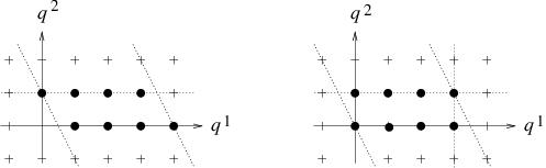
The key point is that, in any phase, any brane can be written as a complex of Wilson line branes with from either one of the two sets, by using D-isomorphisms in that phase. For example, in Phase III where the deleted set is one can use the D-isomorphisms
to bring any into the finite set. Once that is done, the brane can be transported safely along the respective route. Since the finite sets of charges are equal for the routes IIIIII and IIIIVI, the transports result in the same brane. The set is different for the route IIIIII and hence the map of branes is different.
The fact that the two routes, IIIIII and IIIIVI, give rise to the same map of branes may imply that these routes are homopotic to each other. Indeed they are! To see this let us look at the windows , and for these routes. Fig. 27 shows the overlap of these windows.

Comparing with Fig. 4, we find that the overlap precisely matches with the complement of the Alga of the singular locus . Note that any point of the alga complement determines a global section of the entire plane of FI parameters to the Kähler moduli space . Such a section defines a homotopy of the two routes under consideration. On the other hand, the overlap of the windows , and is contained inside the Alga of . This means that the attempted homotopy of the routes IIIIII and IIIIVI will intersect with the singular locus and cannot really define a homotopy.
These observations have some significance on D-brane transport along paths through the central region of the moduli space , as will be discussed in Section 8.5.
Transport Of The Fractional Branes
Let us transport the fractional branes of the orbifold along the route IIIIII. As remarked above, we can use the grade restriction rule , for this path. Recall that the fractional brane is given by
where is the defining representation. The other ones are the tensor product of this complex with . As a lift of to the linear sigma model, we may take given by
where we use “” for and “” for . The lifts of other branes can be obtained by tensoring with if and with if , with . We denote such lifts by .
Before transporting it to Phase I, we have to grade restrict the branes. That can be done simply by multiplying appropriate powers of and to the arrows. We denote this grade restricted version of by . For example, for the brane we replace the upper-right entries , , by , , and replace the ’s that go into them by . Also, we replace the rightmost entry by and substitute the arrows , going into it by , . Thus, is given by
Once that is done and the D-brane is transported into Phase I, we simply go to the low energy theory, replacing by . That’s all.
However, just as in Example (A), we may simplify the image D-branes in the large volume phase. The strategy is the same: We present the grade restricted lift as a bound state of and another brane that is infra-red empty in Phase III. Once transported into Phase I, then, this time the part is infra-red empty and we are left with . For example, described in the previous paragraph can be presented as the bound state of and
by the map that sends the bottom line of with entries to the upper-right line of by the identity maps. Note that is infra-red empty in Phase III since it consists of -Koszul and -Koszul complexes. This is why we can replace with the above bound state (which we denote by ). On the other hand, is infra-red empty in Phase I with since it consists of -Koszul complexes. Thus we find Note that also includes a -Koszul complex as a part. Dropping them, we are left with
This is quasi-isomorphic to the sheaf supported at the exceptional divisor . In this way we find that the large volume image of the fractional brane is the D-brane wrapped on the divisor with a trivial line bundle. Repeating the same procedure we find simple representatives of the large volume images of all the fractional branes :
where are the complexes of vector bundles given below.
| (8.79) | |||
In particular, the images are complexes of sheaves supported at the divisor (the pushforward of the complex over by the embedding map ).
The complexes for high values of can be simplified using the - and the -Koszul complexes. In particular, there is a duality relation
where is the transpose of the complex in which the dual of the R-degree zero component is defined to have R-degree zero. The Chern characters of are
| (8.144) |
Here and are the first Chern classes of and and is a volume form of the toric variety . They obey homology relations , , and .
(D) Resolutions Of Singularity
As the final example, we consider resolutions of the singularity, which provide historically the first example of McKay correspondence. We are particularly interested in connecting the orbifold phase and the fully resolved phase via some other phases corresponding to partial resolutions. See Section 4.4 for the labelling of phases and remarks on the phase boundaries. We consider a route that goes through the particular sequence of phases:
We see that there are phases and phase boundaries. The first phase boundary corresponds to blowing down (up) the right most divisor . Applying the general rule, we see that the phase boundary in is a domain in the hyperplane spanned by the charge vectors of all ’s but . The unbroken subgroup is therefore . At the -th phase boundary, change occurs at and the hyperplane is spanned by all ’s but . The unbroken subgroup is
which has width . Thus, the band restriction rule at the -th phase boudary is
There is a non-empty region of the space of theta parameters such that the following set of charges are band restricted at all the phase boundaries.
| (8.145) |
( is the charge vector where all but .) For example check the value (). At each of the phases on the route, any brane is D-isomorphic to a complex of Wilson line branes with charges in this finite set . For example, at the orbifold phase, all the equivariant line bundles can be realized as the low energy images of , where it is understood that . Thus, we can use this set to define the grade restriction rule for the transport of D-branes along this route, say from the orbifold phase to the fully resolved phase.
Let us see the large volume images of the fractional branes :
Its lift such that all the charges are from the set (8.145) is
where
For the case, we set so that and while and remains valid. The large volume image is obtained simply by replacing by . As before, we can simplify this image by taking out and eliminating infra-red empty complexes. For the case, we take out and eliminate a Koszul complex for a pair of variables which cannot vanish in the large volume regime. This shows that the large volume image of the fractional brane for the trivial representation is
| (8.146) |
This is the structure sheaf of the entire exceptional divisor . For , we take out three Koszul complexes associated with three pairs of variables, , and , which cannot vanish in the large volume phase since the sets with are deleted. In this way, we find the following large volume image of the fractional brane for the -th representation
| (8.147) |
This is a sheaf supported at the component of the exceptional divisor, shifted by to the left. Thus, we very explicitly recontructed the original McKay correspondence — one-to-one correspondence between the non-trivial irreducible representations of and the irreducible components of the exceptional divisor of the resolution of the singularity.
8.5 Center Of Multiparameter Moduli Space
In models with higher rank gauge groups, , we have so far discussed D-brane transport across phase boundaries only in the asymptotic regions where all but one subgroup is completely broken. However, it is of course an important problem to construct a parallel family of boundary interactions over the central region of the moduli space where multiple phase boundaries meet. Although we do not attempt to find a general solution in this paper, we have something to say about this problem.
We made an interesting observation in the two parameter model (C): There is a finite set of Wilson line branes which obeys the band restriction rule at all the phase boundaries, with the following properties;
- (i)
In each phase the set is maximal generating, that is, there is no low energy D-isomorphism relation among the Wilson line branes in the set and any brane is D-isomorphic to a complex of sums of them.
- (ii)
The overlap of windows for which the set obeys the band restriction rule precisely matches with a copy of the complement of the Alga of the singular locus , that is, the values of the theta parameters that are missed by .
The property (ii) means that the region in the FI-theta parameter space does not meet the singular locus. Due to the flatness of our connection, the outcome of D-brane transport from one phase to another, along any path inside this region, is the same as the result of transport along paths that stay in the asymptotic region. This tempts us to ask: do the Wilson line branes in this set define smooth families of boundary interactions over the entire region ? Can we use it to construct the parallel family of an arbitrary brane over this central region? In fact, existence of such a finite set of Wilson lines is not limited to the example (C) but holds in many multiparameter models. Thus, let us discuss this question in a general context of gauge theory with matter fields with charge (, ).
Let us look at the effective boundary potential on the Coulomb branch. Introducing , it is written as follows:
This is not valid on the complex hyperplanes where the -th field becomes massless, and there is also a singularity at the real hyperplanes , where the -th field has a normalizable zero mode localized at the boundary. We shall call the latter the singular hyperplanes. We would like to find a Lagrangian submanifold that asymptotes to Lagrangian planes on which the boundary potential is bounded below. Also, we would like the Lagrangian planes to avoid meeting with the singular hyperplanes as we vary the FI and theta parameters. Can we find such a family of Lagrangians? This problem is technically complicated. So let us simplify the problem by choosing a particular Lagrangian submanifold
| (8.148) |
Is the boundary potential bounded below on this submanifold ? Note that it has no danger of meeting the singular hyperplanes. On this Lagrangian plane, the effective boundary potential is given by
| (8.149) |
This is a piecewise linear function which has corners at the hyperplanes . It is bounded below if and only if it is bounded below at each one dimensional intersection of hyperplanes . Note that such a one-dimensional intersection is the direction of the subgroup which is unbroken by the values of , namely the unbroken at the phase boundary spanned by the charge vectors of these fields. And the boundary potential (8.149) restricted on that line is the same as the boundary potential for the theory of that gauge group only. Therefore, the boundary potential (8.149) is bounded below for some values of the theta parameters if and only if the band restriction rule is satisfied at all the phase boundaries for those values of the theta parameters. Under such a circumstance, we have a smooth family of Wilson line branes over the entire space of FI-parameters .
This is exactly the situation we had in Example (C). Moreover, we have a set of such Wilson line branes with the property (i). Thus, indeed we can construct the parallel family of an arbitrary brane over the central region of the moduli space, using this set just like the grade restricted set in one-parameter models.

As mentioned above, there are many other models with such a finite set of Wilson line branes. To see just one, let us take the two parameter model in Example (D) — the singularity and its resolutions. In this model, there are two sets of different kinds. One is and the other is . In Figure 28 we show the overlaps of the windows at all the phase boundaries for which the sets obey the band restriction rule. We see that they are non-empty, and moreover coincides with a copy of the complement of the Alga of the singular locus which is shown in Figure 6 (right). In fact, within two parameter models, it is difficult to come up with a model which does not have such a finite set. This makes us wonder if this is a general phenomenon. Is there always a finite set with the property (i) and (ii)? Can we always define D-brane transport across the center of the moduli space, with the simple boundary condition (8.148)?
The first counter example was shown to us by Mikael Passare. It is a theory with the following matter content:
| (8.150) |
It is straightforward to check that there is no finite set of Wilson line branes which satisfies both of the properties (i) and (ii), and that the Alga indeed has no complement. This model is actually a truncated version of a model with more parameters — the five parameter model of the singularity: the gauge theory with seven fields as shown in (4.21). If we are in a phase where , and are among the deleted set, then we obtain the same theory as (8.150) by eliminating the three variables and . By a direct computation, one can show that a set with the properties (i) and (ii) does not exist in the full gauge theory either. This example shows that we cannot always define D-brane transport across the center of the moduli space with a finite set of Wilson line branes, at least with the simple boundary condition (8.148). In such a model, a more general boundary condition is needed.
However, as an interesting observation, we would like to point out that there is a finite set of Wilson line branes with just the property (i) in all the examples we considered so far. For example, in the model of the singularity, the set given in (8.145) is maximal generating in all the phases.
We emphasize that the problem we have discussed in this subsection has nothing to do with finding a correspondence between D-branes at different phases — We had established a completely general contruction of D-brane transport between arbitrary pair of phases, using paths which stay in the asymptotic region. The main point of the present discussion was how to cover the central region of the moduli space. We found that there is a simple way to do so, provided that there is a finite set of Wilson line branes with the properties (i) and (ii). Such a set exists in many examples, but not always.
9 Some Mathematical Background
Before taking the next step into models with superpotentials, we would now like to pause to explain some mathematical background that will shed light on the previous discussions and facilitate the subsequent ones. We shall be exploring the relation of holomorphic line bundles, or more generally coherent sheaves, to modules and a simple construction of D-brane categories which follows. We use the linear sigma model as our guide throughout. The discussion in this section is a mixture of review material, some new approaches to existing results and also some original material.
Consider the manifold with coordinates . The main object of our discussion will be the ring of polynomial functions on , written as
| (9.1) |
Many geometric properties of the space have a natural algebraic description in terms of the ring .
Points of are in one-to-one correspondence with maximal, prime ideals of . For example, the point corresponds to the set of polynomials which vanish at . This set of polynomials is an ideal of since it is closed under addition and also under multiplication by arbitrary polynomials in . (It is prime since multiplying two polynomials from outside the set stays outside and maximal since it is not a subset of any bigger prime ideal — just as a point is indecomposable and minimal among complex (algebraic) subspaces.)
We are interested in D-branes or sheaves on . The simplest example is the space filling brane given by the structure sheaf . On an open set of , the local sections of are given by holomorphic functions with no poles inside the set. (More precisely, in the current algebraic context we should restrict to rational functions (ratios of polynomials) with no poles in the open set.)
The global sections of this sheaf (or any other sheaf on ) form a module over . This simply says that we can add global sections and multiply them by polynomials. In the special case of the structure sheaf, , the global sections are rational functions on the whole of , i.e., they are just polynomials. Thus the structure sheaf corresponds to the module itself, which is the simplest example of a module over .
Ideals of provide a richer class of -modules. In particular the maximal, prime ideals , discussed above, give rise to -modules for each point of . We can also consider the cokernel of the map which embeds in to form a further class of modules . These correspond to the structure sheaves of points (D0-branes) of as can be confirmed by comparing the action of on global sections of the sheaves. (Polynomials in the ideal annhilitate the module just as polynomials vanishing at act as multiplication by zero on the D0-brane at .)
There is more to say here — such as how the local sections of a sheaf can be recovered from the corresponding module (by localizing the module on the ring of polynomial functions which have no zeros on the relevant open set) — but we refer elsewhere for details [84].
We have touched on an important point above which is that given a map between modules, we can always form its cokernel and kernel which are themselves modules. This property means that the set of -modules forms an abelian category. The same is true (by definition) for coherent sheaves on .
The key result for our purposes is the following: i) the set of coherent sheaves on is in one-to-one correspondence with the set of -modules and ii) the set of maps between a pair of sheaves is identical to the set of maps between the corresponding modules. More precisely the category of coherent sheaves on and the category of -modules are equivalent as abelian categories.
We shall elaborate more on this below but roughly the statement says that on a simple enough space such as , we can learn everything about sheaves by studying global sections. This is an enormous simplification!
The lesson of the linear sigma model approach, in this context, is that we can go a long way by working with simple spaces. The remaining ingredient which we need in order to go further is gauge symmetry.
9.1 Action On — Grading Of The Coordinate Ring
In this section we will be describing a construction, due to Serre [85], of sheaves on in terms of graded -modules. Consider the action on
| (9.2) |
This induces a -grading on the ring such that the grading (degree) of a ring element is given by its representation under . Thus the degree zero elements are complex numbers, the degree one elements are homogeneous linear polynomials in the and so on.
To mod out by , we simply restrict to graded -modules and consider only maps of degree zero between modules. (A graded module of a graded ring is simply a module with a grading such that multiplication by respects grading in the obvious way.)
To find the graded -module corresponding to a particular sheaf we start as before: the degree zero elements of are given by the global sections of . However, this information alone will no longer be enough to reconstruct as a sheaf. To see this, consider the structure sheaf on , whose global sections are -valued constants. On a local patch, there are further gauge invariant sections which are rational functions of degree zero, realised as a ratio of homogenous polynomials of degree . In order to retrieve these extra local sections it is clear that we will need to keep also ‘global sections of degree ’ when we construct the module . More precisely, these are the global sections of tensored with . These provide the degree elements of the associated module .
In this way it is clear that the structure sheaf on is once again associated with the module , considered as a graded module over the graded ring . Other sheaves can be identified with graded modules in the same way.
We have given a simple description of coherent sheaves on , as graded -modules. The remaining detail to take care of is the deletion of the origin, , so that we move to . We would like to think of two sheaves as being the same on if they disagree only at the origin of . Thus, we would like to mod out by sheaves with support at the origin of .
Let us examine the structure sheaf of the origin in a little more detail. This corresponds to the graded module given by just the degree zero part of . As a vector space this module is isomorphic to and this is how we shall refer to it. The -module is annihilated by , the set of all positive degree elements of (the set of all polynomials that vanish at the origin.)
There are various other modules which are annihilated by , or more subtlely, by higher powers of . In the former class, we can consider the module shifted in degree so that it lives in degree . This module is usually labelled since it corresponds to the structure sheaf of the origin tensored with . In the latter class, we could consider for example the module given by all the degree zero and degree one elements of . We might label this module as , consisting of polynomials of degree . Clearly this module is not annihilated directly by but is annihilated by and thus should also correspond to a sheaf which vanishes away from the origin (otherwise we should be able to construct arbitrary degree polynomials in which do not annihilate the sheaf.)
In general, it should be clear that graded -modules which are localized at the origin correspond to modules whose grading is bounded above. These modules (and only these) will be annihilated by sufficiently high powers of . These form the subcategory of (graded) torsion modules and it is these that we should mod out by in order to recover sheaves on . Modding out by torsion modules simply means that we consider two graded modules as being the same if they agree for sufficiently high degree.
We are now ready to state Serre’s classic result: the category of coherent sheaves on is isomorphic as an abelian category to the category of graded -modules modulo torsion modules.
9.2 Generalization To Toric Manifolds
The generalization to toric manifolds is straightfoward. Following the route suggested by the linear sigma model, we construct toric manifolds as quotients of by , where is some deleted set. The action on gives rise to different gradings on and we consider modules which are graded with respect to all gradings. (In particular, maps between modules should be degree zero with respect to each grading.)
Dealing with the deleted sets in the different phases appears more complicated but in fact turns out to be just as simple as for . First, note that in general we want to consider -gradings on rather than just -gradings as before — in other words, some of our coordinate fields, , may have negative charges with respect to any subgroup . Associated with a single gauge group, we may consider both -torsion and -torsion modules, i.e., modules with bounded above or bounded below grading, respectively.
In each low energy phase of the linear sigma model we shall be deleting the set of points where either all positively or all negatively charged fields under particular ’s are set to zero. (Recall the description of the deleted set given in Section 4.4.) In terms of modules this amounts to moding out by either -torsion or -torsion modules under the corresponding gradings. These are the modules whose supports lie in the deleted set .
At this point we have reached a very simple unified description of sheaves in the various phases of a linear sigma model. To summarise: the category of coherent sheaves in each phase is equivalent, as an abelian category, to the category of multi-graded -modules modulo a particular set of torsion subcategories associated to .
This generalization of Serre’s construction was originally given by Cox [86] in the case where the quotient is smooth. When it has (orbifold) singularities, the above description is simply wrong if we regard as an algebraic variety, as shown in [86] with an explicit example. As discussed in Section 4.2, we do not really have a convenient description of the low energy theory unless is a smooth manifold or a global orbifold, and there is no physical reason to believe that we should take coherent sheaves of as an algebraic variety as the data for D-branes. Rather, we understand the theory as the low energy limit of our super-renormalizable gauge theory. As such, we should take -equivariant coherent sheaves over as the D-brane data, and we are indeed doing so in the above discussion. Mathematically, the category of such objects is known to be equivalent to the category of coherent sheaves on the so-called quotient stack [72]. (This last reference also gives a description of sheaves as graded modules mod torsions.) Thus, in the above statement, “coherent sheaves” should be understood as those on the quotient stack.
In the next subsection we will introduce complexes and a description of the derived category which turns out to be very simple in this setting. This will lead us to a straightforward argument that the derived categories of the different phases are in fact equivalent in the Calabi-Yau case.
9.3 Complexes
So far we have been discussing branes corresponding to individual sheaves and their description in terms of modules. We now wish to discuss more general brane configurations consisting of complexes of sheaves. In fact, since we already have an equivalence between sheaves and modules we might as well carry out the discussion in terms of complexes of modules.
We start once again with the case of where things are particularly simple. We will see that by representing arbitrary complexes in terms of ‘free resolutions’ there is no need to introduce any of the complications of the derived category and in particular no need for nontrivial quasi-isomorphisms. All branes on can be represented as complexes of free modules and in this representation, the morphisms (chiral ring elements) between branes are just ordinary -cohomology classes where represents the operator induced from differentials of the complexes.
A free -module, is a direct sum of copies of . Every -module has a surjection from a free module onto itself for some . To produce such a surjection we simply choose a generating set for the module and map the unit of a different copy of onto each generator, much as we would do for a vector space. The difference from the case of vector spaces is that there will in general be relations between the generators. We can express these relations by writing the kernel of the surjection to form a short exact sequence:
| (9.3) |
(Note that to avoid clutter we do not write explicit names of maps on arrows unless needed for clarity.) We can now start again and take a surjection from a free module onto , with kernel
| (9.4) |
If we combine the surjection from onto and the injection from into into a single step then we form a single exact sequence as the reader should verify
| (9.5) |
Continuing in this way, taking surjections from free modules onto the successive kernels we finally achieve a free resolution of (the fact that this process terminates in a finite number of steps is a result of Hilbert’s syzygy theorem)
| (9.6) |
Stepping ahead a little, we should think of this as giving a representation of as a complex of free modules in the derived category of -modules. We would now like to do the same for an arbitrary complex of -modules
| (9.7) |
We present the argument for a complex of lengh two but the generalization should be clear. We know that for and individually we can construct free resolutions
| (9.8) |
| (9.9) |
We have changed notation so that the ’s and ’s are all free modules of the form for various values of . We have also assumed that the two resolutions are of the same length (otherwise we can always pad the shorter one with zeroes at the beginning).
So to begin with, let us ‘turn off’ the map between and , allowing us (trivially) to build the following exact sequence in which all the maps are taken from (9.8) and (9.9) above
| (9.10) |
Next we would like to turn the map from to back on. We will need to simultaneously turn on some maps from the ’s to the ’s in (9.10) so that we still get a complex (i.e., so that the differential still squares to zero.)
| (9.11) |
To see that extra maps from to will be necessary just inspect the rightmost part of the diagram and notice that the two-step map from to through will not be zero in general. To correct this we introduce a compensating map from to through .
As we now explain, the property of which allows us to construct this compensating map, is that it is a free module. Suppose for simplicity that is equal to . To completely specify a map from to another module it is sufficient to specify the image of the generating element of .
Consider the map and suppose . Since maps surjectively onto , we must have some such that . Then if we map as our map from to , we can cancel the unwanted contribution. The generalization to construct (9.11) is straightforward using the fact that all are free.
Once again, there is an interpretation of the free resolution (9.11) in the framework of the derived category. As previously noted, the resolutions of and individually correspond to representations of these modules in the derived category by complexes of free modules and . Similarly, we should think of the combined complex with ‘bound’ to by the additional maps introduced in (9.11) as being an equivalent representation of the object in the derived category.
We have now described something quite interesting: every object in the derived category of -modules can be represented as a complex of free modules. This is a nice result on its own since it means that to describe arbitrary D-branes on it is sufficient to use complexes built only out of copies of the structure sheaf .
To go further, we would like to describe the space of chiral ring elements. In fact, this is where we really benefit from writing things in terms of free modules. Working with complexes of free modules, there are no non-trivial quasi-isomorphisms to worry about and all morphisms between complexes are just ordinary -cohomology classes. We shall now sketch a proof of this statement.
First we show that there are no non-trivial exact sequences built out of free modules only, or more precisely that any such exact sequence is a direct sum of trivial exact sequences of the form
| (9.12) |
where the map in the diagram above is the identity. To see this it is once again sufficient to look at the generators . Suppose we have an exact sequence of free modules and, for simplicity, suppose that the ‘rightmost’ non-zero module is a single copy of . Since this is the rightmost module in an exact sequence, the map onto it must be a surjection and in particular the generator must have a preimage. This preimage can only be the generator of the corresponding preimage module and this assures that the map is in fact (a -valued multiple of) the identity as in (9.12). The generalization when the rightmost module is is straighforward.
Given this property, it then follows by standard arguments11 1 See for example Lemma 1.6 in [87]. that all morphisms in the derived category between complexes of free modules are represented by ordinary cochain maps modulo homotopies (i.e., -cohomology classes.)
This result concludes our rather lengthy review of the derived category of ! We have seen that this derived category is in fact a very simple beast, being equivalent to the category of complexes of free -modules with morphisms given by ordinary -cohomology classes. We would now like to extend some of these results to the graded case and use them to describe branes in more interesting spaces than . We will find that some of the nice properties of free modules are lost when we mod out by torsion. The resolution to these problems is intimately related to the grade restriction phenomenon which we have already encountered in the physical setting.
9.4 Graded Case
Some parts of the analysis of the previous section generalize immediately to the graded case, in which we treat as a graded ring and allow only degree zero maps between graded modules. It remains true that given a graded module , there exists a surjection from a free module onto . However, in this case the set of free modules is richer since we need to take into account the grading. We label by the free module which is isomorphic to except that the unit is in degree . In the case of this corresponds to the sheaf . A general free module is a direct sum of one-dimensional modules of this type. (In the multi-graded case we have one-dimensional modules labelled according to the degree of for all gradings.)
Whilst switching to graded modules presents no new difficulties, modding out by torsion modules does introduce complications. The prime difficulty arises because there now exist non-trivial exact sequences of free modules. This will invalidate our argument that morphisms between complexes are ordinary -cohomology classes. Furthermore, the non-trivial exact sequences which appear will depend on which phase we are in, so that an equivalence between phases might appear unlikely. As we shall see, grade restriction provides a route around the problem. Before we demonstrate the solution, we should first take a closer look at the problem.
As an example, we set and consider the ring with degrees . (We have chosen an example in which the charges sum to zero for later convenience, but for the current discussion this is not important.) We consider the phase in which we mod out by modules with bounded above grading. Thus we are deleting the set and considering branes on .
In order to find a non-trivial exact sequence of free modules after modding out by torsion modules, we can proceed as follows. First, take a sheaf which is supported on the deleted set (a -torsion module) which will be identified with zero after modding out. The simplest example is the structure sheaf of the deleted set, which corresponds to the module (i.e., the module consisting of polynomials of only). This module is annihilated by ring elements containing any of the positively charged fields . We may also consider a version of this module shifted in degree, . For the moment let us choose .
The idea is to take a free resolution of this module as we have described earlier. When we then mod out by torsion, the original module gets deleted and we are left with an exact sequence of free modules. Here is the (minimal) free resolution:
| (9.13) |
which turns into an exact sequence of free modules after modding out by torsion
| (9.14) |
In the other phase of the model we mod out by -torsion modules, i.e., those with bounded below grading. This corresponds to deleting the set and studying branes on . In this case, the structure sheaf of the deleted set is represented by the module , which has free resolution
| (9.15) |
leading to the exact sequence of free modules (after modding out by -torsion):
| (9.16) |
We have found different ‘relations’ between free modules in the two phases which would be expected to lead to different derived categories. We shall return to this problem in the next section but first conclude this discussion with a couple of positive remarks.
Objects in the derived category modulo torsion modules can be represented as ordinary complexes of graded -modules. In other words we can pick a representative of each torsion equivalence class, which is an ordinary complex of modules (by ‘cutting off’ the modules in the sequence below a sufficiently high degree.)
Furthermore, the isomorphisms which we previously used to represent complexes of arbitrary modules as complexes of free modules, are still available to us. We should think of the process of modding out as just adding some new isomorphisms, in which case we have not changed the set of underlying objects or lost any of the original morphisms. Thus, the conclusion that objects of the derived category can be represented as complexes of free modules remains true. This is a remarkable statement and so we repeat it: any object in any of the low energy phases of the linear sigma model can be represented as a complex of free -modules.
Thus the boundary conditions we constructed earlier are the most general that we need to consider in order to describe a general brane configuration. All of the discussion so far applies equally well to the multi-graded case.
Next we would like to learn more about the morphisms in the different phases in order to study equivalences between phases. In the case we will surprisingly find a complete description of the set of morphisms in terms of an ordinary -cohomology of maps between complexes of (a restricted set of) free modules, whilst in the case we will not be able to be so explicit. In either case, the analysis will be sufficient to prove equivalence of the derived category of the different phases under the Calabi-Yau condition. The new ingredient that we shall need is grade restriction.
9.5 Grade Restriction
We start by examining the origins of grade restriction in the model of the previous subsection. The essential cause of our problems is that we have kept too many free modules of the form . In order to describe general elements of the derived category in a ‘nice’ way we need to employ a reduced set of free modules.
The basic problem shows up in terms of relations (exact sequences) between free modules. We have seen examples of this, in (9.14), relevant to the phase and in (9.16), relevant to the phase.
The existence of these relations is not only an inconvenience, but is also an obstacle to proving equivalence between phases. This is because, as illustrated in the two examples above, the available relations depend on the choice of phase.
This is where the grade restriction comes to the rescue. In both of the cases descibed above we have a relation between and a complex of modules from the set . If we restrict to the set of free modules then we claim i) to have no notrivial relations (in the shape of exact sequences) between this restricted set of free modules and ii) to have just enough modules to generate the most general object in the derived category. These statements are supposed to hold in either phase.
It is easy to convince oneself of statement i) - essentially that (9.14) and (9.16) are the ‘minimal’ relations possible in either phase. A proof can be provided, for example, by the explicit computation of Ext groups on projective space in arbitrary dimension.
So we focus on statement ii). The claim is that an arbitrary element of the derived category in either phase can be represented as a complex of free modules from the set (In general if the sum of positive charges of the coordinate fields is we restrict to the set .)
We have already seen that any object in the derived category can be represented as a complex of free modules if is allowed to take arbitrary values. So roughly, we need to show that any free module can be expressed in terms of the restricted set .
The idea behind this is quite simple. Suppose we are in the phase. We may use relation (9.14) to write in terms of the restricted set. Recall that in the derived category this exact sequence should be thought of as an equivalence between and the complex
| (9.17) |
Next we consider . We may use (9.14) shifted in degree in order to write in terms of
| (9.18) |
To write in terms of the grade restricted set, we may then replace each of the ’s by modules from the restricted set, as above.
To do this explicitly we want to ‘bind’ (9.18) to three copies of (9.14) and then ‘annihilate’ pairs of ’s. We show how to bind to the first copy of (9.14).
Consider the identity map from one of the ’s in (9.18) to in (9.14). We claim that this map can be extended to a map between complexes. (Note that we are talking here about an honest cochain map between complexes of modules rather than some more general morphism in the derived category in which case the statement would be trivial.)
| (9.19) |
Every map in this diagram is an honest map between modules and the whole argument can be carried out even prior to modding out by torsion. However, in that case, the complex (9.14) represents a non-zero module and so the object (9.19) produced after binding would not be equivalent to (9.18). Once we mod out, the operation becomes an equivalence since we are binding to an object with support on the deleted set.
To construct the cochain map used above, we use a small extension of the argument we gave earlier in the construction of equation (9.11). That construction allowed us to build a map from a complex of free modules to an exact sequence of modules. In the current situation, we want to build a map from a complex of free modules (9.18), but in this case the complex we are mapping to fails to be exact in the rightmost position (as a complex of modules prior to modding out.) However, the failure of exactness is only in the lowest degree and does not cause a problem since the maps to in (9.18) are all at least linear in the positively charged fields. We leave it to the reader to check the details.
The ‘annihilation’ step is to remove the trivial pair from (9.19), to leave an equivalent complex in which we have reduced the number of ’s
| (9.20) |
By repeating twice more for the remaining ’s we finally write as a complex of modules from the grade restricted set.
It should be clear how to extend this argument for , by induction. More generally, given any object in the derived category, represented as a complex of free modules, we can remove step-by-step all of the modules with by repeating this construction many times. (At each step we remove the remaining free module of highest degree which is positioned furthest to the right in the complex so that all maps to this module are at least linear in the positively charged fields and we can argue as above.)
For with there is a similar argument using the sequence (9.14) shifted in degree by and read from left to right as a relation between and the restricted set. Once again, by shifting degrees and iterating, we may extend this argument to the general case of . The binding process in this case involves maps from shifted versions of (9.14) to the complex that we are grade restricting. To construct the relevant maps we can use a trick of ‘dualizing’ to put ourselves in the situation above, applying the binding procedure above and then dualizing back. Dualizing in this context means replacing all free modules by and reversing the direction of all maps.
This completes the proof that all objects in the derived category in the phase can be written as complexes of grade restricted modules. The same argument holds in the phase although in this case it is rather more straightforward to see since according to (9.16), every pair and are isomorphic and so we can always replace with mod . Also, although we treated a specific example, the same arguments work just as well for the general linear sigma model. We are now ready to state our general result:
Suppose we have a linear sigma model with positively charged fields and negatively charged fields , such that the sum of charges of the is and the sum of charges of the is . Let be the associated graded polynomial ring.
The model has two low energy phases. In the first phase, which corresponds to deleting the locus the branes are given by the derived category of graded -modules modulo those with bounded above grading. Every object of this category can be represented as a complex of free modules from the grade restricted set . Furthermore, morphisms in this representation are ordinary cochain maps modulo homotopies (-cohomology classes) and there are no non-trivial quasi-isomorphisms.
Similar statements hold for the second phase and the general brane in this phase can be written as a complex of free modules from the grade restricted set . In the Calabi-Yau case, , this gives an explicit equivalence between the derived categories of the two phases.
Parts of this result have appeared previously in the literature. For the case of , the description of an arbitrary brane as a complex of follows from Beilinson’s work [88]. The equivalence for and is a special case of the McKay correspondence by Bridgeland-King-Reid [6], as already mentioned in Section 8.4. Bondal-Orlov [89] and Bridgeland [79] studied cases where all fields have degree and proved equivalence between phases under the Calabi-Yau condition.
A. King pointed out to the authors that the result as stated above appeared previously in a work by Van den Bergh, see [90] Section 8. Thus, we cannot claim it as our own original result, even though we were not aware of that work at the point we obtained it. Nonetheless, our approach to the problem, based on the physics of linear sigma model, naturally leads to a number of important generalizations. One of them is generalization to multi-graded cases, which we discuss next. Another is extension to systems with superpotential, which we will discuss in Section 10, where we obtain equivalences of the derived category of a Calabi-Yau manifold and different type of triangulated categories, such as the category of matrix factorizations. All these equivalences are unified under the same principle — the grade restriction rule.
9.6 Multi-Graded Case
We would like to describe the effect of crossing phase boundaries in the general linear sigma model. Since only a single is unbroken at each boundary, we already have all the necessary tools at our disposal.
We write the general one-dimensional free module as to display the grading under each . We focus on the first and suppose that the sum of positive (resp. negative) charges of the variables under this is (resp. ) as before.
Suppose that we are in a phase in which we need to mod out by the -torsion modules (those whose grading is bounded above under this ). According to our previous discussion, we can describe an arbitrary brane in this phase as a complex of free modules , where can be restricted to lie in the range . We treat phases in which the D-term for this takes the opposite sign in a similar way — restricting to lie between and .
Since we still have to mod out by torsion modules for the remaining ’s, we expect to have relations (in the form of exact sequences) between the set of free modules for which only has been grade restricted, i.e., relations within the band restricted set. Thus, we can no longer claim to have a simple description of the derived category in which morphisms are ordinary -cohomology classes (homotopy classes of cochain maps). However, for the purposes of describing equivalences between neighbouring phases this is not necessary. This is because when we move between adjacent phases, we only switch the sign of a single D-term and so switch from -torsion to -torsion for a single . The remaining ’s are not affected, and hence modding out by remaining torsion modules is the same procedure for both phases. This is manifest in the relation (4.22) between the deleted sets.
Thus it becomes clear how we are to compare branes in different phases. Each time we wish to cross a phase boundary we grade restrict with respect to the associated . We may then pass freely into the next phase. If the sum of positive and negative charges of the variables are equal for the in question, there will be no new relations between branes after crossing the boundary and we will have an equivalence of categories. If the Calabi-Yau condition (4.15) holds so that the sum of charges is zero, then it follows, by crossing a boundary at a time, that the derived categories in all low energy phases are equivalent.
We emphasize again that, unlike in the single graded case, this proof of equivalence does not imply nor rely on a simple description of derived categories in terms of a finite set of rank one free modules. In fact, there is a toric variety which does not admit such a set (the counter example [91] to King’s conjecture [92]). However, as mentioned in Section 8.5, there is such a finite set in all the Calabi-Yau examples we considered so far.
A different construction of derived equivalences in the general multi-graded case had been given by Kawamata in [80].
9.7 Generalizations
Although we shall not develop these here, there are various directions in which one could generalize the preceding analysis. One possibility is to allow a non-Abelian group action on and thus decompose into representations of . This line of development has been initiated by Kapranov [87, 93] who generalizes the Belinson result for sheaves on to Grassmanians. Clearly, these developments will be relevant for describing branes in non-Abelian linear sigma models.
Another direction is to consider more general choices of the ring . Much of the basic theory can be developed even in the case of non-commutative rings [94] and it would be fascinating to develop a physical interpretation of this work. However, we leave these directions to future research and return now to our main focus which is the study of D-branes in Abelian linear sigma models.
10 Compact Models
In this section, we consider the problem of D-brane transport in systems that arise from linear sigma models with superpotential. Applying the grade restriction rule, we find a rule of D-brane transport along paths on the Kähler moduli space. This leads, for example, to one-to-one correspondences between D-isomorphism classes of D-branes in Landau-Ginzburg orbifolds and those in geometric regimes. The basic idea of transport itself is identical to the one in the non-compact models of Section 8. Besides having matrix factorizations instead of complexes, the main new feature is that, depending on the phase, some of the bulk fields may acquire masses from superpotential F-terms and therefore must be integrated out.
10.1 The D-Brane Transport
To start with, let us briefly recall the rôle of the superpotential in the bulk theory. The classical vacuum configuration in the Higgs branch is govened by the D-term and F-term contributions to the potential (4.8). Away from phase boundaries, the D-term potential confines dynamics to a toric, non-compact Calabi-Yau variety . The F-term potential determined by the superpotential restricts the vacuum further to a complex subvariety . Depending on the phase, a part of the transverse modes of in may acquire mass from the superpotential F-terms. In the case where all transverse modes are massless, the low energy theory is a Landau-Ginzburg model with superpotential over the non-compact toric variety . In the other extreme where all transverse modes are massive, we obtain a non-linear sigma model on the vacuum manifold . The nature of low energy theory depends very much on the phase and the pattern is in general very complex.
However, one could always choose to use the description as a LG model on the non-compact toric variety . This description is most natural if the energy scale, , set by the D-terms is much higher than the one, , set by the F-terms, and we consider an intermediate scale, .
Like in the non-compact situation we are taking the large gauge coupling limit, so that we can integrate out the gauge multiplet algebraically (cf. (4.12) and (4.14)). The matrix factorization in the linear sigma model then becomes a matrix factorization of over the toric variety . Let us denote the set of matrix factorizations of over by , and refer to the set of matrix factorizations in the linear sigma model as . Two D-branes in that are related by D-isomorphisms will flow to the same D-brane in the infra-red limit, so that we define as the set of matrix factorizations of the linear sigma model up to D-isomorphisms. Let us introduce the corresponding projection:
Similarly to Section 8.1 we have a pyramid of maps:
| (10.1) |
Let us illustrate these projections in Example (A) with . We pick the superpotential with the cubic fermat polynomial . In the limit, this gives the LG-model with superpotential over the orbifold , namely, a LG orbifold. At and at the intermediate energy scale we have a LG-model with potential over , the total space of the line bundle . This superpotential gives masses to the fibre coordinate and to the transverse mode of ’s to the hypersuface , but we choose to keep both of them. At lower energies , it is more appropriate to integrate them out, and we have the sigma model on the elliptic curve, .)
In order to describe D-isomorphism realtions in the two phases, we first consider matrix factorizations that are infra-red empty, i.e., the ones for which the boundary potential is strictly positive over . They can be constructed from the Koszul complexes for the deleted sets, and will play the analogous rôle as the latter played in the non-compact models. Recall that our R-charge assignment is .
In the phase, the deleted set is . Let us consider the brane given by
For simplicity, we use the following notation to encode this data:
| (10.2) |
The subscript of each Wilson line brane labels the R-charge. This brane has strictly positive potential over where is non-zero, and therefore is infra-red empty. Note that this matrix factorization is obtained from the complex , which defined an empty brane in the non-compact model with , by adding the arrow in the opposite direction, .
Let us next consider the phase where the deleted set is . Just as above, we consider adding some arrows to a complex corresponding to an empty brane in the non-compact model, such as which can be realized as on the Clifford module. If we add the arrows in the opposite direction, we find a matrix factorization of . With an appropriate choice of R-charge, say on the Clifford vacuum , we have a graded matrix factorization. Presented in the similar way as (10.2), it is
| (10.3) |
with
The boundary potential is strictly positive on , , and the brane is indeed infra-red empty in the phase.
Let us bind these two branes using a map from to :
| (10.4) |
Following the procedure from (3.15) to (3.16), which applies also to matrix factorizations, we can erase the trivial pair . The result is
or more explicitly
with
| (10.5) |
In the phase where the brane is empty, this process results in the low energy D-isomorphism
| (10.6) |
which trades the Wilson line component for . The shift in the R-charge is due to the fact that the varibale carries R-charge and that is obtained from by relocating . In general, given a matrix factorization in the Landau-Ginzburg phase, we can always eliminate the Wilson line component with largest charge in favour of , as well as the smallest charge component by . This reflects the broken gauge symmetry in the Landau-Ginzburg orbifold model, and tells us that we can simply set in order to obtain -graded matrix factorizations. In the next subsection. we will see how this works in a general model.
In the phase where the brane is infra-red empty, the above process results in the D-isomorphism
| (10.7) |
The Wilson line component in is traded for others with . Just as in this case, we can always lower (and increase) the gauge charges , by binding with or with its shifts in gauge and R-charges. Each binding process changes the charge by at most .
Grade Restriciton Rule
We now transport D-branes across phase boundaries. Let us consider two adjacent phases, say Phase I and Phase II, and fix a window at the phase boundary. The grade restriciton rule (or more generally the band restriction rule) of Section 7 tells us that we cannot transport arbitrary matrix factorizations along a path that goes through . Only those branes whose Wilson line components are contained in the band restriction rule can be transported, i.e., must be in the band . We denote the set of matrix factorizations in the band by . Just like (8.6) in the non-compact case, we can associate to a given window , a hat diagram:
| (10.8) |
The lifts and projections compose to the maps
which are inverse to each other, and . They induce a one-to-one correspondence between D-isomorphisms classes in and . The key step in the hat diagram (10.8) is the lift from the low energy matrix factorizations in a given phase, say , to the grade restricted subset . A random lift of a matrix factorization in to the linear sigma model does not comply with the band restriction rule. We can, however, bind trivial D-branes to in orde to eliminate Wilson line components outside the band, without changing the D-isomorphism class in .
In the example at hand, the trivial branes at small volume, , are the matrix factorizations
for any and . In the large volume phase, , the trivial branes are
for any and . Note that both D-branes have just the right width in the range of gauge charges in order to enable the restriction to for some window at the phase boundary. The binding process (10.4) is an example where the Wilson line component is eliminated in order to fit the matrix factorization into the grade restriction rule associated to the window . Indeed, the matrix factorization is an object in , and as a result of relations (10.6) and (10.7) we find:
| (10.9) |
Just as in this example, in any model, the trivial matrix factorizations to be used for grade or band restriction processes are obtained from the trivial complexes in the non-compact version. For the general model with gauge group (using the notation in Section 8.2), they are obtained from the -Koszul and -Koszul complexes by adding arrows in the oppostite directions
| (10.10) | |||||
| (10.11) |
Here and are such that
Since is gauge invariant, such ’s and ’s always exist if is assumed to be reduced with respect to the non-trivially charged fields (i.e. for ). We have neglected to put the R-charge information in (10.10) and (10.11).
For a model with higher rank gauge group, with , at each phase boundary we can construct similar matrix factorizations of the part of which is reduced with respect to the relevant fields at that phase boundary. Then, we can take the tensor product with any matrix factorization for the remaining part of to make a trivial D-brane. As in the non-compact version, there are amibuities in the grade restricted lifts and , but they are due to common deleted sets of the two pahses and hence do not matter in the end.
Integrating Out Heavy Fields
We have achieved our goal also in models with superpotential — we have a complete rule of D-brane transport across phase boundaries. However, the “low energy” theories in the above discussion are non-linear LG models on toric verieties , which are in general different from the typical description, such as nonilinear sigma models without potential or LG models on linear space. In order to have a useful transportation rule, we need to fill this gap.
The main gap exists in large volume phases where all the modes transverse to in acquire masses from the F-term superpotential . For scales below the F-term mass, we can integrate out these massive modes and we obtain the non-linear sigma model on . Matrix factorizations must turn into complexes of holomorphic vector bundles over . The pyramid (10.1) is then enhanced by maps in such phases, which associate to each matrix factorization at the intermediate scale a geometric D-brane on the subvariety :
We will find what the maps are, and see that they induce a one-to-one correspondence between geometric D-branes in and matrix factorizations in . Unlike in the bulk theory, where integrating out the massive fields essentially corresponds to setting them equal to zero, the presence of a boundary enriches the story significantly.
A gap also exists at Landau-Ginzburg orbifold points where the usual low energy description is in terms of LG models on linear spaces. This has nothing to do with F-terms but has to do with D-terms. At a LG orbifold point, some of the linear sigma model fields simply decouple by acquiring infinite mass from the Higgs mechanism, and we are left with the LG model for the rest of the fields. Thus, it is more convenient to use the description that includes only those massless linear fields, rather than to work with the set of all fields and implement the D-isomorphism relation, such as (10.6), all the time.
Before attacking the main problem to find the maps in large volume phases, we first fill this gap at LG orbifold points.
10.2 Landau-Ginzburg Orbifold Point
We need to establish the equivalence of the two descriptions at a Landau-Ginzburg point, one with the full set of fields subject to the D-term relation and the other with the reduced set of fields without any relation. This problem also exists in the model without superpotential , at a free orbifold point, and could have been discussed in Section 8. The treatment we will provide below can be easily adapted for that case as well, and we will leave that to the reader.
We first discuss the problem in a specific class of examples — Example (A). Once that is done, the generalization is straightforward and will be described only briefly.
10.2.1 The Theory
Eaxmple (A) is a gauge theory with fields of charge . The superpotential is where is a degree polynomial of . The limit is the Landau-Ginzburg orbifold point where has a vacuum expectation value that breaks the gauge group to the subgroup of -th roots of unity. The and the gauge multiplets decouple together by acquiring infinite Higgs mass.
Elimination Of
Elimination of is straightforward — simply set it equal to its expectation value which can be chosen to be 1. Of course, since the field carries R-charge , we must change the gauge for the R-symmetry transformation. It is done as follows.
Let be a D-brane in the linear sigma model. We set
| (10.12) | |||
is of course a matrix factorization of . It is invariant under the orbifold group action, , and has R-charge ,
The operators and of course commute and satisfy
Thus, we obtained a D-brane in the LG orbifold.
Inclusion Of
Let us next find the map in the opposite direction — from a D-brane in the LG orbifold to a D-brane in . Actually, we will be able to find a map directly into the grade restricted subset in the linear sigma model, for any window at the phase boundary. This will be particularly useful for D-brane transport from the LG point to the large volume regime. We recall that the set of admissible charges for a window is a set of consequetive integers. In particular, it has the property
| (10.13) |
Let be a D-brane in the LG orbifold. One can choose a basis in which and are simultaneously diagionalized, with eigenvalues and respectively. Here we use the indices , to label the Chan-Paton basis vectors. is a rational number and is a mod integer. Since , we find that is or depending on whether the basis element is even () or odd (). Namely, is an even or odd integer depending on or . In fact, for such an the equation
| (10.14) |
is uniquely solved by integers from the range
Let us now put
| (10.18) |
Then we have and mod , that is, for an -th root of unity . Hence, by the orbifold invariance of we have
This means that depends on only though . Since is a polynomial of ’s and since conjugation by can change the power of only at most by (see (10.13)), we find that has no negative powers of , that is, it is a polynomial in ,
is the component of such that . Now we define by replacing by :
| (10.19) |
Let us perform some checks on this . Using the gauge transformation property of , we see that the equation decomposes into the following set of equations
These are compiled into a single equation
which says that is indeed a matrix factorization of . Gauge invariance and R-symmetry simply follow from the definition,
To summarize, given by (10.18) and (10.19) has all the properties to define a D-brane in the linear sigma model. We have constructed a map that sends D-branes in the LG orbifold to grade restricted D-branes in the linear sigma model. It is clear that this is the inverse of the map which was obtained by setting and modifiying the R-symmetry by an appropriate gauge transformation.
Example
If we apply the map to the D-branes , and that were introduced in (10.2), (10.3) and (10.5), we find
where are obtained from or by setting . The subscripts are the Chan-Paton R-charges in the low energy theory. We indeed find the empty brane as the image of . Also, and are mapped to the same D-brane. (The image is equal to the Recknagel-Schomerus brane in the notation of Section 2.4.1.) If we apply the inverse map to the two LG branes obtained above, with the grade restriction rule , we find respectively
The latter is .
10.2.2 General Case
In a general linear sigma model, a Landau-Ginzburg orbifold phase occurs when the gauge group is broken to a finite subgroup by non-zero values of fields, say , and the D-term equation can be solved for arbitrary values of the remaining fields, . The deleted set is then
| (10.27) |
There is a fractional change of basis of the gauge group that brings the charges into the following form
In such a basis, the orbifold phase is . Indeed, the D-term equation can be solved at for arbitrary ’s by setting . In what follows, we use the original integral basis, with . The only thing we need to know is that the matrix is invertible over rational numbers and that are non-negative.
The low energy theory is the LG orbifold with variables and superpotential
The orbifold group consists of elements of obeying
Recall from (5.27) that the R-charges of the fields are even integers. The R-symmetry action on ’s can be trivialized by dressing with the gauge transformation where is the unique rational solution to the system of -linear equations
The R-charges of in the low energy LG model are thus
The element acts trivially on ’s, , and acts on ’s by the phase where we used the fact that the ’s and the ’s are even integers. Namely, it belongs to the orbifold group and acts on the Landau-Ginzburg fields in the same way as the R-symmetry at . Therefore, we can identify as the element that was defined in Section 2.4.1.
Elimination Of ’s
Given a brane in the theory with full set of variables, we set
| (10.28) | |||
This defines a D-brane in the LG orbifold.
Inclusion Of ’s
Let be a D-brane in the LG orbifold. We denote the eigenvalues of and as and . It follows from that is an even (odd) integer if labels an even (odd) Chan-Paton vector. Analogously to the case, we would like to find an even (odd) integer and a set of integers satisfying the equation
There is a unique solution if we require to be in a bounded range such that is in an open interval of width . Since the deleted set is the union of the hypersurfaces , (10.27), this bound precisely matches with a fundamental domain of the Chan-Paton charges with respect to the D-isomorphism relations of the Wilson line branes.
Once the solution is found for each , we define and as in the case. It follows from the orbifold invariance of that depends on only through
It is in fact a polynomial of , due to the bound on , as one can see in the fractional basis of mentioned at the beginning. In particular, one can write such that where is a -tuple of non-negative integers , and is a short-hand notation for the product . Setting
we obtain a D-brane data in the linear sigma model. We have constructed the inverse to the map in (10.28).
10.3 Geometric Phase
We now attack the problem of integrating out the bulk fields that acquire mass from the superpotential F-term. In fact, we had already considered the same problem in the context of a simple Landau-Ginzburg model in Section 3.4, where we integrated out two variables, and , which enter into the term of superpotential. We shall refer to our result of Section 3.4, given in (3.53) and (3.54), as the Knörrer map. Our current situation can be regarded as a massive LG model fibred over the subvariety , with a non-degenerate quadratic superpotential as a function of the transverse coordinates. Thus, we may simply apply the Knörrer map fibrewise in this setup.
In the first part of this subsection, we directly apply the Knörrer map and obtain the map of matrix factorizations in to geometric D-branes in . In the second part, we reformulate the Knörrer map and find the inverse map, from geometric D-branes in to matrix factorizations in .
10.3.1
We first consider Example (A) with the superpotential
| (10.29) |
The geometric phase is , and the description at the intermediate scale is the LG model with this superpotential over the total space of the holomorphic line numdle . The superpotential is critical at the submanifold , which is a degree hypersurface of the projective space . We may say that we have a LG model with superpotential fibred over the hypersurface . Thus, we can simply apply the Knörrer map fibrewise. We obviously have two options, one with the identification and and the other with and . The two must give rise to the same answer provided we do everything correctly. In this first part, we take the former option. The latter option turns out to be useful to find the inverse map and will be considered in the second part.
Let be a linear sigma model brane representing an element of . Following the Knörrer map we put
| (10.30) | |||
| (10.31) |
is regarded as acting on the infinite dimensional space . The gauge and the R-symmetry actions , on the new Chan-Paton space are naturally determined by the respective charges of , up to an overall shift ambiguity. This ambiguity is fixed by setting
| (10.32) | |||
| (10.33) |
As we have discussed in Section 3.4, we need to make a choice of the overall R-charge assignment, and (10.33) is just one choice. As for the gauge group action, on the other hand, there is no such ambiguity. We will see that (10.32) is the correct identification, as long as the B-field on is given in terms of the theta parameter by
| (10.34) |
is the data of the D-brane in the low energy sigma model. The Chan-Paton space with representations corresponds to a graded vector bundle over ; a one-dimensional subspace of of gauge charge and R-charge corresponds to a rank one subbundle of at degree which is isomorphic to the line bundle on . acts on as a degree 1 bundle map. Since we are on the hypersurface it squares to zero
Thus, we have a complex of vector bundles. Since has R-charge , the subspace for larger corresponds to a subbundle with larger R-degree. Therefore, if the original Chan-Paton space was finite dimensional, the degree subbundle has finite rank for each , and the complex is bounded from the left, but unbounded to the right;
| (10.35) |
Here is the minimum of the R-charges of . Although it is an unbounded complex, it is exact at large enough R-degrees. This follows from the corresponding property of the Knörrer map, see Section 3.4. Indeed, the infra-red empty blocks of the matrix shown in (3.55) are on subspaces of large R-charges if we assign R-charge 2 to the variable . There is also an alternative, algebraic proof of the exactness at large degrees, which will be given momentarily. In either way, we know that it is quasi-isomorphic to a bounded complex of coherent sheaves, such as
for some large .
Let us illustrate the procedure using the brane in the case, which was introduced in (10.2). The original Chan-Paton space is two-dimensional, and let us denote the basis vectors by , . The basis elements , of the new Chan-Paton space have (gauge,R)-charges , respectively and thus correspond to the line bundles , over the elliptic curve . maps the basis elements as follows
Thus, we find the complex
We find infinite copies of trivial brane-antibrane pairs. Eliminating them all, we are left with the finite complex . Hence, the Knörrer map yields
Let us consider another example, the brane given in (10.3). As above, for each Wilson line brane we have an infinite series of line bundles on the elliptic curve. We first write the entries in (10.3), from left to right with respect to the R-charge, draw the arrows from the -independent part of , and replace the notation “” by “”:
We next write its copies, shifted to the right by two and tensored by , and draw the arrows including the -dependent part of :
This is the complex . It is exact. The exactness can be proven algebraically, but one may also prove it by computing the potential and showing that it is positive everywhere: The potential is except at the first few terms, , , and , where it is , , and respectively. All the eigenvalues are bounded from below by and are positive as long as . Therefore, the brane determined by is infra-red empty, which is indeed expected from .
If we apply this procedure to the brane given in (10.5), we immediately find the complex :
Notice that it is almost the same as except for the term with a map to . Namely, it is the cone of this map:
Since is empty, we see that our brane is D-isomorphic to just which is the same as the result for . This is exactly what is expected from (10.7).
Theta Shift
We now show that the Chan-Paton gauge charges of the low energy D-brane are given by (10.32) with theta parameter shift (10.34). To this end, we put the derivation of the Knörrer map in Section 3.4 into the context of a gauge theory. Thus, we assume that the variables carry some gauge charges so that the superpotential is gauge invariant. We suppose that and have charges and respectively. Then, the boundary variables and of the brane (3.50) must carry gauge charges and respectively. Accordingly, the Chan-Paton vectors from the () sector have the following gauge charges:
| (10.36) |
Now suppose we have some brane in the low energy theory and consider the brane (3.51) in the high energy theory. If we integrate out the -system, we get back exactly the original brane since the ground state of the -system has zero effective energy and zero effective charge, see Section 6.10. Let us look into the form of Chan-Paton vectors in this context. If are Chan-Paton vectors of the original low energy brane , then the Chan-Paton vectors of the high energy brane (3.51) are of the form . If ’s have gauge charge , then the latter have gauge charges . These are the Chan-Paton charges that we see before integrating out and . The Knörrer map is the procedure that takes out . However, what we want as the Chan-Paton vectors in the low energy theory are just , but not . Thus, to find the correct charge of the low energy Chan-Paton vectors we need to subtract the charge of from the high energy Chan-Paton vectors. This yields the rule
Since the theta parameter contributes to the boundary charge in the form , one can relocate this shift to a shift of the theta parameter
now without shifting the ’s. In the current set up where and hence , this rule leads to (10.32) with (10.34).
A shift of the theta angle due to integration of massive fields was first found in the context of closed string topological A-model by Morrison and Plesser [60]. There, only the shift modulo matters and indeed their result is consistent with ours: . In the present context of (physical or topological) open string theoy with B-type boundary conditions, a shift by an integer multiple of also matters. The above result shows the precise shift, including the integral part.
Left Semi-Infinite Complexes
That the semi-infinite complex (10.35) is exact at large enough degrees can also be proven purely algebraically. The essential point is a well known fact in the theory of matrix factorizations (Eisenbud [13], Proposition 5.1): Let
be a matrix factorization of some polynomial , of size . This induces an infinite, 2-periodic complex of modules over the ring
| (10.37) |
Then this complex is exact. This is proven as follows. Suppose some homomorphism , induced by an polynomial matrix , obeys the equation . This means that the matrix is divisible by , that is, there is a matrix such that . Then we have , which means . In particular . This shows the exactness at . The exactness at the other position can be shown in the same way.
In fact, this infinite complex is the totally acyclic complex (2.72) that we met before in Section 2.4, where we studied the chiral ring for matrix factorizations. We recall that we denoted it by .
If we replace by
| (10.38) |
in the definition of for , then we obtain an infinite complex of vector bundles unbounded both in the left and right. If we regard it as a complex of modules over the ring , and if we ignore the grading, it is 2-periodic and coincides with the totally acyclic complex associated with the matrix factorization of the polynomial . In particular, it is exact and can be regarded as a graded version of . We denote it by . Our semi-infinite complex (10.35) is obtained from this exact complex by chopping off the semi-infinite part corresponding to the negative power components . This proves that (10.35) is exact at large enough degrees.
The fact that the complex is a part of the exact complex also shows that there is an alternative description: Take the remaining part (i.e. the negative power part ) and shift it by to the right. This produces a semi-infinite complex which is unbounded to the left, but bounded from the right. Of course, this left semi-infinite complex is quasi-isomorphic to the right semi-infinite complex . For example, the left semi-infinite version of the complex that represents is
If we attatch to this complex with the map from the right-most entry, , the result is an exact complex. (This can be seen by showing that the bounday potential is positive, or by noting that it is the complement of the exact complex in the exact complex .) Namely, there is a quasi-isomorphism from this complex to . Thus, we obtain again the same result for .
Complete Intersection Of Hypersurfaces In Toric Variety
It is straighforward to generalize the above construction to the case where is a complete intersection of hypersurfaces in a toric variety. Let us consider a gauge theory which has fields , with charge , , and the superpotential
| (10.39) |
where are homogeneous polynomials of degree with respect to the -th gauge group. We assign R-charges to ’s and to ’s. We suppose that there is a phase in which the gauge group is completely broken by the values of the ’s and the non-compact variety is the total space of the rank vector bundle over a compact toric manifold . Then, the low energy theory is the non-linear sigma model on the critical locus (), which is the complete intersection of hypersurfaces in the toric variety . If we have a D-brane in the linear sigma model, then the brane in the low energy sigma model is given by
| (10.40) | |||
| (10.41) |
The gauge and R-symmetry representations and are determined by the charges of ’s and by the initial condition: , in the subspace , provided the B-field is given by
| (10.42) |
The brane defines a semi-infinite complex of vector bundles over which is bounded from the left but unbounded to the right. It is exact at large enough degrees and hence is quasi-isomorphic to a finite complex. This follows from the property of the Knörrer map, but also can be shown algebraically. Indeed, if we relax the condition on the range of the sum in (10.40), for example, if we include the sum over negative as well, then we have an exact complex of modules over the complete intersection ring . To see that, just regard as the hypersurface ring of and apply Eisenbud’s proof to the matrix factorization of over the ring . In particular, we have various other versions of corresponding to various different ranges of the sum (10.40). As an example, consider the sum where all ’s run over negative integers. From this, with shift by to the right, we obtain a left semi-infinite complex that is quasi-isomorphic to .
10.3.2
We now construct the inverse map. The key is to consider the opposite identification in the Knörrer map, , . Setting is straightforward, but extracting power series of from a given matrix factorization is hardly practical. This motivates us to reformulate the Knörrer map.
Reformulation Of The Knörrer Map
The reformulation is best described using the language of rings and modules that we introduced in Section 9. Let us first describe the original formulation of the Knörrer map in that language.
A matrix factorization of the superpotential can be regarded as the pair where is a -graded free module over the polynomial ring and is an odd endomorphism of that squares to the multiplication map by . Setting corresponds to replacing by the module over the ring which is isomorphic to
The Knörrer map image is then obtained by regarding as a module over the ring which does not include the variable . If has rank over , then has infinite rank, As we have seen, this infinite-size matrix factorization is isomorphic to a finite one, which we denote by .
Now let us describe the new formulation. The key step is to view as the quotient of by the ideal ,
and to regard the -module as an -module by the rule , for and . We denote the result by . It is a matrix factorization of over . By itself, is not a free -module but one can find its free resolution, using the canonical resolution of ,
Namely, we replace each in by and add the map to . In other words, we take the graded tensor product and consider the sum . This free resolution is nothing but , if is obtained from in the way described in Section 3.4. In general, is of such a form up to the trivial matrix factorizations , , and the trivial pieces are certainly trivial even after setting . Thus, we find
| (10.43) |
This is the property that the low energy brane must have. This can be used to find the inverse map: given a matrix factorization of over the ring , we push it forward by to a matrix factorization over the ring , and then take its free resolution. The final step is to recover the variable .
Hypersurface In Projective Space
Let us apply the above reformulation to Example (A). With the identification and , the rings that appear are ,
Of course, everything is graded with respect to the gauge charge, and we also work in the large volume phase where the locus is deleted. Namely instead of graded -modules (resp. -modules) we consider coherent sheaves over the projective space (resp. the hypersurface ). In this context, the map sending -modules to -modules becomes the pushforward of sheaves by the embedding . Let be a bounded complex of coherent sheaves over the hypersurface . The first step is to push it forward to and take its free resolution. At this stage, we have a bounded complex of vector bundles over of the form
This determines the data where is a matrix polynomial of obeying
Of course, is gauge invariant and has R-charge 1 with respect to the representation of the gauge and R-symmetry group. The final step is to recover the variable , that is, to find the extension of to a matrix factorization of ,
which is gauge invariant and has R-charge . The condition can be decomposed into a set of equations
| (10.44) | |||
| (10.45) |
The (gauge,R)-charge of must be . We shall find such ’s recursively, starting with . Multiplication by defines a cochain map . Since is a resolution of the complex supported at , this map has to be null homotopic. This shows that there is a map of degree such that equals the -multiplication. Thus, we found of charge obeying (10.44). The rest of are found by induction. Suppose that we found that solves (10.45) for all below . Then
This means that is a cochain map. The degree of this map is which is negative. Since the Ext group is zero for any negative degree , the cochain map has to be null-homotopic. This shows the existence of a degree map that satisfies (10.45) for .
In this way we obtain the data of a brane in the linear sigma model. Obviously, this is the one that must descend to the complex that we started with. There is one subtlety though, concerning the value of the theta parameter and the overall shift of R-charge. The theta parameter must be related to the B-field of the low energy sigma model by
| (10.46) |
The choice of R-symmetry is a matter of convention. However, if we want to be consistent with the one in (10.33) that was used in the map , we need to replace by
| (10.47) |
To see this, let us come back to the derivation of the Knörrer map and its reformulation. The lift of a low energy brane to the high energy theory is given by and . In the discussion of the map we used the identification , while we used for the inverse map . However, to compare the two stories, it is better to use a common framework. We can actually use also in the discussion of the inverse map — we just have to change the notation as . The charge assignment for was . The gauge charge is canonical but the R-charge is a choice. This choice is the one corresponding to (10.33). Thus, in the inverse map, we must use
In view of this charge assignment, the free resolution of must be
instead of the standard one which was used above in obtaining . Thus, we must shift the charges as
| (10.48) |
The shift of the R-charge is nothing but (10.47). The shift of the gauge charge can be traded for the shift of the B-field which gives (10.46).
As an example we consider D-branes on the Fermat type elliptic curve, . We first consider the D2-brane with trivial gauge field, the structure sheaf of the curve, with some value of the B-field. Its pushforward to is the sheaf supported at , and its free resolution is given by . It is easy to find its lift to the linear sigma model:
If we apply the map to this brane, we obtain the complex on the curve ,
This is quasi-isomorphic to with and that is indeed equivalent to with the original value of the B-field, the brane we started with. A more elaborate example is the D0-brane at the point , the skyscraper sheaf on . A free resolution of its pushforward to is given by
for any . This readily lifts to the matrix factorization
with
| (10.49) |
Complete Intersection Of Hypersurfaces In A Toric Variety
The above construction extends straightforwardly to the case of a complete intersection of hypersurfaces in a toric variety: Given a complex of sheaves on , push it forward to the ambient toric variety, and then take its free resolution. This defines a data such that . The step to find its extension to a matrix factorization
of is a line by line generalization of the case of projective hypersyrface. The shift of the theta parameter is opposite to (10.42):
In order to be consistent with the map given earlier, we also need to shift the R-charge by .
At this point, we would like to acknowledge the work by Avramov and Buchweitz [95] on the relation between matrix factorizations and modules on hypersurface rings, which follows earlier works by Shamash [96] and Eisenbud [13]. Later, in [97] their results were turned into computer algorithms. In the following we compare our formulations of the Knörrer map to the latter reference.
In the terminology adapted to the current context, (i) they constructed a matrix factorization from a given module over the complete intersection ring , (ii) constructed the left semi-infinite complex of graded free -modules corresponding to that matrix factorization, and (iii) proved that that semi-infinite complex is quasi-isomorphic to the original -module. The construction of the inverse map presented here is inspired from their work. Especially the reconstruction of from is a copy of their proof for the part (i). On the other hand, we constructed the map , corresponding to their part (ii), using a completely different method, and that was done when we were not aware of their work. Finally, we hope that it is clear that we have given an independent derivation of their isomorphism (iii) which is physically transparent — the original -module and the semi-infinite complex are simply two different ways to describe the low energy behaviour of the same brane in the linear sigma model.
10.4 CY/LG Correspondence — More Examples
Combining the brane transportation rule described in Section 10.1 with the reduction and lift maps found in Sections 10.2 and 10.3, we obtain a very explicit map between D-branes of a LG orbifold point and those in a large volume phase. Given a brane in the initial phase, we lift it to the linear sigma model and find its grade or band restricted representative with respect to the chosen path in the Kähler moduli space. After transportation through phase boundaries, we reduce it to the low energy theory in the final phase.
For example, let us consider D-brane transport in Example (A) with Fermat-cubic polynomial , along a path in the Kähler moduli space through the window which corresponds to the grade restriction rule . Take the Recknagel-Schomerus brane at the orbifold theory. We have seen in Section 10.2 that it lifts to the brane given in (10.5) which is already grade restricted. In the large volume phase, we have seen that this reduces to . Thus the transportation gives
As another example, let us consider the D0-brane on the elliptic curve at the point given by . It is given by the skyscraper sheaf of and lifts to the brane given in (10.49) with any value of . The one with is grade restricted and can be transported to the LG phase. By reduction, we find the brane at the LG orbifold point. This process gives
where and are obtained by setting in (10.49).
In what follows, we consider more examples of D-brane transport.
10.4.1 Fermat Quintic
We first consider the Fermat quintic
We will find the large volume image of the RS-branes with and of a class of permutation branes at the LG orbifold point, as well as the LG image of the D4-brane wrapped on a divisor of the quintic. Throughout, we consider the paths through the window with the grade restriction rule .
RS-Branes
We first consider the Recknagel-Schomerus branes with :
represented on the Clifford module . Recall from Section 2.4.1 that the labels and specify the representations of the orbifold group and the R-symmetry group. In particular the R-charge of the vector is
We will only look at those with , as the others can be recovered by overall shifts of the R-degree. The vector is even for this choice.
We first consider the brane for which . The R-charges of the other basis elements of can be found by noting that the ’s have R-charge :
| vector | ||||||
|---|---|---|---|---|---|---|
| 0 |
The first step is to lift it to a grade restricted brane in the linear sigma model. This is done by solving the equation (10.14), that is,
where is an even (odd) integer for an even (odd) Chan-Paton vector and must be taken from the grade restriction range . For the even vector with the equation is solved by and . This corresponds to the Wilson line brane . For the odd vectors with , the solution must have odd and is given by , , which yields . Since we have five elements , …, , we have the sum of five copies . The solutions for all the basis vectors of are listed in the following table:
| vector | ||||||
|---|---|---|---|---|---|---|
| 0 | ||||||
| 0 | 4 | 3 | 2 | 1 | 0 | |
The variable can be included to simply by multiplying each entry by the right power of so that the degrees match. For example, the map sending to needs no power of while the map sending to needs to be multiplied by a single power of . In this way, we find the matrix factorization of . This completes the construction of grade restricted lift of the brane .
The next step is to reduce
down to the low energy theory in the
large volume phase, applying the map in
Section 10.3.1:
We first write the Wilson line branes in the above
table in the order of the R-charges and then write its copies
successively,
shifting the position by and the gauge degree by at each step.
The arrows are determined by
but they can also
be read directly from the original matrix factroization
with the aid of the gauge degree information.
This yields the following semi-infinite complex over the quintic
hypersurface
![[Uncaptioned image]](0803.2045v1/qui0.png)
This complex is the large volume image of the RS-brane . As always, the 2-periodic part is exact and we can take out a finite length complex of coherent sheaves. One way is to replace the infinite part of non-negative R-degrees by the kernel sheaf of the map . However, in the present case there is a simpler complex that is quasi-isomorphic to .
To see this, let us digress for a moment to study the following brane in the linear sigma model:
We assign, say, charge to the Clifford vacuum ,
so that the other vectors , ,
…, have charges
, , …, respectively.
Note that the boundary potential
is positive everywhere
in the large volume phase where is deleted.
Thus, we know that this brane is
empty at low energies. It is the analog of the brane
in the model for the Fermat cubic curve.
Applying the reduction map ,
we obtain the following complex
![[Uncaptioned image]](0803.2045v1/emptyNLSM.png)
One can check either by computing the potential or algebraically that it is exact and hence trivial at low energies, as expected. We denote this complex by .
Let us come back to the complex . If we omit inside the box of dashed lines, the remaning part is nothing but the complex shifted to the left by 3. Since the latter is empty, we are simply left with in that box. In other words, we have the quasi-isomorphism relation
Thus, the large volume image of the brane is the structure sheaf of the quintic hypersurface, that is, the D6-brane with trivial gauge bundle on it.
The large volume images of the other
RS-branes
can be found in a similar way.
The semi-infinite complexes that we obtain for
are respectively
![[Uncaptioned image]](0803.2045v1/qui1.png)
![[Uncaptioned image]](0803.2045v1/qui2.png)
![[Uncaptioned image]](0803.2045v1/qui3.png)
![[Uncaptioned image]](0803.2045v1/qui4.png)
We see that they are the same as the exact complexes for , if we ignore the finite parts in the dashed box. Thus, only the latter
remain. We further notice that they are quasi-isomorphic to the sheaves of sections of the vector bundles of the ambient space , at R-degree , which are restricted to the hypersurface . Thus, the large volume images of the Recknagel-Schomerus branes are:
| (10.50) |
The value of the B-field is related to the theta parameter by
In particular, it is in the domain for the chosen window.
We notice that the images (10.50) are very similar to the results (8.51) of the transport of the fractional branes in the non-compact version of the theory. This observation leads us to an alternative way to derive the same result. We first notice that the grade restricted lift of the RS-brane is the same as the grade restricted lift of the fractional brane shown in (), except that we need to add the oppositely oriented arrows, either or . We next recall that is presented as the bound state of the -Koszul complex and another complex . It is straightforward to find the matrix factorization version of this bound state. It is a bound state of the matrix factorization , obtained from the -Koszul complex by adding the opposite arrows , and the matrix factorization given by
Here is the complex defined in (8.50). Since the brane is trivial in the large volume regime, we can simply take the brane as a lift of the large volume image of the RS-brane. At this stage, we apply the second formulation of the Knörrer map: Set and ask if that is presented as the pushforward of some complex over the quintic hypersurface . And yes it is! It is the pushforward of the complex associated with :
Applying the R-charge shift (10.48) (backwards of course) and trading the difference in the B-field shifts, (10.34) versus (10.46), for a charge shift, we have
This is precisely the result obtained above.
Other RS-Branes
We do not explicitly write down the large volume images of RS-branes for other ’s, since it is very straightforward. However, we do indicate a way to extract a finite piece from the semi-infinite complex. Analogously to for the elliptic curve and to for the RS-branes, we consider the brane given by
with any consistent choice of gauge and R-charge of Chan-Paton vectors. The potential
is everywhere positive in the large volume phase. Therefore, the semi-infinite complex obtained from this brane must be exact. The large volume image of a general RS-brane is first given by a semi-infinite complex, and this is presented as a bound state of a finite length complex and the exact complex possibly with some shifts in gauge and R-degrees. Thus, one can extract the finite piece as the large volume image of the RS-brane. Since it is a complex of sums of line bundles , we have proved that the large volume images of the RS-branes are always restriction of finite complexes of vector bundles of the ambient space .
Permutation Branes
Next we consider some examples of permutation branes of the Gepner model [98] which were recently studied in terms of matrix factorizations in [99, 100]. Take the following matrix factorization of ;
which is represented on the Clifford module , where
The brane at the Landau-Ginzburg orbifold point is specified by the orbifold action and the R-charge of the Clifford vacuum . Let be the brane such that and . Let us start with the brane . The R-charges of all the Chan-Paton vectors in the Landau-Ginzburg model as well as their grade restricted lifts in the linear sigma model are listed in the following table:
| vector | ||||
|---|---|---|---|---|
| 0 | ||||
| 0 | 4 | 3 | 2 | |
More explicitly, the grade restricted lift is given by
where and correspond to and . Let us apply the reduction map to this brane in the large volume phase. This time, we take the left semi-infinite version:
| (10.51) |
This is the large volume image of the permutation brane . The two-periodic part is exact and thus we can cut off the degree parts and replace the degree component by the cokernel of the map from the degree component. This is one way to find a finite complex of coherent sheaves. Alternatively, we may try to proceed as in the RS-branes: Take the matrix factorization and compare its geometric image with (10.51). This time, however, the potential for is for and fails to be positive everywhere. As a consequence the complex fails to be exact. But the potential is positive except at , which is a rational curve on the quintic . Accordingly, the complex can be made exact by adjoining the sheaf supported at . In this way we obtain the following exact complex
Here is the restriction map to . We see that the complex (10.51) sits inside it. In particular, there is a quasi-isomorphism of (10.51) to the complex , mapping the right-most to by . Thus, we can take as the large volume image of .
Repeating this procedure, we find the following simple images of the permutation branes for :
Note that the images of and are the (anti-)D2-branes wrapped on the curve . The Chern characters of these complexes are
where we used that . This reproduces the result of [100] on the K-theory charges of the large volume images of the permutation branes (up to an overall sign which can be traced to the shift ).
D4-Brane
As a final example for a D-brane on the quintic hypersurface (not necessarily of Fermat type), let us consider a D-brane on a hyperplane , which is determined by a linear form with parameters . We take the B-field in the interval .
We would like to find its image at the LG orbifold point. In order to apply the map , we notice that, as an object on the ambient space , this D-brane is supported on the complete intersetion and thus can be realized as Koszul complex of these two polynomials. For the lift to the linear sigma model, we have to fill in the field to obtain a matrix factorization. Taking into account the shifts (10.46) and (10.47) of the B-field and the R-charge, respectively, the lift is simply
Here, we shifted the charges so that the theta parameter lies in the window , with the grade restriction range . We see that the Wilson line branes and must be eliminated when we want to transport the D-brane through . This can be done by binding the infra-red empty branes and , defined in (10.10), to the matrix factorization. Let us consider the former process first:
Here, and are the short-hand notation for and respectively, where and are the Clifford generators that are used to construct . The binding map is given by
in which . Following the procedure from (3.15) to (3.16), we eliminate the trivial brane-antibrane pair :
Let us next adjoin the matrix factorization in order to eliminiate the . Starting with the identity to in , we first find the arrows in the ordinary direction, from left to right, so that we obtain a complex if we ignore the arrows linear in that goes in the opposite way. Unlike in the first binding shown above, this does not yet make a matrix factorization of — has entries other than . This problem itself can be fixed by introducing arrows linear in , but the new arrows procude a problem at different entries. This process terminates by finding arrows which are cubic in . The final form of the grade restricted matrix factorization, obtained after elimination of , is
To avoid cluttering the diagram, we do not include the detail of the arrows. It is left as an exercise to the reader.
We can now perform the transport to the LG orbifold point, where we set and shift the R-symmetry as . The final result is the matrix factorization of on R-graded -equivariant vector bundles on ,
where the matrices are
Here in which and are the Clifford generators to realize the second as . The , , in parts of the entries of the matrices are , and , and the remaining parts are those using the ’s and the ’s. Which is which should be obvious.
This is a completely new result. Unlike the previous examples, there was no attempt in the literature to make an educated guess for the LG image of the D-brane from R-R charge and mirror symmetry considerations.
10.4.2 Two-Parameter Model
Let us consider the two parameter model — Example (C) — with superpotential where
This model has four phases as depicted in Fig. 3. Phase I is the large volume regime where the low energy theory is the non-linear sigma model on the hypersurface in a toric variety. At the point in Phase III, the theory reduces to the LG model of five variables with Fermat type superpotential
modulo the orbifold group , () for . The R-charges of the variables are , . We consider paths in the Kähler moduli space between the LG orbifold point and the large volume phase via Phase II. For a suitable choice of windows at the two phase boundaries (i.e. window at the III-II boundary and window at the II-I boundary; see Section 8.4.2), we have the grade restriction rule:
| (10.52) |
RS-Branes
We consider the RS-branes at the LG orbifold point given by the matrix factorization
| (10.53) |
The R-charges of the Clifford generators are , . Using these, we find the R-charges of the Chan-Paton vectors in terms of the one for the vacuum vector . For example, , . We focus on the branes where is even.
Now let us consider the lift to the linear sigma model. The first step is to solve the equation
| (10.54) |
for each Chan-Paton vector. There is a unique solution if we require to be in the grade restriction range (10.52). Once are determined, we multiply each entry of the matrix by an appropriate power of and so that the gauge invariance holds. This leads to the matrix factorization of for the linear sigma model brane.
Let us first consider the brane with . The solution to the equation (10.54) is listed in the table below.
| vector | ||||||
|---|---|---|---|---|---|---|
| 0 | ||||||
| 0 | 1 | 1 | 0 | 0 | 0 | |
| (0,0) | (3,1) | (3,0) | (3,0) | (2,1) | (2,0) | |
| image |
| (2,0) | (1,1) | (1,0) | (1,0) | (0,1) | (0,0) |
Applying the reduction map in the large volume regime, we find the
following semi-infinite complex of vector bundles on the hypersurface
:
![[Uncaptioned image]](0803.2045v1/two0.png)
Each arrow corresponds to
possibly with multiplication by a power of .
The power of can be found by matching the gauge
charges of the source and the target.
For example, the arrows for the first few parts of the complex is
given as follows:
![[Uncaptioned image]](0803.2045v1/two0few.png)
The part of the complex other than in the dashed box is exact. Thus, the whole complex is quasi-isomorphic to at R-degree .
One may repeat this procedure to find the large volume images of the other RS-branes. However, as we have done in the quintic case, we may proceed more economically, using what we have done for McKay correspondence. The grade restricted lift of the RS-brane , obtained by solving (10.54), is the same as the grade restricted lift of the fractional brane , when we supplement it by extra arrows going in the opposite direction. For example, compare the above table with the complex written in page 8.4. As we have seen in Section 8.4.2, the complex is presented as the bound state of a complex that is trivial in the large volume regime and another complex of the form
Here is the Wilson line counterpart of the complex of vector bundles shown in (8.4). There is a complete parallel in the matrix factorization version: the grade restricted lift of the RS-brane can be presented as a bound state of a matrix factorization that is trivial at large volume and another matrix factorization given by
Applying the second Knörrer map to this complex, we find the large volume image. The result is simply the restriction of the large volume image of the fractional brane to the hypersurface . To summarize, the transport of the RS-branes from the LG orbifold to the large volume regime results in the maps
This can also be obtained from the semi-infinite complex by eliminating the exact pieces. The Chern character of these branes are obtained from those of listed in (8.144) by restriction to . It matches with the one in [81], up to a translation of labelling.
Short Orbit Branes
We next consider the short orbit branes in the LG orbifold with for all , that is, . Recall from Section 2.4.1 that they are denoted by . The associated matrix factorization is
represented on a complex module over the real Clifford algebra
The ’s are invariant under the R-symmetry and transform as under the orbifold group generator. The module is generated by a vector which is annihilated by , , . It has dimension . The -grading is such that even multiples of the ’s on are even.
Let us first consider where all the vectors of have . The grade restricted lift to the linear sigma model is found by solving :
| vector | even | odd |
|---|---|---|
| 0 | 0 | |
| 0 | 1 | |
| (0,0) | (2,0) | |
The explicit factorization is
with
The large volume image is
Or, we may simply take the kernel of the first map. Repeating the same procedure, we find the following transportarion rule for the short orbit branes
The images of the remaining branes can be found using .
10.5 Monodromy
Let us now study monodromies in the compact models, that is, D-brane transport along non-trivial loops in the moduli space . For this purpose it is best to stay at the intermediate energy scale and simply work with the description of D-branes through matrix factorizations, i.e., study the hat diagram (10.8). Then, the essential ideas carry over from the non-compact models. When necessary, we can always translate the result in terms of the low energy description.
Example (A)
Let us first consider Example (A) with superpotential for a degree polynomial . The Kähler moduli space is the same as for the theory without superpotential. It is complex one dimsnional and has three special points: the large volume limit , the LG orbifold point and a singular point .
The monodromies around the large volume limit and LG orbifold point come from shifting the theta parameter, . This is equivalent to keeping the theta parameter fixed and shifting the representation of the gauge group:
| (10.55) |
i.e., the matrix factorization is tensored by . In the large volume regime we can express the monodromy in terms of D-branes in , so that (10.55) simply becomes tensoring by . In the Landau-Ginzburg phase, as encountered in Section 10.2, the vacuum expectation value, , enforces a shift of the R-symmetry action, i.e., . Therefore, for a loop around the LG orbifold point, the monodromy action (10.55) on -graded matrix factorizations becomes
This yields the relation
where denotes the shift of R-charge by . From the linear sigma model point of view this is a consequence of the D-isomorphism , which is a consequence of the fact that the cone of the map
is an empty D-brane.

Next, we consider the monodromy around the singular point. To be specific, we take the example with and the Fermat polynomial . Consider the loop as depicted in Fig 29 which is based at large volume and goes around the singular point. As we follow we have to grade restrict first according to the window and then with respect to the window . The grade restriction rules for these windows are:
Let us illustrate the monodromy around the singular point by looking at its action on the D0-brane, , at the point of the elliptic curve. In Section 10.3.2 we found that it is lifted to the matrix factorization
where and are given in (10.49). Following the loop we note that indeed fits into the grade restricted set , and thus can be transported to the Landau-Ginzburg phase. When going back to the large volume phase through the window we note that the Wilson line component is in conflict with . So, we have to eliminate it first by binding with the brane given in (10.2) that is trivial in the Landau-Ginzburg phase. The resulting matrix factorization is
with
Back at the large volume regime, as a geometric D-brane in this matrix factorization becomes
with the B-field in the range . The monodromy along the loop is therefore:
In the spirit of [73] let us understand the monodromy action in terms of binding massless D-branes to the original brane. For that let us start with a D-brane in represented via its lift in the grade restricted set . When we follow the loop we have to apply grade restriction with respect to the window , which means that we have to eliminate all components by binding of the matrix factorization given in (10.2). When we are back to the large volume phase we try to find again a representative in . So, we have to eliminate the component in in terms of binding given in (10.3). In total, to every Wilson line component at R-degree in the original D-brane we have to bind the matrix factorization,
with appropriate shifts in R-degree. The matrices and are defined in (10.5). Chiral ring elements in are in one-to-one correspondence with the number of Wilson line component at R-degree . This lets us write the monodromy action around the singular point as
| (10.56) |
If we want to express this monodromy action in terms of objects in , we need to map to its image as geometric D-brane. We know that the image is the line bundle with the B-field in the interval . On a general D-brane the monodromy action is therefore
In the context of derived categories this monodromy action was first suggested by Kontsevich and further studied in [74, 75, 8, 76, 77]. Indeed, from considerations in the mirror dual theory the D-brane was found to become massless at the singular point, see for instance [78].

Similar arguments show that the monodromy around the singular point following the loop in Fig. 30, which has its base point at small volume, is given by:
| (10.57) |
This monodromy action on matrix factorizations in Landau-Ginzburg orbifold models was recently suggested in [101]. In fact, is one of the RS-branes of the Gepner model associated with the LG orbifold.
For general , the brane that plays the rôle of is
It satisfies the grade restriction for after eliminating the trivial pair and, therefore, induces the monodromy around the singular point , . In the large volume phase it becomes the D-brane with , and at the LG orbifold point it becomes one of the Recknagel-Schomerus RS-branes if is the Fermat polynomial.
The General Case
It is straightforward now to find “the vanishing cycle”, the D-brane that induces the monodromy around the singular point, in a general theory with one-dimensional moduli space . It is obtained by binding two D-branes that are trivial at and . Such trivial branes had been written down in (10.11) and (10.10) respectively. The map which binds them together is
that sends the leftmost to the rightmost by the identity and sends to by the map associated with satisfying the identities
Such exists since have negative and have positive charges. (In particular, we have .) Here we have defined the R-charge of the trivial branes in such a way that has R-charge zero in both and . It is easy to see that is then a degree zero map. The vanishing cycle is thus
| (10.58) |
Monodromies in theories with higher dimensional moduli space are described in the same way as in one-parameter models. Loops around special points deep inside a Kähler cone correspond to shifts of the gauge charges: the loop induces on every Wilson line component of the matrix factorization. The monodromy around the singular locus between two phases is controlled by the associated band restriction rule, say . We start with a D-brane in Phase I and take its representative in the band restricted set . When we circle around the singular locus the band will be shifted and some Wilson line components will fall out of the new band. These components must be eliminated through binding matrix factorizations associated with , which appears in the relation (4.22) between the deleted sets. The subscript “” stems from the fact that there are a multitude of D-branes , which are related by shifts of the gauge charges along the band. Then, back in Phase I we may band restrict again with respect to using the matrix factorization that comes with . Altogether we bind D-branes to the original D-brane. For the loop in the opposite direction, the branes that are bound are . One may find formulas analogous to (10.56) and (10.57). However, we point out once again that our approach does not rely on determining chiral ring spectra between D-branes and, therefore, facilidates computations considerably.
10.6 Relation To Orlov’s Functors
Suppose a linear sigma model reduces in one phase to the non-linear sigma model on a Calabi-Yau manifold and in another phase to the Landau-Ginzburg orbifold with a superpotential and an orbifold group . We know how to transport D-branes along any path in the moduli space that passes through phase boundaries and connects these two phases. This leads to a map of low energy D-branes
| (10.59) |
and its inverse. Since the parallel transport preserves the chiral sector, as the truncated version of the above map, we have a functor between the categories of D-branes
| (10.60) |
and its inverse, that is, an equivalence of the two categories. Of course, this is just an example — we have an equivalence of D-brane categories for any pair of phases. For example, if the model has two large volume phases corresponding to different Calabi-Yau manifolds, and , we have an equivalence of the derived categories, . If it has two LG phases, we have an equivalence .
Equivalences of the type (10.60) were constructed by Dmitri Orlov [7] in the case of projective hypersurfaces. Here we would like to comment on the relation of that work to ours. Thus, we consider Example (A) with superpotential for which and . We shall denote the correspinding Calabi-Yau hypersurface by .
Early Constructions
As backgrounds, we first list various different ways to describe the category of matrix factorizations of , that is, the category of B-type D-branes in LG model with superpotential (without orbfiold for now). The basic references for this material are Eisenbud [13] and Buchweitz [14]. See also the book [102]. The main players are finitely generated modules over the ring
| (10.61) |
The grading that exists in this ring, associated with the gauge symmetry, plays no rôle in the present discussion.
Let us consider a matrix factorization of
To this, we shall associated a -module
This is an example of a maximal Cohen-Macaulay (MCM) module over . There are several ways to define the MCM condition, but for the ring as above, it is enough to define it as a module which admits such a presentation. To the trivial matrix factorizations, and , we have the trivial module and the free module respectively. The category is equivalent to the category of MCM -modules modulo the subcategory of projective modules.
As we have discussed in Section 2.4 and 10.3.1, we can also associate to a matrix factorization a 2-periodic exact sequence of free modules
| (10.62) |
As a matter of convention we place the target of one of ’s at degree 0 (the underlined ). This is an example of a totally acyclic complex. In general, a totally acyclic complex of -modules is an exact complex of projective modules of finite ranks, whose -dual complex is also exact. We have seen in Section 2.4 that chiral ring elements between the D-branes corresponding to two matrix factorizations, and , are in one-to-one correspondence with homotopy classes of cochain maps of the corresponding complexes, and , see (2.73). In fact, the category is equivalent to the homotopy category of totally acyclic complexes of -modules, denoted by .
The MCM module “fits in the middle” of the complex ,
Namely, the two sequences, one ending at and the other starting with , are both exact, and the triangle in the middle commutes. In general, any MCM module fits in the middle of a totally acyclic complex. Such a complex is called the complete resolution of the MCM module.
As the final ingredient, we discuss the rôle of perfect complexes, that is, bounded complexes of projective modules. Let be the derived category of -modules consisting of complexes with bounded cohomologies. The main claim is that the category is equivalent to the derived category modulo the subcategory consisting of perfect complexes. The functor is straighforward: To each matrix factorization we associate the one-term complex . Since fits in the middle of the totally acyclic complex , this object is quasi-isomorphic to the left-half of it, , and also to a shift of the right-half, . Since we are modding out by perfect complexes, we can take any position to truncate into a half. Namely, as the image of , we can take the left semi-infinite complex or the right semi-infinite complex for any — they are all isomorphic in . The other direction is less straighforward, but the idea is simple. To each complex , we first find a complex of projective modules, bounded from the right, that is quasi-isomorphic to it. It is unbounded to the left unless was perfect. Since it has bounded cohomologies, it is exact at low enough degrees, say, at degrees . Discarding a perfect part, it is isomorphic in to the truncated complex which is exact except at the right-most term . In fact, it is a truncated version of a totally acyclic complex. This gives an object of and hence of .
To summarize, we have equivalences of categories
| (10.63) |
Some of these categories are naturally triangulated, and these are equivalences of triangulated categories. The part other than holds also for a more general ring than (10.61), see [14]. The category is also discussed more recently in [103] where it is called the category of singulariries.
Orlov’s Construction
Let us now describe the construction of [7]. The main players are finitely generated graded modules over the graded ring
| (10.64) |
where the ’s have degree . They form an Abelian category and we denote by the derived category consisting of complexes with bounded cohomologies. If we mod out these categories by the subcategories consisting of (complexes of) torsion modules, we obtain the category of coherent sheaves on the hypersurface and its derived category , just as in the case of toric varieties as described in Section 9. If we mod out the derived category by the subcategory consisting of perfect complexes, then we obtain a category which is equivalent to . The last connection is the graded version of (10.63) (see below for the precise mapping). Thus, we have projections to the categories of our interest:
The next step is to consider lifts of the downstairs categories, and , into the derived category of modules. To obtain a finitely generated modules for the latter, we need to choose a cut-off , that is, we restrict our attention to modules which are trivial at (gauge) degree less than . There is a natural functor from to the subcategory of complexes of such modules. The image of this functor is denoted by . On the other hand, is still obtained from by modding out by a certain subcategory . There is a complement of in , denoted by , which is equivalent to under the projection functor. The precise and will be described momentarily. The fact is that the two subcategroies, and , are equal under the Calabi-Yau condition, i.e., when the degree of is equal to the number of variables. Thus, we have a “hat-diagram”
| (10.65) |
which proves the equivalence. (There is also a simple relation between and in the non-Calabi-Yau cases, which results in a simple relation between and .)
The subcategories and of are defined as follows. is the category generated by free modules for . (Note that the lowest degree element, , of has degree , and therefore belongs to if .) is the “left-orthogonal” of in , that is, the subcategory consisting of all objects such that for all .
In order to use this construction, we would better have some understanding of the subcategory . If we were working in the full without a cut-off, an example of an object in would be for since there are no morphisms from to if . Similarly any complex built out of the for would be in . The latter remark is useful when the resulting complex happens to be quasi-isomorphic to an object in since this provides a way to construct objects in the real .
The Functor
Let us try to explicitly evaluate the functor induced by the contruction (10.65). The key step is of course to find a lift of a given object in to the subcategory . But first we need a lift to , or more precisely, to .
Let us pick a -equivariant matrix factorization . To this we can associate a totally acyclic complex of graded -modules:
| (10.66) |
Namely, we first construct the complex of ungraded -modules as before (10.62), and then provide it with a grading using the information of R-symmetry
| (10.67) |
The numbers that appear here are all integers, since are eigenvalues of and hence must have order . The complex is 2-periodic up to a shift, . As the object in corresponding to we can take the truncation of at any position, that is, the left semi-infinite or the right semi-infinite for any . A representative that lands in is obtained by truncating far enough to the left. For example, take the left semi-infinite complex with sufficiently small so that it includes only ’s with .
Next, let us find an object which lies in and fits into a distinguished triangle
| (10.68) |
for some . As such an , we propose to take the left semi-infinite complex obtained from by keeping all ’s with and discarding all higher ’s. It is obviously an object of . Also, is obtained from by discarding its subcomplex consisting of finitely many ’s (with of course). Thus, indeed fits into a triangle (10.68) with . What is less obvious is that lies in . To see this, let us consider the complement of in , which is a right semi-infinite complex. Since is exact, is quasi-isomorphic to . Obviously, it consists of ’s with . By the remark at the end of the description of Orlov’s construction, the object belongs to . Thus, or equivalently is the lift of that lands in .
To find its image in , we just regard the complex of -modules as a complex of vector bundles on the hypersurface , by the replacement .
To summarize, we have a simple way to find the large volume image of a given brane in the LG orbifold, under the functor induced by (10.65): Take the corresponding totally acyclic complex and keep only ’s with . (Alternatively, keep only ’s with and shift by one to the left.) Then, regard the semi-infinite complex as a complex of vector bundles on .
Comparison
This is essentially the same as the result of our transport for a certain choice of window. The key point is that for any linear sigma model lift of a brane of the LG orbifold, the totally acyclic complex that was introduced around Eqn (10.38) precisely matches with the totally acyclic complex defined by (10.66) and (10.67). To see this, it is enough to rewrite the equation (10.14) that relates and as
and compare it with (10.67). The actual low energy image of is obtained from the trunction of that corresponds to the truncation
see (10.38) and (10.30). If the lift obeys the grade restriction rule , the truncation is to keep all ’s with and to discard all lower ’s. The result is precisely the image of in the subcategory with , shifted by one to the right. Note that the above grade restriction rule corresponds to to the window, . To summarize, the functor induced by the construction (10.65) is related to ours (10.60) by
| (10.69) |
where is a path through the window .
Acknowledgement
We would like to thank Denis Auroux, Alexey Bondal, Ilka Brunner, Ragnar Buchweitz, Alastair Crow, David Eisenbud, Tohru Eguchi, Matthias Gaberdiel, Dongfeng Gao, Ezra Getzler, Paul Horja, Kazuo Hosomichi, Amer Iqbal, Misha Kapranov, Anton Kapustin, Ludmil Katzarkov, Kris Kennaway, Alastair King, Yi Lin, Emil Martinec, Grisha Mikhalkin, Greg Moore, Dave Morrison, Dmitri Orlov, Mikael Passare, Hubert Saleur, David Tong, Cumrun Vafa and Johannes Walcher for useful discussions, correspondence, and earlier collaborations that are relevant to the present work. We especially want to thank Ragnar Buchweitz for patient and clear explanations on homological algebra and other mathematics, from the very basic to advanced.
We are grateful to the Fields Institute, Toronto and the Perimeter Institute, Waterloo, as well as the coorganizers of a program there, “The Geometry of String Theory” (2004-2005), which brought the authors together. We are happy to thank the participants of the program for fruitful conversations.
All three of us also thank MSRI and the town of Berkeley, California, along with the organizers of the workshop “Generalized McKay correspondences and representation theory” (March 2006) where great progress was made. For the same reason, M.H. and K.H. thank KITP, Santa Barbara (August 2005), ESI, Wien (June 2006), LMU, Munchen (July 2006), IAS, Princeton (January 2007), EPFL, Lausanne (September 2007) and the organizers of the workshops that were held there.
M.H. wants to thank the string theory group at DESY, Hamburg, including Yasuaki Hikida, Yuji Okawa, Ioannis Papadimitriou, Sylvain Ribault, Volker Schomerus, Jörg Teschner, for valuable discussions. An essential part of his contribution to this work was done during the time at DESY. M.H. further wants to thank MPRG, Philadelphia (September 2005), CERN, Geneva (January and October 2006), University of Toronto (March 2006), Trinity College, Dublin (March 2007), ETH, Zürich (March 2007), ASC, Munich (May 2007), CSF, Ascona (August 2007), University of Augsburg (February 2008) and MPI, Potsdam (March 2008) for hospitality during his visit.
K.H. thanks CEA Saclay, Paris for warm hospitality during his visit (May-June 2006), as well as other places, in particular, KdV Institute, Amsterdam (July 2006), DESY, Hamburg (July 2006), ETH, Zürich (July 2006 and September 2007), BIRS, Banff (March 2007 and October 2005), Aspen Center for Physics, Aspen (Summer 2007) and RIMS, Kyoto (December 2007) where crucial progress was made. K.H. is supported also by NSERC and the Alfred P. Sloan Foundation.
Appendix A Supersymmetry
Here we record the supersymmetry variation of the bulk action.
A.1 Non-Linear Sigma Models And Landau-Ginzburg Models
We consider the non-linear sigma model on a Kähler manifold with a superpotential . We suppose that the metric is given in terms of a Kähler potential in a coordinate patch, . The bulk Lagrangian is the sum of the following two terms (no partial integration to be used):
| (A.1) | |||||
| (A.2) | |||||
Here are the covariantized auxiliary fields
| (A.3) |
Under supersymmetry transformation ,
| (A.4) | |||
and transform as
| (A.5) | |||||
| (A.6) |
We see that the supercurrent defined by
is given by
| (A.7) | |||||
| (A.8) |
Let us formulate this theory on the left half space which has one timelike boundary line at . We focus on the supersymmetry generated by , . The corresponding variation is obtained from the variation by setting
The bulk action variation is found from (A.5)-(A.6):
| (A.9) |
The standard boundary term is defined by
| (A.10) |
and its variation is
| (A.11) |
The sum of (A.9) and (A.11) is simply
| (A.12) |
This is the Warner term [34].
A.2 Linear Sigma Model
The gauge kinetic term, the matter kinetic term and the FI-theta term are given by
| (A.15) |
Only the special case of and with just one charge matter field is presented, since the generalization is obvious. The superpotential term is
| (A.16) |
The supersymmetry transformation of the component fields is given by (where )
| (A.17) | |||||
| and | |||||
Under this, the Lagrangians vary as follows:
| (A.19) | |||||
| (A.20) | |||||
| (A.21) | |||||
| (A.22) | |||||
This shows that the supercurrent is given by
| (A.23) | |||
| (A.24) | |||
| (A.25) | |||
| (A.26) |
Let us formulate the model on the left-half space and consider the supersymmetry , :
The variation of the terms of the action can be easily read from (A.19)-(A.22).
Gauge kinetic term Variation of the gauge kinetic term can be written succinctly in terms of the boundary superspace [11, 12] as
| (A.28) |
The following counter term can cancel it:
| (A.29) |
where and are functions of and such that
The boundary counter term in (5.2) corresponds to the choice Other choice of differs from this by an exact 1-form and hence the corresponding counter term differs from (5.2) by a boundary D-term.
Matter kinetic term Variation of the matter kinetic term is
| (A.30) | |||||
This is canceled by a simple boundary Lagrangian
| (A.31) |
FI-theta term Variation of the FI-theta term is
| (A.32) |
This is cancelled by the variation of the counter term
| (A.33) |
References
- [3] I. Brunner, M. R. Douglas, A. E. Lawrence and C. Romelsberger, “D-branes on the quintic,” JHEP 0008 (2000) 015 [arXiv:hep-th/9906200].
- [4] E. Witten, “Phases of N = 2 theories in two dimensions,” Nucl. Phys. B 403 (1993) 159 [arXiv:hep-th/9301042].
- [5] M. Kontsevich, “Homological Algebra of Mirror Symmetry,” arXiv:alg-geom/9411018.
- [6] T. Bridgeland, A. King and M. Reid, “The Mckay Correspondence As An Equivalence Of Derived Categories,” J. Am. Math. Soc. 14, 535 (2001).
- [7] D. Orlov, “Derived categories of coherent sheaves and triangulated categories of singularities,” [arXiv:math/0503632].
- [8] M. R. Douglas, “D-branes, categories and N = 1 supersymmetry,” J. Math. Phys. 42 (2001) 2818 [hep-th/0011017].
- [9] K. Hori, A. Iqbal and C. Vafa, “D-branes and mirror symmetry,” arXiv:hep-th/0005247.
- [10] S. Govindarajan, T. Jayaraman and T. Sarkar, “On D-branes from gauged linear sigma models,” Nucl. Phys. B 593 (2001) 155 [arXiv:hep-th/0007075].
- [11] K. Hori, “Linear models of supersymmetric D-branes”, In: Symplectic geometry and mirror symmetry, 111–186 (World-Scientific, 2001); hep-th/0012179.
- [12] S. Hellerman, S. Kachru, A. E. Lawrence and J. McGreevy, “Linear sigma models for open strings,” JHEP 0207 (2002) 002 [arXiv:hep-th/0109069].
- [13] D. Eisenbud, “Homological Algebra on a Complete Intersection, with an Application to Group Representations,” Transactions of the American Mathematical Society, 260, 35 (1980), No. 1
- [14] Ragnar-Olaf Buchweitz, “Maximal Cohen-Macaulay Modules And Tate-Cohomology Over Gorenstein Rings”, preprint, 1987.
- [15] M. B. Green, J. H. Schwarz and E. Witten, Superstring theory. Vol. 1: Introduction, (Cambridge University Press, 1987).
- [16] T. Takayanagi, S. Terashima and T. Uesugi, “Brane-antibrane action from boundary string field theory,” JHEP 0103 (2001) 019 hep-th/0012210.
- [17] P. Kraus and F. Larsen, “Boundary string field theory of the DD-bar system,” Phys. Rev. D 63 (2001) 106004 hep-th/0012198.
- [18] D. Quillen, “Superconnections and the Chern character,” Topology 24 (1985) 89–95.
- [19] E. Witten, “Chern-Simons Gauge Theory As A String Theory,” Prog. Math. 133 (1995) 637 [arXiv:hep-th/9207094].
- [20] C. I. Lazaroiu, “Generalized complexes and string field theory,” JHEP 0106 (2001) 052 [arXiv:hep-th/0102122].
- [21] D. E. Diaconescu, “Enhanced D-brane categories from string field theory,” JHEP 0106 (2001) 016 [arXiv:hep-th/0104200].
- [22] A. I. Bondal and M. M. Kapranov, “Enhanced Triangulated Category”, Math. USSR Sbornik, Vol.70 (1991) 93–107.
- [23] E. Witten, “Some comments on string dynamics,” arXiv:hep-th/9507121.
- [24] D. Friedan, E. J. Martinec and S. H. Shenker, “Conformal Invariance, Supersymmetry And String Theory,” Nucl. Phys. B 271 (1986) 93.
- [25] H. Ooguri, Y. Oz and Z. Yin, “D-branes on Calabi-Yau spaces and their mirrors,” Nucl. Phys. B 477 (1996) 407 [arXiv:hep-th/9606112].
- [26] S.I. Gelfand and Yu.I. Manin, Mathods of homological algebra, (Springer, 2002).
- [27] E. R. Sharpe, “D-branes, derived categories, and Grothendieck groups,” Nucl. Phys. B 561 (1999) 433 [arXiv:hep-th/9902116].
- [28] A. Bondal and A. Rosly, to appear; a talk by A. Bondal, “Derived categories of complex analytic manifolds” in workshop Categorical Aspects of Algebraic Geometry in Mirror Symmetry, RIMS, Kyoto, December 3-7, 2007.
- [29] J. Block, “Duality and Equivalence of Module Categories in Noncommutative Geometry I”, arXiv:math/0509284.
- [30] L. J. Dixon, J. A. Harvey, C. Vafa and E. Witten, “Strings On Orbifolds,” Nucl. Phys. B 261 (1985) 678.
- [31] M. R. Douglas and G. W. Moore, “D-branes, Quivers, and ALE Instantons,” arXiv:hep-th/9603167.
- [32] D. E. Diaconescu, M. R. Douglas and J. Gomis, “Fractional branes and wrapped branes,” JHEP 9802, 013 (1998) [arXiv:hep-th/9712230].
- [33] D. E. Diaconescu and J. Gomis, “Fractional branes and boundary states in orbifold theories,” JHEP 0010 (2000) 001 [arXiv:hep-th/9906242].
- [34] N. P. Warner, “Supersymmetry in boundary integrable models,” Nucl. Phys. B 450 (1995) 663, hep-th/9506064.
- [35] A. Kapustin and Y. Li, “D-branes in Landau-Ginzburg models and algebraic geometry,” JHEP 0312 (2003) 005 [arXiv:hep-th/0210296].
- [36] K. Hori and J. Walcher, “F-term equations near Gepner points,” JHEP 0501 (2005) 008 [arXiv:hep-th/0404196].
- [37] J. L. Cardy, “Boundary Conditions, Fusion Rules And The Verlinde Formula,” Nucl. Phys. B 324 (1989) 581.
- [38] J. M. Maldacena, G. W. Moore and N. Seiberg, “Geometrical interpretation of D-branes in gauged WZW models,” JHEP 0107 (2001) 046 [arXiv:hep-th/0105038].
- [39] I. Brunner and K. Hori, “Orientifolds and mirror symmetry,” JHEP 0411 (2004) 005 [arXiv:hep-th/0303135].
- [40] I. Brunner, M. Herbst, W. Lerche and B. Scheuner, “Landau-Ginzburg realization of open string TFT,” JHEP 0611 (2006) 043 [arXiv:hep-th/0305133].
- [41] A. Kapustin and Y. Li, “Topological correlators in Landau-Ginzburg models with boundaries,” Adv. Theor. Math. Phys. 7 (2004) 727 [arXiv:hep-th/0305136].
- [42] K. Hori, “Boundary RG flows of N = 2 minimal models,” In: Mirror Symmetry V, 381–404 (AMS/International Press, 2006); arXiv:hep-th/0401139.
- [43] J. Walcher, “Stability of Landau-Ginzburg branes,” hep-th/0412274.
- [44] A. Recknagel and V. Schomerus, “D-branes in Gepner models,” Nucl. Phys. B 531 (1998) 185 [arXiv:hep-th/9712186].
- [45] I. Brunner, K. Hori, K. Hosomichi and J. Walcher, “Orientifolds of Gepner models,” JHEP 0702 (2007) 001 [arXiv:hep-th/0401137].
- [46] S. K. Ashok, E. Dell’Aquila and D. E. Diaconescu, “Fractional branes in Landau-Ginzburg orbifolds,” Adv. Theor. Math. Phys. 8 (2004) 461 [arXiv:hep-th/0401135].
- [47] C. Caviezel, S. Fredenhagen and M. R. Gaberdiel, “The RR charges of A-type Gepner models,” JHEP 0601 (2006) 111 [arXiv:hep-th/0511078].
- [48] A. Sen, “Tachyon condensation on the brane antibrane system,” JHEP 9808 (1998) 012 [arXiv:hep-th/9805170]; “Non-BPS states and branes in string theory,” arXiv:hep-th/9904207.
- [49] J. A. Harvey, D. Kutasov and E. J. Martinec, “On the relevance of tachyons,” arXiv:hep-th/0003101.
- [50] A. A. Gerasimov and S. L. Shatashvili, “On exact tachyon potential in open string field theory,” JHEP 0010 (2000) 034 [arXiv:hep-th/0009103]; D. Kutasov, M. Marino and G. W. Moore, “Some exact results on tachyon condensation in string field theory,” JHEP 0010 (2000) 045 [arXiv:hep-th/0009148].
- [51] I. Affleck, M. Dine and N. Seiberg, “Dynamical Supersymmetry Breaking In Four-Dimensions And Its Phenomenological Implications,” Nucl. Phys. B 256 (1985) 557.
- [52] K. Hori, S. Katz, A. Klemm, R. Pandharipande, R. Thomas, C. Vafa, R. Vakil and E. Zaslow, Mirror Symmetry, Clay Mathematics Monograph 1 (AMS, 2003).
- [53] E. Witten, “D-branes and K-theory,” JHEP 9812 (1998) 019 [arXiv:hep-th/9810188].
- [54] M. R. Gaberdiel and A. Lawrence, “Bulk perturbations of N = 2 branes,” JHEP 0705 (2007) 087 [arXiv:hep-th/0702036]; I. Brunner and D. Roggenkamp, “Defects and Bulk Perturbations of Boundary Landau-Ginzburg Orbifolds,” arXiv:0712.0188 [hep-th].
- [55] H. Knörrer, “Cohen-Macaulay modules on hypersurface singularities. I” Invent. Math. 88 (1987) 153-164.
- [56] K. Hori, “D-branes, T-duality, and index theory,” Adv. Theor. Math. Phys. 3 (1999) 281 [arXiv:hep-th/9902102].
- [57] E. Witten, “Overview of K-theory applied to strings,” Int. J. Mod. Phys. A 16 (2001) 693 [arXiv:hep-th/0007175].
- [58] E. Sharpe, “Derived categories and stacks in physics,” arXiv:hep-th/0608056.
- [59] S. R. Coleman, “More About The Massive Schwinger Model,” Annals Phys. 101 (1976) 239.
- [60] D. R. Morrison and M. Ronen Plesser, “Summing the instantons: Quantum cohomology and mirror symmetry in toric varieties,” Nucl. Phys. B 440 (1995) 279 [arXiv:hep-th/9412236].
- [61] I. M. Gelfand, M. M. Kapranov, A. Z. Zelevinsky, Discriminants, resultants, and multidimensional determinants, Mathematics: Theory & Applications. Birkhäuser Boston, Inc. (Boston, 1994).
- [62] M. Passare and A. Tsikh, to appear; a talk by M. Passare in conference Asymptotic and Effective Results in Complex Geometry, Johns Hopkins (Baltimore), March 15–21, 2004.
- [63] B. Feng, Y. H. He, K. D. Kennaway and C. Vafa, “Dimer models from mirror symmetry and quivering amoebae,” arXiv:hep-th/0511287.
- [64] M. F. Atiyah, “Convexity and Commuting Hamiltonians”, Bull. London Math. Soc., 14 (1982) 1–15; V. Guillemin and S. Sternberg, “Convexity properties of the moment mapping”, Invent. Math., 67 (1982) 491–513.
- [65] A. Abouelsaood, C. G. . Callan, C. R. Nappi and S. A. Yost, “Open Strings In Background Gauge Fields,” Nucl. Phys. B 280 (1987) 599.
- [66] H. Dorn and H. J. Otto, “Open Bosonic Strings In General Background Fields,” Z. Phys. C 32 (1986) 599; A. A. Tseytlin, “Renormalization of Mobius Infinities and Partition Function Representation for String Theory Effective Action,” Phys. Lett. B 202 (1988) 81.
- [67] M. Bordag, H. Falomir, E. M. Santangelo and D. V. Vassilevich, “Boundary dynamics and multiple reflection expansion for Robin boundary conditions,” Phys. Rev. D 65 (2002) 064032 [arXiv:hep-th/0111073].
- [68] L. D. Faddeev, “The Feynman Integral For Singular Lagrangians,” Theor. Math. Phys. 1 (1969) 1-13.
- [69] S. Govindarajan, T. Jayaraman and T. Sarkar, “Worldsheet approaches to D-branes on supersymmetric cycles,” Nucl. Phys. B 580 (2000) 519 [arXiv:hep-th/9907131].
- [70] A. Kapustin and D. Orlov, “Remarks on A-branes, mirror symmetry, and the Fukaya category,” J. Geom. Phys. 48 (2003) 84 [arXiv:hep-th/0109098].
- [71] E. A. Mirabelli and M. E. Peskin, “Transmission of supersymmetry breaking from a 4-dimensional boundary,” Phys. Rev. D 58 (1998) 065002 [arXiv:hep-th/9712214].
- [72] D. Auroux, L. Katzarkov and D. Orlov, “Mirror symmetry for weighted projective planes and their noncommutative deformations”, arXiv:math.AG/0404281, to appear in Ann. Math.
- [73] A. Strominger, “Massless black holes and conifolds in string theory,” Nucl. Phys. B 451, 96 (1995) [arXiv:hep-th/9504090].
- [74] P. Seidel and R. Thomas, “Braid group actions on derived categories of coherent sheaves,” arXiv:math/0001043; Duke Math. Jour. 108 (2001) 37–108.
- [75] R. P. Horja, “Hypergeometric functions and Mirror Symmetry in Toric Varieties,” [arXiv:math.AG/9912109].
- [76] P. S. Aspinwall and M. R. Douglas, “D-brane stability and monodromy,” JHEP 0205, 031 (2002) [arXiv:hep-th/0110071].
- [77] P. S. Aspinwall, R. L. Karp and R. P. Horja, “Massless D-branes on Calabi-Yau threefolds and monodromy,” Commun. Math. Phys. 259, 45 (2005) [arXiv:hep-th/0209161].
- [78] P. S. Aspinwall, “D-branes on Calabi-Yau manifolds,” [arXiv:hep-th/0403166].
- [79] T. Bridgeland, “Flops and derived categories,” Invent. Math. 147, 3 (2002) 613 [arXiv:math.AG/0009053].
- [80] Y. Kawamata, “Log Crepant Birational Maps and Derived Categories,” [arXiv:math.AG/0311139].
- [81] D. E. Diaconescu and M. R. Douglas, “D-branes on stringy Calabi-Yau manifolds,” arXiv:hep-th/0006224.
- [82] S. Govindarajan and T. Jayaraman, “D-branes, exceptional sheaves and quivers on Calabi-Yau manifolds: From Mukai to McKay,” Nucl. Phys. B 600 (2001) 457 [arXiv:hep-th/0010196]; P. Mayr, “Phases of supersymmetric D-branes on Kaehler manifolds and the McKay correspondence,” JHEP 0101 (2001) 018 [arXiv:hep-th/0010223]; T. Takayanagi, “Holomorphic tachyons and fractional D-branes,” Nucl. Phys. B 603 (2001) 259 [arXiv:hep-th/0103021]; “Tachyon condensation on orbifolds and McKay correspondence,” Phys. Lett. B 519 (2001) 137 [arXiv:hep-th/0106142].
- [83] Y. Ito and H. Nakajima, “McKay correspondence and Hilbert schemes in dimension three,” Topology 39 (2000) 1155–1191.
- [84] R. Hartshorne, Algebraic Geometry, (Springer, 1977).
- [85] J.-P. Serre, “Faisceaux algébriques cohérents,” Ann. Math. 61 (1955) 197–278.
- [86] D. A. Cox, “The homogeneous coordinate ring of a toric variet,” J. Alg. Geo. 4 (1995) 17–50.
- [87] M. M. Kapranov, “On the derived categories of coherent sheaves on some homogeneous spaces,” Invent. Math. 92 479 (1988), no. 3.
- [88] A. A. Beilinson, “Coherent sheaves on and problems in linear algebra,” Funktsional. Anal. i Prilozhen. 12, 68 (1978), no. 3.
- [89] A. Bondal, D. Orlov, “Derived categories of coherent sheaves,” Proceedings of the International Congress of Mathematicians, Vol. II (Beijing, 2002), 47–56, Higher Ed. Press, Beijing, 2002. [arXiv:math/0206295]
- [90] M. van den Bergh, “Non-commutative crepant resolutions,” in “The legacy of Niels Henrik Abel,” 749–770, Springer, Berlin, 2004, [arXiv:math/0211064].
- [91] L. Hille and M. Perling, “A counterexample to King’s conjecture”, arXiv:math/0602258; Composito Math. 142 (2006) 1507–1521.
- [92] A. King, “Tilting bundles on some rational surfaces”, preprint (1997).
- [93] M. M. Kapranov, “On the derived category of coherent sheaves on Grassmann manifolds,” Math. USSR. Izv. 24 183 (1985), no. 1.
- [94] M. Artin, J. J. Zhang, “Noncommutative projective schemes,” Adv. Math. 109 228 (1994), no. 2.
- [95] L. L. Avramov, R. O. Buchweitz, “Homological algebra modulo a regular sequence with special attention to codimension two,” J. Algebra, 230(1), 24 (2000).
- [96] J. Shamash, “The Poincare series of a local ring,” J. Algebra 12 453 (1969).
- [97] L. L. Avramov, D. R. Grayson, “Resolutions and cohomology over complete intersections,” in “Computations in algebraic geometry with Macaulay 2,” 131–178, Algorithms Comput. Math., 8, Springer, Berlin, 2002.
- [98] A. Recknagel, “Permutation branes,” JHEP 0304 (2003) 041 [arXiv:hep-th/0208119].
- [99] S. K. Ashok, E. Dell’Aquila, D. E. Diaconescu and B. Florea, “Obstructed D-branes in Landau-Ginzburg orbifolds,” Adv. Theor. Math. Phys. 8, 427 (2004) [arXiv:hep-th/0404167].
- [100] I. Brunner and M. R. Gaberdiel, “Matrix factorisations and permutation branes,” JHEP 0507, 012 (2005) [arXiv:hep-th/0503207].
- [101] H. Jockers, “D-brane monodromies from a matrix-factorization perspective,” JHEP 0702, 006 (2007) [arXiv:hep-th/0612095].
- [102] Y. Yoshino, Cohen-Macaulay Modules over Cohen-Macaulay Rings, London Mathematical Society Lecture Note Series 146 (Cambridge Univ. Press, 1990).
- [103] D. O. Orlov, “Triangulated categories of singularities and D-branes in Landau-Ginzburg models,” Proc. Steklov Inst. Math. 246 (2004) 227-249; arXiv:math/0302304.
E-mail addresses:
manfred.herbst@cern.ch, hori@physics.utoronto.ca,
d.c.page@gmail.com