Instantons and Toric Quiver Gauge Theories

Instantons represent a class of non-perturbative phenomena in gauge theory and string theory that is particularly amenable to theoretical study. In their original incarnation [1] they were described by solutions to the euclidean equations of motion of a gauge theory and their semiclassical analysis [2] exposed the existence of chiral symmetry violating terms in the effective action of great relevance to particle phenomenology.

After the advent of D-branes [3], it was soon realized that D-branes with a euclidean world-sheet wrapped on a non trivial cycle could give rise to closely related effects [4, 5, 6, 7, 8, 9]. (In perturbative string theory, fundamental strings with a euclidean world-sheet wrapped on such a cycle, known as world-sheet instantons, had already been extensively used [10].)

The analogy between D-brane instantons and ordinary gauge instantons is striking but there are also subtle differences. While a gauge instanton requires a gauge theory whose fields provide the necessary background, a D-brane instanton arises from a geometrical object that exists (in this framework) independently on the D-branes giving rise to the gauge theory, and it has colloquially speaking, a life of its own. This fact opens up the possibility of considering configurations that do not correspond to ordinary gauge theory instantons but nevertheless modify the gauge dynamics by giving rise to new terms in the effective lagrangian. These configurations and their contributions are known as “exotic” or “stringy”. Their properties have been intensely investigated in the last few years due to their relevance to $\mathcal{N}=1$ dynamics, such as MSSM/GUT phenomenology, moduli stabilization, and dynamical supersymmetry (SUSY) breaking [11]–[45].

For a single instanton, one can roughly distinguish three types of configurations of interest:

If a euclidean D-brane wraps a cycle on which more than one space-filling D-branes are also wrapped, we are in a situation similar to that of an ordinary gauge instanton. In this case, one expects the generation of the familiar instanton induced corrections to the superpotential [46, 47] provided that the rank assignment of the various groups is the correct one.

If the euclidean D-brane wraps a cycle on which no space-filling D-brane is present one is faced with an exotic configuration, without direct gauge theory analogue. The study of this configuration is made difficult [21] by the presence of extra neutral fermionic zero-modes for the instanton stemming from the fact that the instanton spectrum is not sensitive to the presence of the space-filling D-brane and thus it mantains all four fermionic goldstino zero-modes arising from breaking half of the eight supercharges of a typical type II Calabi-Yau compactification. In order to get a non-vanishing contribution to the holomorphic quantities of the theory one is required to lift two such fermionic modes and the most readily available tool to accomplish this task is an orientifold projection [21, 27].

The third case, where there is only one space-filling D-brane wrapping the same cycle as the instanton, is somewhat in the middle and is also very interesting. Although from the gauge theory point of view one does not expect any instanton solution in a $U(1)$ theory it can be shown that the presence of one space-filling brane is enough to soak-up the extra zero-modes and in some cases one gets contributions to the superpotential, once again provided the other rank assignments are correct [40] (see also [35, 39]).

These three basic cases can of course be combined into more complex, multi-instanton configurations that display quite a rich structure. In this case various instantons can also split and recombine along curves of marginal stability [39].

The study of D-brane instantons has taken place in different contexts, most notably the brane-world scenarios where one first compactifies space-time to four dimensions, then engineers a phenomenologically interesting $\mathcal{N}=1$ gauge theory with a configuration of wrapping and intersecting branes and orientifolds and finally generates non-perturbative effects by wrapping euclidean D-branes on the geometric cycles. But there is also great interest in considering “local” constructions of D-branes probing a space-time singularity in an otherwise non-compact six dimensional manifold. This is of course crucial in the context of the gauge/gravity correspondence but it is also relevant to string phenomenology when properly embedded in a consistent configuration.

In order to make progress one has to have control over the action describing the coupling of the fields in the gauge theory to the instanton moduli, as well as the action describing the interaction of the moduli among themselves. Since, for the time being, we are only interested in corrections to the holomorphic quantities of the gauge theory (most notably the superpotential), we will restrict ourselves to the coupling of the moduli to chiral superfields. Their couplings can be derived by a variety of means, the most direct one being applicable to the case of D-branes probing an orbifold or orientifold singularity [48], where a conformal field theory (CFT) description is straightforwardly available.

It is however important to try to go beyond the orbifold limit, particularly having in mind applications to the gauge/gravity correspondence, where orbifold gauge theories provide too restrictive a class of models. In this context it is much more interesting to consider gauge theories arising from D-branes probing a toric singularity [49]–[58], where the techniques developed in the last decade provide a beautiful set of phenomena such as Seiberg duality, cascades and, in some cases, confinement or dynamical SUSY breaking [59]–[64]. Theories arising from toric singularities also have the trademark of possessing chiral operators that, in spite of being non-renormalizable by naive power-counting, become exactly marginal in the infrared and contribute to the superpotential, in accordance to the AdS/CFT correspondence. We will see that these operators also play an important role in the instanton dynamics.

In this paper we address the above issue and show how to construct the general action coupling instantons to gauge theories arising from branes probing arbitrary toric singularities. We will give a general set of rules for how to construct such an action given the knowledge of the superpotential for the gauge theory. We will consider many explicit examples such as the Suspended Pinch Point (SPP), the Conifold and the first three del Pezzo’s ($dP_{1}$, $dP_{2}$ and $dP_{3}$).

The basic idea behind our construction is the well known fact (see e.g. [49]–[54]) that any quiver gauge theory describing D-branes at a toric singularity can be obtained by higgsing a sufficiently large orbifold, for which techniques are readily available to obtain the instanton action. The higgsing procedure can be applied (with some care) to the instanton sector as well yielding all the desired couplings. This method works quite generally and it applies to rigid instantons as well as instantons with internal neutral modes. In fact, the role played by these extra neutral modes in the multi-instanton case is crucial for the higgsing procedure to work. Indeed, as it will become clear, single instantons in a toric geometry will generically descend from multi-instantons in the unhiggsed parent theory.

Although the main focus of this paper is to present the general technique and some basic examples, we will also briefly touch upon a few applications, such as the ubiquitous nature of the Affleck-Dine-Seiberg (ADS) superpotential and various comments on exotic contributions to the theory on the SPP and the del Pezzo’s.

The paper is organized as follows:

In section 2 we outline the general strategy of our approach and spell out the rules that can be used to obtain the instanton action for a gauge theory arising from D-branes at a toric singularity. We do this in a way that will hopefully allow the reader, who is not interested in going through the lengthy algebraic arguments, to construct the coupling needed in the specific case of interest. The remainder of the paper is essentially a justification of these rules with examples and applications.

Section 3 is a short summary of the well known properties of the $\mathcal{N}=4$ theory and its orbifolds needed in our construction.

Section 4 is the first and simplest example of how the higgsing procedure works for the instanton. Although nothing new is learned in this case, since one goes from a well known model (the $\mathcal{N}=2~$ $\mathbb{C}^{2}/\mathbb{Z}_{2}$ orbifold) to another well known case (the $\mathcal{N}=4$ theory itself), this shows in detail how we will apply the procedure to more complicated cases and should also be thought of as a first consistency check.

Section 5 discusses the construction of the instanton actions for SPP and the Conifold from the higgsing of the $\mathbb{C}^{3}/\mathbb{Z}_{2}\times\mathbb{Z}_{2}$ orbifold, together with two further brief consistency checks. Already at this stage one sees the deviation of the instanton action from the one for an orbifold gauge theory. Namely there exist higher order holomorphic couplings of the charged fermionic zero-modes to the chiral superfields that follow the same index pattern as the superpotential. These terms are required for consistency with further higgsing and cannot be neglected.

In section 6 we take a short break and discuss the recovery of the ADS superpotential from the charged bosonic and the fermionic anti-holomorphic couplings. This result is well known but put in this context it shows the necessity of not altering the anti-holomorphic couplings with respect to the naive expectations from the orbifold theory. This fact is consistent with our findings.

Section 7 continues discussing more examples, namely the first three del Pezzo’s as embedded in a $\mathbb{C}^{3}/\mathbb{Z}_{3}\times\mathbb{Z}_{3}$ orbifold. These models have some intrinsic interest in the context of dynamical SUSY breaking but we also discuss them at length because, contrary to all models discussed in section 5, they are chiral and we would like to show that our procedure works in this case as well. We hope the reader will not be put off by the long formulas in this section and will remember that they also follow straightforwardly from the rules of section 2.

In section 8 we end by giving some sample computations of stringy instanton effects. We will be rather sketchy, since we hope to return to these applications in a separate publication.

While this work was in progress, we became aware of the related but complementary work appearing in [65].

In this section we outline the general strategy of our approach and spell out the rules that can be used to obtain the instanton action for a gauge theory arising from D-branes at a toric singularity.

We start by recalling that it is always possible to embed the toric diagram describing such a singularity into that of a sufficiently large orbifold singularity. From the gauged linear sigma model (GLSM) description of the singularity, it is possible to see that this means one can go from the orbifold singularity to the non-orbifold one by partial resolutions, i.e. by turning on some Fayet-Iliopoulos (FI) terms in the GLSM. From the quiver gauge theory point of view, turning on background FI terms¹¹ 1 As is usual in the literature, we will assume that all the statements which are strictly correct when all nodes of the quiver are $U(1)$ classical gauge groups carry over smoothly to the general case where the nodes are (strongly coupled) $SU(N)$s. necessitates that some fields acquire vacuum expectation values (VEVs) in order to satisfy the D-flatness conditions. As a consequence, by the Brout-Englert-Higgs mechanism, some pairs of gauge groups will be higgsed to their diagonal part, eating in the process the field which had a VEV. Some other matter fields then acquire a mass and are integrated out, typically yielding new terms in the superpotential which are of order higher than cubic (of course, orbifolds only have cubic superpotentials).

We propose to apply this procedure also to determine the structure of instanton zero modes for D-branes on non-orbifold toric singularities. Namely, we would like to apply the higgsing procedure not only to the quiver gauge theory, but to the quiver gauge theory coupled to its instanton sector.

Recall that quite generically the zero modes of a (multi)-instanton configuration can be divided into neutral (associated to open strings stretched between two Euclidean D-branes) and charged (associated to open strings with one end on the instanton and one on the gauge theory brane). The charged zero modes are those that couple directly to the fields in the gauge theory. It is clear that the matter field VEVs will give masses to some of the charged instanton zero modes. Moreover, a corresponding neutral zero mode must also obtain a VEV and correspondingly some neutral zero modes will also become massive. This can be understood in several ways. Firstly, it is clear that there cannot be more kinds of instantons than gauge groups in a given geometry, since the number of gauge groups is essentially given by the number of non trivial compact cycles over which D-branes can wrap, before any anomaly argument is put forward. Secondly, the same background closed string mode which generates the FI term in the matter sector also generates a similar term in the instanton neutral zero mode sector, which is (before the ADHM limit [9]) just the reduction to zero dimensions of the quiver gauge theory. As a consequence, the structure of the surviving neutral zero modes mirrors exactly the structure of quiver gauge and matter fields. This means that if we give a VEV to the chiral superfield $\Phi_{ab}$ in the bi-fundamental representation of the gauge groups associated to node $a$ and $b$ we will also give a VEV to the corresponding neutral scalar zero mode $s_{ab}$, a complex combination of the real zero modes, usually denoted by $\chi$, present in the non rigid case.

Taking all the VEVs into account, one goes on to see which charged instanton zero modes become massive and how they couple to the chiral fields of the gauge theory and to the neutral zero modes. One finds that only the “diagonal” zero modes (connecting a gauge group of the quiver with its own instanton) and the fermionic zero modes with an index structure similar to the chiral superfields surviving in the quiver remain.

More explicitly:

• •

  Consider a specific node $a$ of a particular quiver gauge theory. There will always be charged bosonic and fermionic zero modes connecting this node with its own instanton node, also denoted by $a$. According to the traditional notation such zero modes will be denoted by $\omega_{\dot{\alpha},aa}$, (a bosonic “spinor” - the index $\dot{\alpha}=1,2$ will very often be omitted in writing), $\mu_{aa}$, (a fermionic “scalar”) and by their conjugates $\bar{\omega}_{\dot{\alpha},aa}$ and $\bar{\mu}_{aa}$ going from the instanton node to the gauge theory node.

• •

  Consider now two specific nodes $a$ and $b$ (not necessarily distinct) of a particular quiver gauge theory. For each chiral superfield $\Phi_{ab}$ connecting these two nodes there will be a corresponding fermionic zero mode $\mu_{ab}$ connecting the gauge group $a$ to the instanton $b$ and its “conjugate” $\bar{\mu}_{ab}$, this time connecting the instanton $a$ to the gauge group $b$. Notice that the two zero modes are described by two completely distinct arrows in the extended quiver which may be chiral.

As an illustration of these rule consider the trivial case of $\mathcal{N}=4$. The quiver consists of a single node with three incoming/outgoing arrows corresponding to the three chiral superfields of the $\mathcal{N}=1$ notation. There will be thus one set of bosonic modes $(\omega_{\dot{\alpha}},\bar{\omega}_{\dot{\alpha}})$, and four sets of fermionic modes $(\mu^{A},\bar{\mu}^{A})$, ($A=1,2,3,4$), one from the first rule and three from the second one.

So far this is a straightforward generalization of the rules for the orbifold theory and it is as expected. However some care is needed in integrating out the massive zero modes to obtain the couplings. For the generic quiver gauge theory, instead of generalizing the CFT techniques used in the case of orbifolds, we rely on other methods. The two main tools we use are the splitting of the fermionic instanton action into a holomorphic and a anti-holomorphic piece and the consistency condition that, if by further higgsing we recover a smaller orbifold, the action obtained by these rules must match the well known one obtained by CFT.

The results we obtain are quite simple to express and seem to be completely generic.

• •

  The coupling between the bosonic charged zero modes and the superfields, as well as the anti-holomorphic coupling between the charged fermionic zero modes and the superfields is exactly as in the orbifold case. Namely, for every pair of nodes $a$ and $b$ for which the relevant fields exist there will be the following couplings:

  $$\bar{\omega}_{aa}\Phi_{ab}\Phi^{\dagger}_{ba}\omega_{aa},\quad\bar{\omega}_{aa}\Phi^{\dagger}_{ab}\Phi_{ba}\omega_{aa},\quad\bar{\mu}_{aa}\Phi^{\dagger}_{ab}\mu_{ba},\quad\bar{\mu}_{ab}\Phi^{\dagger}_{ba}\mu_{aa}.$$

  (1)

  In the case of multiple instantons there are similar couplings between the charged moduli and the neutral moduli, denoted by $s$, that are crucial for consistency and will be discussed at length in the following. However the extra neutral moduli will not be present in the case of a single (fractional) instanton and this is the configuration that is mostly studied in practical applications.

• •

  The holomorphic coupling between the charged fermionic zero modes and the superfields is obtained by taking each term in the superpotential and, while keeping the same quiver index structure, substituting two fermionic charged zero modes and all combinations of matter fields $\Phi$ and neutral bosonic zero modes $s$ allowed by the symmetries. Again ignoring the bosonic modes $s$ for the time being, this rule means that, if one encounters, say, the term $\mathop{\mathrm{tr}}\nolimits\Phi_{12}\Phi_{23}\Phi_{34}\Phi_{41}$ in the superpotential, one must expect the four terms:

  $$\mathop{\mathrm{tr}}\nolimits\big(\bar{\mu}_{12}\Phi_{23}\Phi_{34}\mu_{41}+\bar{\mu}_{23}\Phi_{34}\Phi_{41}\mu_{12}+\bar{\mu}_{34}\Phi_{41}\Phi_{12}\mu_{23}+\bar{\mu}_{41}\Phi_{12}\Phi_{23}\mu_{34}\big)$$

  (2)

  in the instanton action.

In the following we will also see that the bosonic neutral modes can be accommodated in the same way, remembering to put them in a different position (to the right of $\mu$) due to their different index structure. Also, as it will become clear, there is a relative factor of $(-1)$ for each $s$ appearing in the holomorphic part.²² 2 As a result of higgsing in the instanton sector, there will also be couplings higher than cubic among neutral zero modes only. We will not focus on them in the following, since they follow straightforwardly from the reduction to zero dimensions of the action of the toric quiver. These couplings can play a crucial role in some multi-instanton configurations, see [39]. Notice however that some of them will be eventually suppressed in the ADHM limit.

The remainder of the paper is a justification and test of the above rules. The reader who is not interested in the algebraic details and is willing to take these rules for granted can simply skim through the notation in the next section and look at the few examples and applications in sections 6 and 8.

In this short chapter we review the notation for the well known orbifold case that will serve as a starting point in our analysis. We start from a gauge theory living on D-branes probing a simple orbifold of $\mathbb{C}^{3}$. From the perturbative, open string point of view, the quiver gauge theory is just obtained in the following way. One formulates ${\cal N}=4$ SYM in ${\cal N}=1$ language and assigns to each of its fields a Chan-Paton structure derived from the orbifold projection. Specifically, since we will only consider abelian orbifolds, the structure of the gauge superfields turns out to be block diagonal, each block denoting the node of a quiver. The chiral superfields $\Phi^{i}$ will have some components set to zero by the orbifold projection and the remaining submatrices $\Phi_{ab}$ will transform in the bi-fundamental (or adjoint if $a$=$b$) representation. This already determines the quiver. The remaining data is encoded in the superpotential following directly from inserting these matrices of fields into the cubic ${\cal N}=4$ SYM superpotential ³³ 3 We have written the 6 scalars $X_{a}$ of ${\cal N}=4$ SYM first as an $SU(4)$ antisymmetric matrix $X_{AB}=(\Sigma^{a})_{AB}X_{a}$ and then we have identified $\Phi^{i}=\frac{1}{2}\epsilon^{ijk}X_{jk}$ and $\Phi^{\dagger}_{i}=X_{i4}$.

$$W_{{\cal N}=4}=\mathop{\mathrm{tr}}\nolimits\Phi^{1}[\Phi^{2},\Phi^{3}],$$

(3)

In the instanton sector, one can again start from the spectrum and couplings of the instanton zero modes for ${\cal N}=4$ SYM, which is well-known and can also be computed straightforwardly in perturbation theory.

In order to set the stage for the rest of the paper and get acquainted with the different kinds of zero modes, we write here the action of the zero modes:

	$\displaystyle S_{1}$	$\displaystyle=$	$\displaystyle\mathop{\mathrm{tr}}\nolimits\Big\{-[a_{\mu},s^{\dagger}_{i}][a^{\mu},s^{i}]-\frac{i}{2}\Big(M^{\alpha i}[s^{\dagger}_{i},M^{4}_{\alpha}]-\frac{1}{2}\epsilon_{ijk}M^{\alpha i}[s^{j},M^{k}_{\alpha}]\Big)$		(4)
			$\displaystyle\phantom{\mathop{\mathrm{tr}}\nolimits}+i\left(\bar{\mu}^{i}\omega_{\dot{\alpha}}+\bar{\omega}_{\dot{\alpha}}\mu^{i}+\sigma^{\mu}_{\beta\dot{\alpha}}{[M^{\beta i},a_{\mu}]}\right)\!\lambda^{\dot{\alpha}}_{i}+i\left(\bar{\mu}^{4}\omega_{\dot{\alpha}}+\bar{\omega}_{\dot{\alpha}}\mu^{4}+\sigma^{\mu}_{\beta\dot{\alpha}}{[M^{\beta 4},a_{\mu}]}\right)\!\lambda^{\dot{\alpha}}_{4}$
			$\displaystyle\phantom{\mathop{\mathrm{tr}}\nolimits}-iD^{c}\!\left(\bar{\omega}^{\dot{\alpha}}(\tau^{c})^{\dot{\beta}}_{\dot{\alpha}}\omega_{\dot{\beta}}+i\bar{\eta}^{c}_{\mu\nu}{[a^{\mu},a^{\nu}]}\right)\!\Big\},$

In the expression (4) $a_{\mu}$, $s^{i}$ and $D^{a}$ are neutral bosonic zero modes, $M^{A}_{\alpha}$ and $\lambda^{\dot{\alpha}}_{A}$ (with $A=i,4$) are fermionic neutral zero modes, while $\omega_{\dot{\alpha}}$ and $\bar{\omega}_{\dot{\alpha}}$ are bosonic charged zero modes and $\mu^{A}$, $\bar{\mu}^{A}$ are charged fermionic zero modes ⁴⁴ 4 Recall that neutral modes are those corresponding to strings with both ends on an instanton, while the charged ones are those with one end on an instanton and the other on a spacetime filling D-brane, i.e. they are in the (anti)fundamental of a gauge group.. The three complex fields $s^{i}$ are the complexification of the six real zero modes usually denoted by $\chi$ and they prove more convenient for the formulations of the interactions.

To the above action, we must add the terms that couple the charged zero modes to the matter fields. We find it convenient to write it together with terms that we omitted in (4), which couple the charged zero modes to the bosonic neutral zero modes:

	$\displaystyle S_{2}$	$\displaystyle=$	$\displaystyle\mathop{\mathrm{tr}}\nolimits\Big\{\frac{1}{2}\Big(\bar{\omega}_{\dot{\alpha}}\Phi^{i}+s^{i}\bar{\omega}_{\dot{\alpha}}\Big)\Big(\Phi^{\dagger}_{i}\omega^{\dot{\alpha}}+\omega^{\dot{\alpha}}s^{\dagger}_{i}\Big)+\frac{1}{2}\Big(\bar{\omega}_{\dot{\alpha}}\Phi^{\dagger}_{i}+s^{\dagger}_{i}\bar{\omega}_{\dot{\alpha}}\Big)\Big(\Phi^{i}\omega^{\dot{\alpha}}+\omega^{\dot{\alpha}}s^{i}\Big)$
			$\displaystyle\phantom{\mathop{\mathrm{tr}}\nolimits\Big\{}+\frac{i}{2}\bar{\mu}^{i}\big(\Phi^{\dagger}_{i}\mu^{4}+\mu^{4}s^{\dagger}_{i}\big)-\frac{i}{2}\bar{\mu}^{4}\big(\Phi^{\dagger}_{i}\mu^{i}+\mu^{i}s^{\dagger}_{i}\big)-\frac{i}{2}\epsilon_{ijk}\bar{\mu}^{i}\big(\Phi^{j}\mu^{k}-\mu^{j}s^{k}\big)\Big\}~.$

In order to be complete, we must also write the terms in the action that are actually suppressed in the ADHM limit [9], but which here play a role in lifting some of the neutral modes:

	$\displaystyle S_{3}$	$\displaystyle=$	$\displaystyle\mathop{\mathrm{tr}}\nolimits\Big\{\frac{1}{2}D_{c}^{2}-\frac{i}{2}\Big(\lambda_{\dot{\alpha}i}[s^{i},\lambda^{\dot{\alpha}}_{4}]-\frac{1}{2}\epsilon^{ijk}\lambda_{\dot{\alpha}i}[s^{\dagger}_{j},\lambda^{\dot{\alpha}}_{k}]\Big)$		(6)
			$\displaystyle\phantom{\mathop{\mathrm{tr}}\nolimits\Big\{}+[s^{i},s^{j}][s^{\dagger}_{j},s^{\dagger}_{i}]+\frac{1}{2}[s^{i},s^{\dagger}_{i}][s^{j},s^{\dagger}_{j}]\Big\}.$

As for the gauge theory, taking the orbifold projection the instanton zero modes too will become larger matrices of zero modes carrying Chan-Paton indices relating them to the different instantons and gauge groups. The rules determining which components survive the projection are straightforward and we shall follow the conventions discussed in [21]. Namely, $s^{i},M^{i},\lambda_{i},\mu^{i},\bar{\mu}^{i}$ acquire the same structure as $\Phi^{i}$, whereas $a_{\mu},D_{c},\omega,\bar{\omega},M^{4},\lambda_{4},\mu^{4},\bar{\mu}^{4}$ are all block diagonal.

The action for the zero modes is again found by substitution in the ${\cal N}=4$ zero mode actions (4), (3), (6). After reducing the supersymmetry we have the important option of adding a FI term which modifies the very last term of (6) by letting:

$$[s^{i},s^{\dagger}_{i}]_{aa}\to[s^{i},s^{\dagger}_{i}]_{aa}-\xi_{aa}\equiv\sum_{\langle ba\rangle}(s^{\dagger}_{ab}s_{ba}-s_{ab}s^{\dagger}_{ba})-\xi_{aa},$$

(7)

where $\xi$ is a block diagonal matrix and the sum is over the nodes $b$ connected to $a$ by a line in the quiver.

We start by performing a higgsing procedure in both the matter and the instanton moduli sectors in a set up where we know from perturbative string theory both the starting point and the end point. Namely we will go from the simplest of all orbifolds $\mathbb{C}^{2}/\mathbb{Z}_{2}$, yielding a ${\cal N}=2$ theory down to the ${\cal N}=4$ theory by resolving the singularity and higgsing one chiral field. There will be no suprises, but this exercise is useful to adjust the whole procedure so that it yields consistent results.

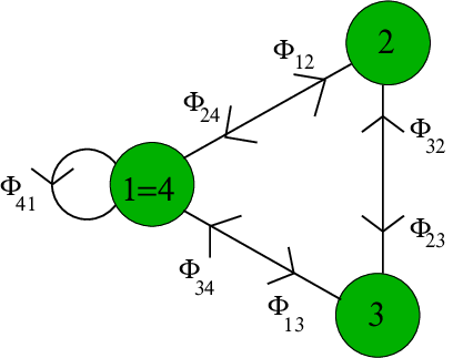
We thus start by spelling out the field content of the $\mathbb{C}^{2}/\mathbb{Z}_{2}$ quiver gauge theory, including the instanton sector. It is simply obtained recalling that the orbifold action acts as $g:(z_{1},z_{2},z_{3})\rightarrow(z_{1},-z_{2},-z_{3})$ and that its representation on the Chan-Paton indices is given by $\gamma(g)\equiv\sigma_{3}$. As reviewed in the previous section we get a block-diagonal gauge field (each block can be as usual considered a $N_{i}\times N_{j}$ matrix in general) and the matter fields are

$$\Phi^{1}=\begin{pmatrix}\Phi_{11}&\\ &\Phi_{22}\end{pmatrix},\quad\Phi^{2}=\begin{pmatrix}&\Phi_{12}\\ \Phi_{21}&\end{pmatrix},\quad\Phi^{3}=\begin{pmatrix}&\Phi^{\prime}_{12}\\ \Phi^{\prime}_{21}&\end{pmatrix}~,$$

(8)

see the quiver diagram in Figure 1.

The superpotential is given by (Note, from here on we will omit writing the trace explicitly):

$$W_{\mathbb{Z}_{2}}=\Phi^{\prime}_{21}\Phi_{11}\Phi_{12}-\Phi_{21}\Phi_{11}\Phi^{\prime}_{12}+\Phi^{\prime}_{12}\Phi_{22}\Phi_{21}-\Phi_{12}\Phi_{22}\Phi^{\prime}_{21}$$

(9)

just by replacing (8) in the ${\cal N}=4$ expression (3).

In the instanton sector, we first consider the bosonic neutral modes, which are generally matrices constituted by $k_{i}\times k_{j}$ matrix blocks, where $k_{i}$ can be considered as the instanton number in the gauge group of each node. Then the $a_{\mu}$ are block diagonal as the $A_{\mu}$ gauge fields, and the $s^{i}$ have the same form as the $\Phi^{i}$.

The projection of the fermionic neutral modes has also been reviewed in the previous section and turns out to be

	$\displaystyle M^{1}=\begin{pmatrix}M_{11}&\\ &M_{22}\end{pmatrix},\quad M^{2}=\begin{pmatrix}&M_{12}\\ M_{21}&\end{pmatrix},$
	$\displaystyle M^{3}=\begin{pmatrix}&M^{\prime}_{12}\\ M^{\prime}_{21}&\end{pmatrix},\quad M^{4}=\begin{pmatrix}M^{\prime}_{11}&\\ &M^{\prime}_{22}\end{pmatrix}$		(10)

where we have suppressed the spinor index $\alpha$. The structure of the $\lambda^{\dot{\alpha}}_{A}$ zero modes is exactly the same as above.

For the charged instanton zero modes, we can decompose the matrices into $k_{i}\times N_{j}$ and $N_{i}\times k_{j}$ blocks. The bosonic modes $\omega_{\dot{\alpha}}$ and $\bar{\omega}_{\dot{\alpha}}$ are block diagonal, while the fermionic modes $\mu^{A}$ and $\bar{\mu}^{A}$ have the same form as in (10) above. From now on we will denote all the modes by indices relating them to the relevant instanton and/or gauge nodes, see Figure 2.

The complete action for the zero modes above, and their coupling to the matter fields, is simply given by plugging back the above definitions into the ${\cal N}=4$ action given in the previous section.

We can now perform the higgsing, which corresponds to resolving the $\mathbb{C}\times(\mathbb{C}^{2}/\mathbb{Z}_{2})$ singularity to (locally) $\mathbb{C}^{3}$. In the quiver, this is achieved by giving a VEV proportional to the identity to a bifundamental field:

$$\Phi^{\prime}_{21}=m.$$

(11)

Of course, this requires the two gauge groups to have the same rank $N_{1}=N_{2}\equiv N$. Moreover, giving a VEV to a single field is consistent only if we turn on (opposite) FI terms for the diagonal $U(1)$ factors of both nodes, $\xi_{2}=-\xi_{1}=|m|^{2}$.

From the superpotential (9), we see that such a VEV gives a mass to the fields $\Phi_{12}$ and $\Phi_{11}-\Phi_{22}$, which can then be integrated out. The F-term for $\Phi_{12}$ sets $\Phi_{11}=\Phi_{22}$ exactly, so that we are left with the 3 matter fields $\Phi_{11}$, $\Phi_{21}$, $\Phi^{\prime}_{12}$ and 2 terms in the superpotential which reproduce the $\mathcal{N}=4$ superpotential (3), see Figure 3.

We can now start to consider the effect of the VEV (11) on the instanton zero modes, see Figure 4.

First of all, we consider the coupling of the matter fields to the bosonic charged zero modes $\omega_{\dot{\alpha}}$ and $\bar{\omega}_{\dot{\alpha}}$. The relevant piece of the instanton action, if we do not include the neutral $s$ fields, reads:

$$S_{2}\supset\frac{1}{2}\Big(\bar{\omega}_{11}\Phi^{\prime\dagger}_{12}\Phi^{\prime}_{21}\omega_{11}+\bar{\omega}_{22}\Phi^{\prime}_{21}\Phi^{\prime\dagger}_{12}\omega_{22}\Big)=\frac{1}{2}|m|^{2}(\bar{\omega}_{11}\omega_{11}+\bar{\omega}_{22}\omega_{22})~,$$

(12)

where we have suppressed the $\dot{\alpha}$ indices and denoted $(\Phi_{ij})^{\dagger}=\Phi^{\dagger}_{ji}$. We see that, as it stands above, a single VEV would actually give a mass and lift all the charged bosonic zero modes. This is clearly not what we expect, since of course there should be one pair of charged bosonic zero modes in the ${\cal N}=4$ theory we obtain after higgsing.

In order to recover this result, we see that we also have to consider the coupling to the neutral bosonic zero modes $s^{\prime}_{21}$:

$$S_{2}\supset\frac{1}{2}\Big(\bar{\omega}_{11}\Phi^{\prime\dagger}_{12}+s^{\prime\dagger}_{12}\bar{\omega}_{22}\Big)\Big(\Phi^{\prime}_{21}\omega_{11}+\omega_{22}s^{\prime}_{21}\Big)+\frac{1}{2}\Big(\bar{\omega}_{22}\Phi^{\prime}_{21}+s^{\prime}_{21}\bar{\omega}_{11}\Big)\Big(\Phi^{\prime\dagger}_{12}\omega_{22}+\omega_{11}s^{\prime\dagger}_{12}\Big).$$

(13)

It is clear that if we give a VEV

$$s^{\prime}_{21}=-m$$

(14)

then the above action becomes a mass term for only one linear combination of the zero modes

$$S_{2}\supset|m|^{2}(\bar{\omega}_{11}-\bar{\omega}_{22})(\omega_{11}-\omega_{22}).$$

(15)

That the neutral bosonic zero mode acquires a VEV such as (14) can be understood as follows. Recall that in order to give a VEV to the matter field, we have to turn on FI terms. Those are actually associated to turning on a background value for a closed string (twisted) modulus. As the disk amplitudes with spacefilling or euclidean boundaries are very much alike, we expect that a FI term will also appear in the D-term-like piece of the action for the $s_{i}$ as given in (7). Consequently, the action will be mininized by giving a VEV to the bosonic zero mode in (14). Note also that the F-term like piece of (6) will in turn produce mass terms that lift the zero modes $s_{12}$ and $s_{11}-s_{22}$, exactly in the same way as it happens in the matter sector.⁵⁵ 5 We see that in order for the latter zero modes to be consistently lifted, the ADHM scaling limit that suppresses (6) has to be performed after the VEV, or FI parameter, is turned on. In other words, the VEV will have to eventually scale in the ADHM limit in such a way that the masses for the zero modes that we have integrated out do not vanish.

Taking now $\bar{\omega}_{11}=\bar{\omega}_{22}$, $\omega_{11}=\omega_{22}$, $s_{11}=s_{22}$ and $s_{12}=0$ (the latter equality can be seen as a consequence of the scaling limit, see the discussion later on), we see that the action coupling the bosonic zero modes and the matter fields is exactly the one for the ${\cal N}=4$ theory, as in the first line of (3), after we make the identifications $\Phi_{11}\equiv\Phi_{22}=\frac{1}{\sqrt{2}}\Phi^{1}$, $\Phi_{21}=\Phi^{2}$, $\Phi^{\prime}_{12}=\Phi^{3}$ and similarly for the $s^{i}$. (The factors of $\sqrt{2}$ are necessary in order to keep all the fields canonically normalized.)

We now turn to consider the fermionic charged zero modes $\bar{\mu}$ and $\mu$. Inserting the VEVs (11) and (14) in (3), we obtain the following “mass” terms: (dropping an overall normalization factor)

$$S_{2}\supset m^{*}\bar{\mu}^{\prime}_{21}(\mu^{\prime}_{11}-\mu^{\prime}_{22})+m^{*}(\bar{\mu}^{\prime}_{11}-\bar{\mu}^{\prime}_{22})\mu^{\prime}_{21}+m\bar{\mu}_{12}(\mu_{11}-\mu_{22})+m(\bar{\mu}_{11}-\bar{\mu}_{22})\mu_{12}~.$$

(16)

In order to integrate out these 8 zero modes, one should perform a Gaussian integral. This involves a non-trivial determinant, since there are other terms in (3), involving the above fermionic zero modes coupling to matter fields and neutral bosonic zero modes. However, one easily realizes that in order to match the result of this integration with the ${\cal N}=4$ result, one has to set to zero (i.e. scale away) all terms that have a prefactor which is at least $1/|m|^{2}$. This is what we will indeed do here and in the following, but note that we are nevertheless allowing for the possibility of keeping terms which go as some power of $1/m$ or of $1/m^{*}$, i.e. are holomorphic or anti-holomorphic in $m$. The reason why we want to keep them will be clear in the next section, where we perform two or more consecutive higgsings. Why “holomorphic” terms do not scale away while non-holomorphic ones do cannot be rigorously justified in the present set up, but is presumably related to the fact that the former are protected while the latter receive large corrections during the non-trivial RG flow that the theory undergoes from its classical description discussed here and its IR effective dynamics.

As we are interested only in the corrections proportional to $1/m$ or $1/m^{*}$, we can integrate out independently the two sets of modes, by setting in turn $1/m=0$ and $1/m^{*}=0$. Doing this, it turns out that everything works in the present case as if we could set all the “massive” zero modes to zero, hence imposing $\mu_{11}=\mu_{22}$ and $\mu^{\prime}_{11}=\mu^{\prime}_{22}$ exactly, and similarly for the barred ones.

Performing the identifications as before, together with $\mu_{11}=\frac{1}{\sqrt{2}}\mu^{1}$, $\mu_{21}=\mu^{2}$, $\mu^{\prime}_{12}=\mu^{3}$, $\mu^{\prime}_{11}=\frac{1}{\sqrt{2}}\mu^{4}$ and similarly for $\bar{\mu}^{A}$, we obtain exactly the couplings in the second line of (3), up to a global prefactor of $\frac{1}{\sqrt{2}}$ which can be reabsorbed by performing a further overall rescaling.

We are left to discuss the bosonic neutral zero modes $a_{\mu}$ and the fermionic ones $M^{A}$ and $\lambda_{A}$. All the relevant components of these zero modes are lifted by the VEV of the zero mode $s^{\prime}_{21}$ exactly in the same way as the VEV for $\Phi^{\prime}_{21}$ lifts the gauge fields and the gaugini superpartners of the fields which become massive. For instance, the components $M_{11}-M_{22}$, $M^{\prime}_{11}-M^{\prime}_{22}$, $M^{\prime}_{21}$ and $M_{12}$ will be lifted through the couplings in the last two terms in the first line of (4). Similarly, the components $\lambda_{11}-\lambda_{22}$, $\lambda^{\prime}_{11}-\lambda^{\prime}_{22}$, $\lambda^{\prime}_{12}$ and $\lambda_{21}$ will get a mass through the couplings in the last two terms in the first line of (6). Note that this too implies that the ADHM limit has to be taken in such a way that these mass terms are not washed away. Eventually, the first term in the first line of (4) gives a mass to the combination $a_{\mu 11}-a_{\mu 22}$, leaving the center-of-mass bosonic zero modes as the ones relevant for the instantons in the $\mathcal{N}=4$ theory.⁶⁶ 6 The auxiliary terms $D^{a}$ are already massive. The ones which are related to $a_{\mu}$ zero modes that have become massive can be integrated out trivially by setting them to zero.

As a last routine check, one can reexpress the last two lines of (4) in terms of the zero modes that have been kept and recover the $\mathcal{N}=4$ expression.

We have thus addressed in this section all the subtleties related to the higgsing procedure in the instanton sector which are already present when one is going from one orbifold singularity to another. In the following section we can thus address the additional features that appear when one exits the realm of orbifold singularities.

We now address the first instance of higgsing to a non-orbifold toric geometry, where it is less direct to compute the spectrum and action by perturbative methods.

There is a major difference between orbifold and non-orbifold (toric) quivers, in the sense that orbifold quivers are conformal at the classical and perturbative level, while the non-orbifold quivers are typically non-conformal classically (there are terms higher than cubic in the superpotential) but possess a non-trivial superconformal fixed point at finite coupling. Hence non orbifold quivers are defined by the classical field content and superpotential up to this RG flow to the IR fixed point. We conjecture here that the structure of the instanton moduli does not change along this flow. That this is a consistent thing to do is checked by higgsing back to some other orbifold quiver, and recovering the spectrum and couplings computed in perturbation theory.

We will start from the $\mathbb{C}^{3}/\mathbb{Z}_{2}\times\mathbb{Z}_{2}$ four node quiver, and higgs it to the Suspended Pinch Point (SPP) three node quiver. Then we will further higgs the latter to the previously discussed $\mathbb{C}^{2}/\mathbb{Z}_{2}$ two node quiver, as a consistency check. We will also higgs the SPP to the Conifold quiver, to gain confidence in the structure of the moduli action in the non-orbifold case. Consistency is again checked by further higgsing the Conifold to recover the ${\cal N}=4$ theory.

Note that the only non generic feature of the quiver gauge theories discussed in this section is that they are non-chiral. We will address the more general chiral theories later on, but we anticipate that there will be no additional features as far as the construction of the instanton action is concerned.

We begin by concisely reviewing the structure of the $\mathbb{C}^{3}/\mathbb{Z}_{2}\times\mathbb{Z}_{2}$ quiver gauge theory and of its instanton zero modes, see [49, 66]. (This orbifold has been recently investigated from the point of view of string phenomenology in [67]). As in [21], the orbifold is taken as $g_{1}:(z_{1},z_{2},z_{3})\rightarrow(z_{1},-z_{2},-z_{3})$ and $g_{2}:(z_{1},z_{2},z_{3})\rightarrow(-z_{1},z_{2},-z_{3})$, with the representation on the Chan-Paton indices being $\gamma(g_{1})=\sigma_{3}\otimes\mathbf{1}$ and $\gamma(g_{2})=\mathbf{1}\otimes\sigma_{3}$. Then, the gauge fields and the 3 matter fields are given by

	$\displaystyle A^{\mu}=\begin{pmatrix}A^{\mu}_{11}&0&0&0\cr 0&A^{\mu}_{22}&0&0\cr 0&0&A^{\mu}_{33}&0\cr 0&0&0&A^{\mu}_{44}\cr\end{pmatrix},$		$\displaystyle\Phi^{1}=\begin{pmatrix}0&\Phi_{12}&0&0\cr\Phi_{21}&0&0&0\cr 0&0&0&\Phi_{34}\cr 0&0&\Phi_{43}&0\cr\end{pmatrix},$
	$\displaystyle\Phi^{2}=\begin{pmatrix}0&0&\Phi_{13}&0\cr 0&0&0&\Phi_{24}\cr\Phi_{31}&0&0&0\cr 0&\Phi_{42}&0&0\cr\end{pmatrix},$		$\displaystyle\Phi^{3}=\begin{pmatrix}0&0&0&\Phi_{14}\cr 0&0&\Phi_{23}&0\cr 0&\Phi_{32}&0&0\cr\Phi_{41}&0&0&0\cr\end{pmatrix}~.$		(17)

As already discussed in full generality, in the instanton sector $s^{i},M^{i},\lambda_{i},\mu^{i},\bar{\mu}^{i}$ acquire the same structure as $\Phi^{i}$, whereas $a_{\mu},D_{c},\omega,\bar{\omega},M^{4},\lambda_{4},\mu^{4},\bar{\mu}^{4}$ are all block diagonal as $A_{\mu}$.

The superpotential for the $\mathbb{C}^{3}/\mathbb{Z}_{2}\times\mathbb{Z}_{2}$ quiver is simply

	$\displaystyle W_{\mathbb{Z}_{2}\times\mathbb{Z}_{2}}$	$\displaystyle=$	$\displaystyle\Phi_{31}\Phi_{12}\Phi_{23}-\Phi_{31}\Phi_{14}\Phi_{43}-\Phi_{13}\Phi_{32}\Phi_{21}+\Phi_{13}\Phi_{34}\Phi_{41}$		(18)
			$\displaystyle+\Phi_{42}\Phi_{21}\Phi_{14}-\Phi_{42}\Phi_{23}\Phi_{34}-\Phi_{24}\Phi_{41}\Phi_{12}+\Phi_{24}\Phi_{43}\Phi_{32}~.$

We can now see what happens if we give a VEV such as

$$\Phi_{14}=m.$$

(19)

This requires the condition $N_{1}=N_{4}=N$ and breaks the two gauge groups corresponding to nodes 1 and 4 to the diagonal subgroup,

$$SU(N)_{1}\times SU(N)_{4}\to SU(N)_{(14)}~.$$

(20)

The chiral superfield $\Phi_{41}$ will thereby transform in the adjoint representation of $SU(N)_{(14)}$. We immediately see that the fields $\Phi_{31}$, $\Phi_{43}$, $\Phi_{42}$ and $\Phi_{21}$ become massive. One should integrate them out through their F-flatness equations, which read:

	$\displaystyle\Phi_{31}=\frac{1}{m}\Phi_{32}\Phi_{24},$		$\displaystyle\Phi_{43}=\frac{1}{m}\Phi_{12}\Phi_{23},$
	$\displaystyle\Phi_{42}=\frac{1}{m}\Phi_{13}\Phi_{32},$		$\displaystyle\Phi_{21}=\frac{1}{m}\Phi_{23}\Phi_{34}~.$		(21)

Inserting these values back into (18) gives us the SPP superpotential,

$$W_{SPP}=\frac{1}{m}\Phi_{24}\Phi_{12}\Phi_{23}\Phi_{32}-\frac{1}{m}\Phi_{13}\Phi_{32}\Phi_{23}\Phi_{34}+\Phi_{13}\Phi_{34}\Phi_{41}-\Phi_{24}\Phi_{41}\Phi_{12}$$

(22)

where all the remaining fields (except for $\Phi_{41}$) transform in bifundamental representations of two of the factors in the gauge group $SU(N)_{(14)}\times SU(N_{2})\times SU(N_{3})$, see Figure 5.

We can continue with this procedure and obtain the quiver gauge theory for a $\mathbb{Z}_{2}$ orbifold if we start from the SPP theory and give an additional VEV to the chiral superfield $\Phi_{32}$,

$$\Phi_{32}=m~.$$

(23)

This means that we have the condition $N_{3}=N_{2}=M$ and that we “pinch” the two gauge groups corresponding to nodes 2 and 3 together,

$$SU(M)_{2}\times SU(M)_{3}\to SU(M)_{(23)}~.$$

(24)

As before, the chiral superfield $\Phi_{23}$ will now transform in the adjoint representation of SU$(M)_{(23)}$. We see from (22) that (23) does not induce any new mass terms, but gives us the $\mathbb{Z}_{2}$ superpotential, (same as (9) upon relabeling)

$$W_{\mathbb{Z}_{2}}=\Phi_{24}\Phi_{12}\Phi_{23}-\Phi_{13}\Phi_{23}\Phi_{34}+\Phi_{13}\Phi_{34}\Phi_{41}-\Phi_{24}\Phi_{41}\Phi_{12}$$

(25)

where $\Phi_{12}$, $\Phi_{13}$ are in the ($\square$,$\overline{\square}$) of the gauge group $SU(N)_{(14)}\times SU(M)_{(23)}$, while $\Phi_{24}$, $\Phi_{34}$ are in the ($\overline{\square}$,$\square$) and $\Phi_{41}$, $\Phi_{23}$ are in the adjoint of the respective gauge groups, see Figure 6.

To get the conifold gauge theory, we start again from the SPP theory but now we instead give a VEV to the chiral superfield $\Phi_{34}$,

$$\Phi_{34}=m.$$

(26)

This implies the condition $N_{1}=N_{4}=N_{3}=N$, such that the three gauge groups corresponding to nodes 1, 3 and 4 now become

$$SU(N)_{1}\times SU(N)_{3}\times SU(N)_{4}\to SU(N)_{(134)}~.$$

(27)

We see from (22) that (26) induces a mass term for the bifundamental chiral superfield $\Phi_{13}$ and the adjoint field $\Phi_{41}$. Hence, we solve for these fields and get the following expressions,

$$\Phi_{13}=\frac{1}{m}\Phi_{12}\Phi_{24},\qquad\Phi_{41}=\frac{1}{m}\Phi_{32}\Phi_{23}~.$$

(28)

Inserting (26) and (28) into (22) yields the superpotential for the conifold,

$\displaystyle W_{con}$

$\displaystyle=$

$\displaystyle\frac{1}{m}\Phi_{12}\Phi_{23}\Phi_{32}\Phi_{24}-\frac{1}{m}\Phi_{12}\Phi_{24}\Phi_{32}\Phi_{23}$

(29)

where $\Phi_{12}$, $\Phi_{32}$ are in the ($\square$,$\overline{\square}$) of the gauge group $SU(N)_{(134)}\times SU(N_{2})$, $\Phi_{24}$, $\Phi_{23}$ are in the ($\overline{\square}$,$\square$) and there are no more adjoint fields, see Figure 7.

From here, giving a VEV to, say, $\Phi_{24}=m$, leads straightforwardly to the $\mathcal{N}=4$ theory and its cubic superpotential, see Figure 8.

All the above is of course standard, but we will now see how this higgsing pattern extends to the instanton sector.

Let us consider our first non-trivial step out of the orbifold realm. As reviewed in the previous section, in the absence of any other field acquiring a VEV, the effect that $\Phi_{14}=m$ would produce is to give a mass to both pairs of bosonic charged moduli $\omega_{11}$, $\bar{\omega}_{11}$ and $\omega_{44}$, $\bar{\omega}_{44}$. We know that in order to lift only one combination of these two pairs of zero modes, we need to turn on the VEV

$$s_{14}=-m.$$

(30)

We will then have

	$\displaystyle S_{2}$	$\displaystyle\supset$	$\displaystyle\frac{1}{2}\Big(\bar{\omega}_{11}\Phi_{14}+s_{14}\bar{\omega}_{44}\Big)\Big(\Phi^{\dagger}_{41}\omega_{11}+\omega_{44}s^{\dagger}_{41}\Big)+\frac{1}{2}\Big(\bar{\omega}_{44}\Phi^{\dagger}_{41}+s^{\dagger}_{41}\bar{\omega}_{11}\Big)\Big(\Phi_{14}\omega_{44}+\omega_{11}s_{14}\Big)$		(31)
		$\displaystyle=$	$\displaystyle|m|^{2}(\bar{\omega}_{11}-\bar{\omega}_{44})(\omega_{11}-\omega_{44}).$

We thus see that we can set $\bar{\omega}_{11}=\bar{\omega}_{44}$ and $\omega_{11}=\omega_{44}$. The action coupling the bosonic charged zero modes to the matter fields and to the neutral bosonic zero modes is obtained as follows. We see that if we replace the fields that we have integrated out (21) by their values in the action for the orbifold zero modes, we would get a series of terms which are quartic in the matter fields and have a $\frac{1}{|m|^{2}}$ prefactor. Similarly, we know that because of the F-terms in (6) the zero modes $s_{31}$, $s_{43}$, $s_{42}$ and $s_{21}$ will be integrated out, with expressions such as $s_{31}=-\frac{1}{m}s_{32}s_{24}$. Hence there would also be terms quartic in the $s^{i}$, and terms such as $\bar{\omega}\Phi\Phi\omega s^{\dagger}s^{\dagger}$. However, all of these terms have the same $\frac{1}{|m|^{2}}$ prefactor, and we will assume, based on consistency with further higgsing, that these terms are suppressed due to the RG flow that essentially decouples the massive modes (both in the matter and in the instanton sectors).

Hence, we can write the following action:

	$\displaystyle S^{\omega}_{SPP}$	$\displaystyle=$	$\displaystyle\big(\bar{\omega}_{11}\Phi_{12}+s_{12}\bar{\omega}_{22}\big)\big(\Phi^{\dagger}_{21}\omega_{11}+\omega_{22}s^{\dagger}_{21}\big)+\big(\bar{\omega}_{22}\Phi^{\dagger}_{21}+s^{\dagger}_{21}\bar{\omega}_{11}\big)\big(\Phi_{12}\omega_{22}+\omega_{11}s_{12}\big)$
		$\displaystyle+$	$\displaystyle\big(\bar{\omega}_{11}\Phi_{13}+s_{13}\bar{\omega}_{33}\big)\big(\Phi^{\dagger}_{31}\omega_{11}+\omega_{33}s^{\dagger}_{31}\big)+\big(\bar{\omega}_{33}\Phi^{\dagger}_{31}+s^{\dagger}_{31}\bar{\omega}_{11}\big)\big(\Phi_{13}\omega_{33}+\omega_{11}s_{13}\big)$
		$\displaystyle+$	$\displaystyle\big(\bar{\omega}_{22}\Phi_{24}+s_{24}\bar{\omega}_{11}\big)\big(\Phi^{\dagger}_{42}\omega_{22}+\omega_{11}s^{\dagger}_{42}\big)+\big(\bar{\omega}_{11}\Phi^{\dagger}_{42}+s^{\dagger}_{42}\bar{\omega}_{22}\big)\big(\Phi_{24}\omega_{11}+\omega_{22}s_{24}\big)$
		$\displaystyle+$	$\displaystyle\big(\bar{\omega}_{33}\Phi_{34}+s_{34}\bar{\omega}_{11}\big)\big(\Phi^{\dagger}_{43}\omega_{33}+\omega_{11}s^{\dagger}_{43}\big)+\big(\bar{\omega}_{11}\Phi^{\dagger}_{43}+s^{\dagger}_{43}\bar{\omega}_{33}\big)\big(\Phi_{34}\omega_{11}+\omega_{33}s_{34}\big)$
		$\displaystyle+$	$\displaystyle\big(\bar{\omega}_{22}\Phi_{23}+s_{23}\bar{\omega}_{33}\big)\big(\Phi^{\dagger}_{32}\omega_{22}+\omega_{33}s^{\dagger}_{32}\big)+\big(\bar{\omega}_{33}\Phi^{\dagger}_{32}+s^{\dagger}_{32}\bar{\omega}_{22}\big)\big(\Phi_{23}\omega_{33}+\omega_{22}s_{23}\big)$
		$\displaystyle+$	$\displaystyle\big(\bar{\omega}_{33}\Phi_{32}+s_{32}\bar{\omega}_{22}\big)\big(\Phi^{\dagger}_{23}\omega_{33}+\omega_{22}s^{\dagger}_{23}\big)+\big(\bar{\omega}_{22}\Phi^{\dagger}_{23}+s^{\dagger}_{23}\bar{\omega}_{33}\big)\big(\Phi_{32}\omega_{22}+\omega_{33}s_{32}\big)$
		$\displaystyle+$	$\displaystyle\big(\bar{\omega}_{11}\Phi_{41}+s_{41}\bar{\omega}_{11}\big)\big(\Phi^{\dagger}_{14}\omega_{11}+\omega_{11}s^{\dagger}_{14}\big)+\big(\bar{\omega}_{11}\Phi^{\dagger}_{14}+s^{\dagger}_{14}\bar{\omega}_{11}\big)\big(\Phi_{41}\omega_{11}+\omega_{11}s_{41}\big)$

In presenting the above actions and in all the following ones we find ourself facing a notational dilemma. The higgsing procedure removes some of the nodes making some of the indices obsolete. One could relabel the indices at every step, for instance in the case under consideration letting $4\to 1$ everywhere. The advantage of doing this is that the instanton action for each model looks more intelligible but the disadvantage is that this relabeling makes it difficult to follow the chain of higgsings from one model to another. We choose not to relabel the fields at this stage and ask the reader to keep track of which nodes are identified. We will however still set $\omega_{44}=\omega_{11}$ etc. because these are two previously distinct moduli fields that are now identified by the higgsing procedure.

As we turn to consider the charged fermionic zero modes, we see that the VEVs for $\Phi_{14}$ and $s_{14}$ yield the following mass terms:

$$S_{2}\supset m^{*}\big[\bar{\mu}_{14}(\mu_{11}-\mu_{44})+(\bar{\mu}_{11}-\bar{\mu}_{44})\mu_{14}\big]+m\big(\bar{\mu}_{21}\mu_{42}+\bar{\mu}_{42}\mu_{21}-\bar{\mu}_{31}\mu_{43}-\bar{\mu}_{43}\mu_{31}\big)$$

(33)

As in the previous section, the complete action coupling $\mu,\bar{\mu}$ to $\Phi$ and $s$ will contain other terms involving the above massive zero modes. These would lead to very complicated expressions mixing the holomorphic/anti-holomorphic components. Again, consistency is obtained if and only if we decouple all terms with a $\frac{1}{|m|^{2}}$ prefactor, thus preserving the holomorphic/anti-holomorphic serparation. The remaining terms are computed by setting in turn $\frac{1}{m}=0$ and $\frac{1}{m^{*}}=0$ and reinstating the finite value of $m$ in the end, after the integration.

If we set $\frac{1}{m}=0$, and thus set exactly to zero all the modes which have a mass $m$, we observe that no couplings remain which involve $\mu_{14}$ or $\bar{\mu}_{14}$. Hence, $\mu_{11}-\mu_{44}$ and $\bar{\mu}_{11}-\bar{\mu}_{44}$ act like Lagrange multipliers and integrating out the modes with a mass $m^{*}$ is equivalent to setting to zero all terms in which they appear.

On the other hand setting $\frac{1}{m^{*}}=0$, we set exactly to zero the modes with mass $m^{*}$, but this still leaves terms which mix the remaining massless modes with the modes of mass $m$. Hence integrating out the latter yields non trivial expressions. Yet it is remarkable that these expressions only contain holomorphic dependence on the fields $\Phi$ and $s$.

It is easy to see that because of the structure of the terms involving $\Phi^{\dagger}$ and $s^{\dagger}$, and due to the previous remarks, no terms linear in $\frac{1}{m^{*}}$ will be generated at all. Hence, the part of the action coupling the fermionic charged zero modes to the anti-holomorphic fields will remain cubic:

	$\displaystyle S_{SPP}^{\overline{\mathrm{holo}}}$	$\displaystyle=$	$\displaystyle\big(\bar{\mu}_{41}\Phi^{\dagger}_{14}+\bar{\mu}_{12}\Phi^{\dagger}_{21}+\bar{\mu}_{13}\Phi^{\dagger}_{31}\big)\mu_{11}+\big(\bar{\mu}_{23}\Phi^{\dagger}_{32}+\bar{\mu}_{24}\Phi^{\dagger}_{42}\big)\mu_{22}$		(34)
			$\displaystyle+\big(\bar{\mu}_{32}\Phi^{\dagger}_{23}+\bar{\mu}_{34}\Phi^{\dagger}_{43}\big)\mu_{33}+\big(s^{\dagger}_{14}\bar{\mu}_{41}+s^{\dagger}_{42}\bar{\mu}_{24}+s^{\dagger}_{43}\bar{\mu}_{34}\big)\mu_{11}$
			$\displaystyle+\big(s^{\dagger}_{21}\bar{\mu}_{12}+s^{\dagger}_{23}\bar{\mu}_{32}\big)\mu_{22}+\big(s^{\dagger}_{31}\bar{\mu}_{13}+s^{\dagger}_{32}\bar{\mu}_{23}\big)\mu_{33}$
			$\displaystyle-\bar{\mu}_{11}\big(\Phi^{\dagger}_{14}\mu_{41}+\Phi^{\dagger}_{42}\mu_{24}+\Phi^{\dagger}_{43}\mu_{34}\big)-\bar{\mu}_{22}\big(\Phi^{\dagger}_{21}\mu_{12}+\Phi^{\dagger}_{23}\mu_{32}\big)$
			$\displaystyle-\bar{\mu}_{33}\big(\Phi^{\dagger}_{31}\mu_{13}+\Phi^{\dagger}_{32}\mu_{23}\big)-\bar{\mu}_{11}\big(\mu_{41}s^{\dagger}_{14}+\mu_{12}s^{\dagger}_{21}+\mu_{13}s^{\dagger}_{31}\big)$
			$\displaystyle-\bar{\mu}_{22}\big(\mu_{24}s^{\dagger}_{42}+\mu_{23}s^{\dagger}_{32}\big)-\bar{\mu}_{33}\big(\mu_{34}s^{\dagger}_{43}+\mu_{32}s^{\dagger}_{23}\big)$

The expressions for the charged fermionic zero modes of mass $m$ which have been integrated out are

	$\displaystyle\mu_{31}=\frac{1}{m}\big(\Phi_{32}\mu_{24}-\mu_{32}s_{24}\big),$		$\displaystyle\bar{\mu}_{31}=\frac{1}{m}\big(\bar{\mu}_{32}\Phi_{24}-s_{32}\bar{\mu}_{24}\big),$
	$\displaystyle\mu_{43}=\frac{1}{m}\big(\Phi_{12}\mu_{23}-\mu_{12}s_{23}\big),$		$\displaystyle\bar{\mu}_{43}=\frac{1}{m}\big(\bar{\mu}_{12}\Phi_{23}-s_{12}\bar{\mu}_{23}\big),$
	$\displaystyle\mu_{42}=\frac{1}{m}\big(\Phi_{13}\mu_{32}-\mu_{13}s_{32}\big),$		$\displaystyle\bar{\mu}_{42}=\frac{1}{m}\big(\bar{\mu}_{13}\Phi_{32}-s_{13}\bar{\mu}_{32}\big),$
	$\displaystyle\mu_{21}=\frac{1}{m}\big(\Phi_{23}\mu_{34}-\mu_{23}s_{34}\big),$		$\displaystyle\bar{\mu}_{21}=\frac{1}{m}\big(\bar{\mu}_{23}\Phi_{34}-s_{23}\bar{\mu}_{34}\big).$		(35)

One can actually replace all the terms where the above massive modes appear by substituting the above expressions in the mass terms of the second line of (33). This will clearly lead to terms like $\bar{\mu}\Phi\Phi\mu$, $\bar{\mu}\mu ss$ and $\bar{\mu}\Phi\mu s$. Other terms like $\bar{\mu}\Phi\Phi\mu$ and $\bar{\mu}\mu ss$ are generated when replacing the expressions such as (21) for the $\Phi$ and $s$ modes that are also integrated out. All in all, we arrive at the following expression for the holomorphic couplings of the fermionic charged zero modes:

	$\displaystyle S_{SPP}^{\mathrm{holo}}$	$\displaystyle=$	$\displaystyle\frac{1}{m}(\bar{\mu}_{24}\mu_{12}s_{23}s_{32}-\bar{\mu}_{24}\Phi_{12}\mu_{23}s_{32}+\bar{\mu}_{24}\Phi_{12}\Phi_{23}\mu_{32}+\bar{\mu}_{12}\mu_{23}s_{32}s_{24}$		(36)
			$\displaystyle-\bar{\mu}_{12}\Phi_{23}\mu_{32}s_{24}+\bar{\mu}_{12}\Phi_{23}\Phi_{32}\mu_{24}+\bar{\mu}_{23}\mu_{32}s_{24}s_{12}-\bar{\mu}_{23}\Phi_{32}\mu_{24}s_{12}$
			$\displaystyle+\bar{\mu}_{23}\Phi_{32}\Phi_{24}\mu_{12}+\bar{\mu}_{32}\mu_{24}s_{12}s_{23}-\bar{\mu}_{32}\Phi_{24}\mu_{12}s_{23}+\bar{\mu}_{32}\Phi_{24}\Phi_{12}\mu_{23})$
			$\displaystyle-\frac{1}{m}(\bar{\mu}_{13}\mu_{32}s_{23}s_{34}-\bar{\mu}_{13}\Phi_{32}\mu_{23}s_{34}+\bar{\mu}_{13}\Phi_{32}\Phi_{23}\mu_{34}+\bar{\mu}_{32}\mu_{23}s_{34}s_{13}$
			$\displaystyle-\bar{\mu}_{32}\Phi_{23}\mu_{34}s_{13}+\bar{\mu}_{32}\Phi_{23}\Phi_{34}\mu_{13}+\bar{\mu}_{23}\mu_{34}s_{13}s_{32}-\bar{\mu}_{23}\Phi_{34}\mu_{13}s_{32}$
			$\displaystyle+\bar{\mu}_{23}\Phi_{34}\Phi_{13}\mu_{32}+\bar{\mu}_{34}\mu_{13}s_{32}s_{23}-\bar{\mu}_{34}\Phi_{13}\mu_{32}s_{23}+\bar{\mu}_{34}\Phi_{13}\Phi_{32}\mu_{23})$
			$\displaystyle-\bar{\mu}_{13}\mu_{34}s_{41}+\bar{\mu}_{13}\Phi_{34}\mu_{41}-\bar{\mu}_{34}\mu_{41}s_{13}+\bar{\mu}_{34}\Phi_{41}\mu_{13}$
			$\displaystyle-\bar{\mu}_{41}\mu_{13}s_{34}+\bar{\mu}_{41}\Phi_{13}\mu_{34}+\bar{\mu}_{24}\mu_{41}s_{12}-\bar{\mu}_{24}\Phi_{41}\mu_{12}$
			$\displaystyle+\bar{\mu}_{41}\mu_{12}s_{24}-\bar{\mu}_{41}\Phi_{12}\mu_{24}+\bar{\mu}_{12}\mu_{24}s_{41}-\bar{\mu}_{12}\Phi_{24}\mu_{41}$

References

- [1] A. A. Belavin, A. M. Polyakov, A. S. Shvarts and Yu. S. Tyupkin, Phys. Lett. B 59 (1975) 85.
- [2] G. ’t Hooft, Phys. Rev. D 14, 3432 (1976) [Erratum-ibid. D 18, 2199 (1978)].
- [3] J. Polchinski, Phys. Rev. Lett. 75 (1995) 4724 [arXiv:hep-th/9510017].
- [4] E. Witten, Nucl. Phys. B 460 (1996) 541 [arXiv:hep-th/9511030].
- [5] M. R. Douglas, arXiv:hep-th/9512077.
- [6] E. Witten, Nucl. Phys. B 474, 343 (1996) [arXiv:hep-th/9604030].
- [7] O. J. Ganor, Nucl. Phys. B 499, 55 (1997) [arXiv:hep-th/9612077].
- [8] M. B. Green and M. Gutperle, JHEP 0002 (2000) 014 [arXiv:hep-th/0002011].
- [9] M. Billo, M. Frau, I. Pesando, F. Fucito, A. Lerda and A. Liccardo, JHEP 0302 (2003) 045 [arXiv:hep-th/0211250].
- [10] M. Dine, N. Seiberg, X. G. Wen and E. Witten, Nucl. Phys. B 278 (1986) 769.
- [11] R. Blumenhagen, M. Cvetic and T. Weigand, Nucl. Phys. B 771 (2007) 113 [arXiv:hep-th/0609191].
- [12] M. Haack, D. Krefl, D. Lust, A. Van Proeyen and M. Zagermann, JHEP 0701 (2007) 078 [arXiv:hep-th/0609211].
- [13] L. E. Ibanez and A. M. Uranga, JHEP 0703 (2007) 052 [arXiv:hep-th/0609213].
- [14] B. Florea, S. Kachru, J. McGreevy and N. Saulina, JHEP 0705 (2007) 024 [arXiv:hep-th/0610003].
- [15] M. Buican, D. Malyshev, D. R. Morrison, H. Verlinde and M. Wijnholt, JHEP 0701 (2007) 107 [arXiv:hep-th/0610007].
- [16] S. A. Abel and M. D. Goodsell, JHEP 0710 (2007) 034 [arXiv:hep-th/0612110].
- [17] N. Akerblom, R. Blumenhagen, D. Lust, E. Plauschinn and M. Schmidt-Sommerfeld, JHEP 0704 (2007) 076 [arXiv:hep-th/0612132].
- [18] M. Bianchi and E. Kiritsis, Nucl. Phys. B 782 (2007) 26 [arXiv:hep-th/0702015].
- [19] M. Cvetic, R. Richter and T. Weigand, Phys. Rev. D 76 (2007) 086002 [arXiv:hep-th/0703028].
- [20] R. Argurio, M. Bertolini, S. Franco and S. Kachru, JHEP 0706 (2007) 017 [arXiv:hep-th/0703236].
- [21] R. Argurio, M. Bertolini, G. Ferretti, A. Lerda and C. Petersson, JHEP 0706 (2007) 067 [arXiv:0704.0262 [hep-th]].
- [22] M. Bianchi, F. Fucito and J. F. Morales, JHEP 0707 (2007) 038 [arXiv:0704.0784 [hep-th]].
- [23] L. E. Ibanez, A. N. Schellekens and A. M. Uranga, JHEP 0706 (2007) 011 [arXiv:0704.1079 [hep-th]].
- [24] N. Akerblom, R. Blumenhagen, D. Lust and M. Schmidt-Sommerfeld, Phys. Lett. B 652 (2007) 53 [arXiv:0705.2150 [hep-th]].
- [25] N. Akerblom, R. Blumenhagen, D. Lust and M. Schmidt-Sommerfeld, JHEP 0708 (2007) 044 [arXiv:0705.2366 [hep-th]].
- [26] S. Antusch, L. E. Ibanez and T. Macri, JHEP 0709 (2007) 087 [arXiv:0706.2132 [hep-ph]].
- [27] S. Franco, A. Hanany, D. Krefl, J. Park, A. M. Uranga and D. Vegh, JHEP 0709 (2007) 075 [arXiv:0707.0298 [hep-th]].
- [28] R. Blumenhagen, M. Cvetic, D. Lust, R. Richter and T. Weigand, arXiv:0707.1871 [hep-th].
- [29] M. Billo, M. Frau and A. Lerda, arXiv:0707.2298 [hep-th].
- [30] O. Aharony and S. Kachru, JHEP 0709 (2007) 060 [arXiv:0707.3126 [hep-th]].
- [31] R. Blumenhagen, M. Cvetic, R. Richter and T. Weigand, JHEP 0710 (2007) 098 [arXiv:0708.0403 [hep-th]].
- [32] O. Aharony, S. Kachru and E. Silverstein, Phys. Rev. D 76 (2007) 126009 [arXiv:0708.0493 [hep-th]].
- [33] M. Billo, M. Frau, I. Pesando, P. Di Vecchia, A. Lerda and R. Marotta, JHEP 0710 (2007) 091 [arXiv:0708.3806 [hep-th]].
- [34] M. Billo, M. Frau, I. Pesando, P. Di Vecchia, A. Lerda and R. Marotta, JHEP 0712 (2007) 051 [arXiv:0709.0245 [hep-th]].
- [35] M. Aganagic, C. Beem and S. Kachru, arXiv:0709.4277 [hep-th].
- [36] P. G. Camara, E. Dudas, T. Maillard and G. Pradisi, Nucl. Phys. B 795 (2008) 453 [arXiv:0710.3080 [hep-th]].
- [37] M. Cvetic and T. Weigand, arXiv:0711.0209 [hep-th].
- [38] L. E. Ibanez and A. M. Uranga, arXiv:0711.1316 [hep-th].
- [39] I. Garcia-Etxebarria and A. M. Uranga, JHEP 0801 (2008) 033 [arXiv:0711.1430 [hep-th]].
- [40] C. Petersson, arXiv:0711.1837 [hep-th].
- [41] R. Blumenhagen, S. Moster and E. Plauschinn, JHEP 0801 (2008) 058 [arXiv:0711.3389 [hep-th]].
- [42] M. Bianchi and J. F. Morales, arXiv:0712.1895 [hep-th].
- [43] M. Cvetic, R. Richter and T. Weigand, arXiv:0712.2845 [hep-th].
- [44] Y. Matsuo, J. Park, C. Ryou and M. Yamamoto, arXiv:0803.0798 [hep-th].
- [45] R. Blumenhagen and M. Schmidt-Sommerfeld, arXiv:0803.1562 [hep-th].
- [46] T. R. Taylor, G. Veneziano and S. Yankielowicz, Nucl. Phys. B 218 (1983) 493.
- [47] I. Affleck, M. Dine and N. Seiberg, Nucl. Phys. B 241 (1984) 493.
- [48] M. R. Douglas and G. W. Moore, arXiv:hep-th/9603167.
- [49] D. R. Morrison and M. R. Plesser, Adv. Theor. Math. Phys. 3, 1 (1999) [arXiv:hep-th/9810201].
- [50] J. Park, R. Rabadan and A. M. Uranga, Nucl. Phys. B 570 (2000) 38 [arXiv:hep-th/9907086].
- [51] C. E. Beasley and M. R. Plesser, JHEP 0112 (2001) 001 [arXiv:hep-th/0109053].
- [52] B. Feng, A. Hanany, Y. H. He and A. M. Uranga, JHEP 0112 (2001) 035 [arXiv:hep-th/0109063].
- [53] B. Feng, S. Franco, A. Hanany and Y. H. He, JHEP 0212, 076 (2002) [arXiv:hep-th/0205144].
- [54] B. Feng, A. Hanany and Y. H. He, JHEP 0108, 040 (2001) [arXiv:hep-th/0104259].
- [55] S. Franco, A. Hanany, K. D. Kennaway, D. Vegh and B. Wecht, JHEP 0601, 096 (2006) [arXiv:hep-th/0504110].
- [56] D. Martelli and J. Sparks, Commun. Math. Phys. 262 (2006) 51 [arXiv:hep-th/0411238].
- [57] S. Benvenuti, S. Franco, A. Hanany, D. Martelli and J. Sparks, JHEP 0506 (2005) 064 [arXiv:hep-th/0411264].
- [58] M. Bertolini, F. Bigazzi and A. L. Cotrone, JHEP 0412, 024 (2004) [arXiv:hep-th/0411249].
- [59] D. Berenstein, C. P. Herzog, P. Ouyang and S. Pinansky, JHEP 0509 (2005) 084 [arXiv:hep-th/0505029].
- [60] S. Franco, A. Hanany, F. Saad and A. M. Uranga, JHEP 0601 (2006) 011 [arXiv:hep-th/0505040].
- [61] M. Bertolini, F. Bigazzi and A. L. Cotrone, Phys. Rev. D 72 (2005) 061902 [arXiv:hep-th/0505055].
- [62] K. Intriligator and N. Seiberg, JHEP 0602 (2006) 031 [arXiv:hep-th/0512347].
- [63] R. Argurio, M. Bertolini, C. Closset and S. Cremonesi, JHEP 0609, 030 (2006) [arXiv:hep-th/0606175].
- [64] R. Argurio, M. Bertolini, S. Franco and S. Kachru, JHEP 0701, 083 (2007) [arXiv:hep-th/0610212].
- [65] S. Kachru and D. Simic, arXiv:0803.2514 [hep-th].
- [66] M. Bertolini, P. Di Vecchia, G. Ferretti and R. Marotta, Nucl. Phys. B 630 (2002) 222 [arXiv:hep-th/0112187].
- [67] M. Berg, M. Haack and B. Kors, JHEP 0511 (2005) 030 [arXiv:hep-th/0508043].
- [68] M. F. Atiyah, N. J. Hitchin, V. G. Drinfeld and Yu. I. Manin, Phys. Lett. A 65, 185 (1978).
- [69] N. Dorey, T. J. Hollowood, V. V. Khoze and M. P. Mattis, Phys. Rept. 371 (2002) 231 [arXiv:hep-th/0206063].
- [70] M. Bianchi, S. Kovacs and G. Rossi, arXiv:hep-th/0703142.