Dissolved deconfinement: Phase Structure of large $N$ gauge theories with fundamental matter

We first present a general discussion of the effective action of a generic weakly coupled $SU(N)$ YM theory on the compact manifold $S^{3}$. We consider the theory in the canonical ensemble, i.e., the Euclidean time direction is periodically identified with a period of $\beta={1\over T}$. It was shown in [22, 21] that the Yang-Mills theory partition function on $S^{3}$ at a temperature $T$ can be reduced to an integral over a unitary $SU(N)$ matrix $U$, which is the zero mode of the Polyakov loop on the Euclidean time circle. Their analysis was done in the limit when the ’t Hooft coupling $\lambda<<1$.

with

where $A_{0}(\tau)$ is the zero mode of the time component of the gauge field on $S^{3}$. This follows from the fact that apart from $A_{0}$ all modes of the gauge theory on $S^{3}$ are massive and can be integrated out. Hence we can use $U$ as an order parameter.

In the $\lambda=0$ case the the partition function of a generic gauge theory defined on a compact manifold is presented in [21]. Since the theory is on a compact space, there is a constraint from Gauss’ law which causes interaction between the gauge and other degrees of freedom. The effective action is,

where $U$ is a $N\times N$ unitary matrix, $\chi_{R}(U)$ is the character for the representation $R$, $z_{B}^{R}(x)$ and $z_{F}^{R}(x)$ are the single particle bosonic and fermionic partition functions for the representation $R$ ([21]):

where $E_{i},E^{\prime}_{i}$ are respectively the energies of the bosonic and fermionic states. For adjoint or fundamental matter fields on $S^{3}\times\mathbb{R}$ this is given by:

The quantity $x$ is related to the temperature $T$ by $x=e^{-1/T}$. We are interested in a $SU(N)$ gauge theory on $S^{3}\times\mathbb{R}$ with $N_{f}$ matter fields in the fundamental representation, and $N_{f}/N$ finite. Let $z_{B}(x)$ and $z_{F}(x)$ be the single particle partition functions for the adjoint representation, and $Z_{B}(x)$ and $Z_{F}(x)$ that for the fundamental representation (note that $z(x)$ and $\mathcal{Z}(x)$ are similar in form, both being defined by the general Eq. (4)). Hence we have from Eq. (3):

Now consider the same theory with non-vanishing ’t Hooft coupling $\lambda$. Gauge invariance requires that the effective action of $U$ be expressed in terms of products of $\mathrm{tr}\,U^{n}$, with $n$ an integer, since these are the only gauge invariant quantities that can be constructed from $A_{0}$ alone. It is useful in this section to keep any scalar self-couplings and Yukawa couplings at zero. The partition function can be written as [21, 23, 16]

where $\rho_{n}=\frac{\mathrm{tr}(U^{n})}{N}$. The planar contribution at large $N$ to $S_{eff}$ in perturbation theory is, in a double expansion in $\lambda$ and $N_{f}/N$, consistent with gauge invariance:

where, each function $F^{p}_{n_{1},\cdots,n_{p}}(\rho_{j},\lambda,\beta)$ appearing in above formula is built up by a series of $Z_{N}$ invariant product of $\rho_{n}$’s, ³³ 3 In general the coefficients $a_{s}{r_{1},r_{2},...r_{k}}^{m_{1},m_{2},...m_{k}}(\lambda,\beta)$ is different for different $F^{p}_{n_{1},\cdots,n_{p}}(\rho_{j},\lambda,\beta)$. However for simplicity we have not shown this explicitly.

In perturbation theory we have, $a_{r_{1},r_{2},...r_{k}}^{m_{1},m_{2},...m_{k}}(\lambda,\beta)=\lambda^{\sum_{i}|r_{i}m_{i}|}f_{0}(\beta)$+higher order terms in $\lambda$.

The form of effective action (8) is determined by considering the Feynman diagrams of the theory, where each insertion of a fundamental loop into an adjoint line of a diagram gives a factor of $\lambda(N_{f}/N)$, while a radiative correction by an adjoint line to a fundamental propagator gives a factor of $\lambda$ [24] (Since we are keeping scalar self-couplings and Yukawa couplings at zero, these are the only corrections to be considered in this section.).

In perturbation theory, near the saddle point of Eq. (8) one may integrate out the $\rho_{n}(n\geq 2)$⁴⁴ 4 By doing so one loose any information about the multigap phases [25], but this here we are not interested in that aspect., since at near the interesting phase transition regime, $|\rho_{n}(x_{c})|<<|\rho_{1}(x_{c})|$ for $n\geq 2$ (see [9, 16] for a detailed discussion.). Therefore the effective action for $\rho_{1}$ near the saddle-point for $\rho_{1}$ is

The leading order contributions to the coefficients in (2.6) are

From Eq. (6) we can read off the temperature dependence of $m_{1}^{2}$ and $c$:

Since each insertion of a fundamental loop in an adjoint line is accompanied by a factor of $\lambda(N_{f}/N)$, higher-orders in $N_{f}/N$ result in higher powers of $\lambda$ compared to those displayed in (10), while the ${\cal O}(N_{f}/N)$ term comes from the fundamental loop.

A large $N$ unitary matrix model such as Eq. (8) can be solved using the saddle point method by introducing a density variable $\rho(\theta)={1\over N}\sum\delta(\theta-\theta_{i})$, where $e^{\theta_{i}}$’s are the eigenvalues of the unitary matrix. We have,

The terms of $\rho_{n}$, $\rho(\theta)$ can be written as:

To solve the theory we also have to take into account the measure contribution ($S_{M}$) in the total action($S_{\mathrm{tot}}$). At large N we have,

where $S_{M}([\rho])=\int d\theta d\phi\log(\cos(\frac{\theta-\phi}{2}))\rho(\theta)\rho(\phi)$. Written in terms of $\rho_{n}$, the measure contribution can have different analytic expressions depending on whether $\rho(\theta)$ is gapped or ungapped. For example if we concentrate on an effective action which is a function of a single moment $\rho_{1}$, then $S_{M}(\rho_{1})$ is given by:

This corresponds to $b=0,~d=0$. In this case only the temperature is variable. From Eq. (18) we see that there is always a solution for $\rho_{1}<\frac{1}{2}$ at $\rho_{1}=0$. This solution has free energy of order O(1). For $m_{1}^{2}<1$ there is no other solution. For $m_{1}^{2}>1$ there is another solution with $\rho_{1}\geq\frac{1}{2}$ which comes from solving from the second line of Eq. (18). This solution is:

There is no change in this picture as $m_{1}^{2}$ is gradually increased until we reach $m_{1}^{2}=1$. At Hagedorn temperature $T_{H}$, $m_{1}^{2}(T_{H})=1$ and a flat direction is created around $\rho_{1}=0$. As we increase temperature further ($T>T_{H}$) we have $m_{1}^{2}>1$ and the dominant saddle point of the system jumps from $\rho_{1}=0$ to $\rho_{1}=\rho^{II}_{1}$. The free energy of the new saddle point is negative and is of ${\cal O}(N^{2})$. This is the Hagedorn transition in a free theory [26, 22, 21]. The flat direction at $m_{1}^{2}=1$ is an artifact of the free theory and is lifted by the introduction of a small coupling. Fig 2(a) shows a plot of the LHS of the saddle point equation, $\frac{1}{N^{2}}\frac{\partial S_{\mathrm{tot}}}{\partial\rho_{1}}$ vs. $\rho_{1}$. A new saddle point is created when this curve crosses the $\rho_{1}=0$ line. Fig 2(b) shows the corresponding free energy $N^{-2}S_{\mathrm{tot}}(\rho_{1})$.

Here we keep the coupling zero (and hence $b=0$), while increasing the value of $N_{f}/N$. The quantity $d$ is negative in our conventions. In this case, changing $d$ at a fixed temperature (and hence $m_{1}$) only changes the offset of Eq. (18), and so there is always only one saddle point. As argued in [17], this saddle point has $\rho_{1}\neq 0$. The position of this saddle point on the $\rho_{1}$ axis shifts with changing $d$. However, the RHS of Eq. (18) has a discontinuity in its second derivative (and hence the free energy has a discontinuity in its third derivative) at $\rho_{1}=\frac{1}{2}$. So there is a third order phase transition (GWW transition) when the saddle point crosses $\rho_{1}=\frac{1}{2}$ and the minimum of the free energy goes to $\rho_{1}>\frac{1}{2}$. The temperature at which this happens decreases with increasing $N_{f}/N$, since increasing temperature and $N_{f}/N$ both have the effect of pushing the saddle point to the right, towards $\rho_{1}=\frac{1}{2}$, if we start in the phase where $\rho_{1}<\frac{1}{2}$. The value of $m_{1}^{2}$ at the transition point is given by:

Recall that $d$ is negative in our model. Fig 5 shows the transition.

Let us take a closer look at the region near $T=0$. The saddle point for the system is, from Eq. (23)

Now from Eq. (11) it follows that as $T\to 0$, $m_{1}^{2},d\to 0$. So $\rho_{n}\to 0$ as $T\to 0$. So in this region the eigenvalue distribution $\rho(\theta)$ becomes uniform. This corresponds to a geometry without an event horizon, which tallies with the brane picture.

Let us now consider the case with nonzero $N_{f}/N$ and coupling (we also assume $b>0$). At non-zero $d$ we always have $\rho_{1}\neq 0$ at finite temperature. (Recall that according to the discussion of the previous subsection $T\rightarrow 0$ $\Longrightarrow$ $\rho_{1}\rightarrow 0$.) In low temperature phase we have one saddle point($I$). In fact one can easily calculate that at low temperature,

Here we have used the fact $m_{1}^{2}\rightarrow 0$ as $T\rightarrow 0$. As we have studied numerically, increasing the temperature(same as increasing $m_{1}^{2}$) creates two new saddle points. One of them is stable ($III$) and other is unstable ($II$). The saddle points are nucleated in the gapped phase. As we increase $m_{1}^{2}$ further, the value of $\rho_{1}$ at saddle point $III$ increases, whereas the value of $\rho_{1}$ at saddle point $II$ decreases. At some point the unstable saddle point $II$ crosses $\rho_{1}=\frac{1}{2}$ and consequently goes through a Gross Wadia Witten (GWW) transformation.

At the nucleation temperature both of the new saddle points have positive free energy. Hence the dominant saddle point of the system is the saddle point $I$. However as we increase the value of $m_{1}^{2}$, the free energy difference ($S_{III}-S_{I}$) between the saddle points $III$ and $I$ decreases and at $m_{1}^{2}=m_{1}^{2,\mathrm{1^{st}}}(d)$ there is a first order transition between saddle point $I$ and saddle point $III$. After this $III$ becomes the dominant saddle point of the system. This is the analogue of deconfinement transition at finite but small $N_{f}$. When $d$ is sufficiently small the free energy at the saddle point $I$ is given by $S_{I}\propto N^{2}d^{2}\propto N_{f}^{2}$. This free energy comes from the effects of messons whose number is ${\cal O}(N_{f}^{2})$. In contrast, the saddle point $III$ has a free energy of order $N^{2}$ which comes from the effect of the adjoint (gluonic) degrees of freedom. Hence at small $d$ this first order transition may indeed be thought as a transition from a confined mesonic plasma to a deconfined gluonic plasma. At a still higher value of $m_{1}^{2}=m_{1}^{2,II\rightarrow I}(d)>m_{1}^{2,\mathrm{1^{st}}}(d)$, the saddle points $II$ and $I$ meet and after that there is just saddle point $III$ in the system. This is the analogue of the Hagedorn transition at $d\neq 0$.

As we increase the value of $d$, the difference between $S_{III}-S_{I}$ at $m_{1}^{2,\mathrm{1^{st}}}(d)$ (deconfinement temperature) decreases. This is due to the offset created by nonzero $d$ in Eq. (23). Hence there is a critical $d=d_{c}$ at which all three saddle points of the system meet at a critical temperature $m_{1}^{2}=m_{1}^{2,c}(d_{c})$. If we increase $d$ more than $d_{c}$ then the new saddle points do not appear any more and the system just has one saddle point. The value of $\rho_{1}$ in this saddle point increases from $\rho_{1}=0$ with increasing temperature and there is no deconfinement transition⁷⁷ 7 The phase diagram here has strong resemblance with the phase diagram of R-charged black holes in $AdS_{5}$ [28, 27]. Also,in [29] the introduction of chemical potential for Maldacena loop gives rise to phase diagram which is quite similar to our model.. Thus the line of first order transitions ends at a finite $d=d_{c}$. This is illustrated in Fig 6 for $d>d_{c}$. We see as the temperature is increased there is is no nucleation of new saddle points.

Let us now summarize the resulting phase structure as a function of the three parameters $\lambda,T,N_{f}/N$ (or equivalently $m_{1}^{2},b,d$). We see that two different transitions are taking place: a first order deconfinement transition which ends on a critical line, and a third order GWW transition which is always present.

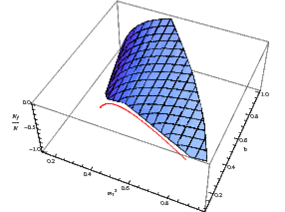
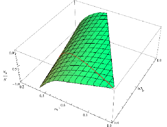
In Fig 7(a) the red line marks the position of the critical points where the three saddles meet, and the first order phase transition ends. The surface marks the locus of points where saddle $III$ becomes dominant. The first order transition takes place when this surface is crossed. Fig 7(b) shows the locus of points where the third order transition takes place⁸⁸ 8 In the figure, the critical line lies on the surface of third order transition points. This is an artifact of our $\mathrm{tr}\,U^{4}$ model and not a generic feature. See Appendix A for more details.. At the parameter values corresponding to a point on this surface the saddle $II$ crosses $\rho_{1}=\frac{1}{2}$. The nature of the saddle solutions is illustrated in Fig 8, for $b=\frac{1}{2}$. The vertical plane is at $\rho_{1}=\frac{1}{2}$. The horizontal plane is a surface of constant temperature. We see that for large enough nonzero $N_{f}/N$, the saddle profile becomes monotonic. So at any temperature there is only one saddle and there is no first order transition. For small $N_{f}/N$ the saddle profile is non-monotonic, so above some temperature $T_{N}$ there are three saddles, and a first order transition takes place. Note that there is always a third order transition at any $N_{f}/N$, and this happens when the constant temperature surface intersects the saddle point solution surface at $\rho_{1}=\frac{1}{2}$.

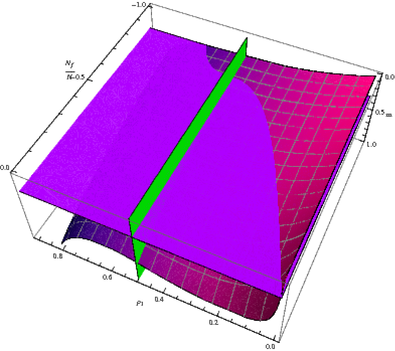
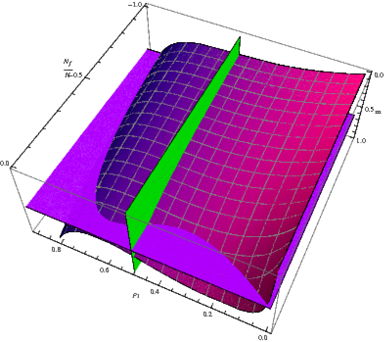
For ease of understanding we present a schematic diagram (Fig 9) of the saddle point dynamics for a fixed coupling ($\lambda$) and varying $N_{f}$ and $T$. The bottom most graph (dotted, graph 1) is where nucleation of saddles $II$ and $III$ take place. The graph (solid, graph 2) above it is the line of first order transitions and the semi-dotted line (graph 3) with arrow is the line of third order transitions. The upper most graph (graph 4) is where the saddle $I$ becomes locally unstable. Three of the graphs (graph 1,2,4) meet and end at a critical point. The critical point itself lies on the line of third order transitions(i.e. graph 3). As noted above this is not a generic feature. It should be noted that the line of third order transitions becomes physical (in the sense that the dominant saddle point passes through it) after the critical point.

References

- [1] Matthew Wingate and Shigemi Ohta. Deconfinement transition and string tensions in SU(4) Yang-Mills theory. Phys. Rev., D63:094502, 2001, hep-lat/0006016.
- [2] F. Karsch, E. Laermann, and A. Peikert. Quark mass and flavor dependence of the QCD phase transition. Nucl. Phys., B605:579–599, 2001, hep-lat/0012023.
- [3] Mikhail A. Stephanov. QCD phase diagram and the critical point. Prog. Theor. Phys. Suppl., 153:139–156, 2004, hep-ph/0402115.
- [4] Juan Martin Maldacena. The large N limit of superconformal field theories and supergravity. Adv. Theor. Math. Phys., 2:231–252, 1998, hep-th/9711200.
- [5] Edward Witten. Anti-de Sitter space, thermal phase transition, and confinement in gauge theories. Adv. Theor. Math. Phys., 2:505–532, 1998, hep-th/9803131.
- [6] S. W. Hawking and Don N. Page. Thermodynamics of Black Holes in anti-De Sitter Space. Commun. Math. Phys., 87:577, 1983.
- [7] Luis Alvarez-Gaume, Cesar Gomez, Hong Liu, and Spenta Wadia. Finite temperature effective action, AdS(5) black holes, and 1/N expansion. Phys. Rev., D71:124023, 2005, hep-th/0502227.
- [8] Ofer Aharony, Joseph Marsano, and Mark Van Raamsdonk. Two loop partition function for large N pure Yang-Mills theory on a small S**3. Phys. Rev., D74:105012, 2006, hep-th/0608156.
- [9] Ofer Aharony, Joseph Marsano, Shiraz Minwalla, Kyriakos Papadodimas, and Mark Van Raamsdonk. A first order deconfinement transition in large N Yang- Mills theory on a small S**3. Phys. Rev., D71:125018, 2005, hep-th/0502149.
- [10] Ofer Aharony et al. The phase structure of low dimensional large N gauge theories on tori. JHEP, 01:140, 2006, hep-th/0508077.
- [11] Andreas Karch and Emanuel Katz. Adding flavor to AdS/CFT. JHEP, 06:043, 2002, hep-th/0205236.
- [12] Sergey A. Cherkis and Akikazu Hashimoto. Supergravity solution of intersecting branes and AdS/CFT with flavor. JHEP, 11:036, 2002, hep-th/0210105.
- [13] Ingo Kirsch and Diana Vaman. The D3/D7 background and flavor dependence of Regge trajectories. Phys. Rev., D72:026007, 2005, hep-th/0505164.
- [14] Benjamin A. Burrington, James T. Liu, Leopoldo A. Pando Zayas, and Diana Vaman. Holographic duals of flavored N = 1 super Yang-Mills: Beyond the probe approximation. JHEP, 02:022, 2005, hep-th/0406207.
- [15] Marta Gomez-Reino, Stephen Naculich, and Howard Schnitzer. Thermodynamics of the localized D2-D6 system. Nucl. Phys., B713:263–277, 2005, hep-th/0412015.
- [16] Howard J. Schnitzer. Confinement / deconfinement transition of large N gauge theories in perturbation theory with N(f) fundamentals: N(f)/N finite. 2006, hep-th/0612099.
- [17] Howard J. Schnitzer. Confinement / deconfinement transition of large N gauge theories with N(f) fundamentals: N(f)/N finite. Nucl. Phys., B695:267–282, 2004, hep-th/0402219.
- [18] Spenta Wadia. A STUDY OF U(N) LATTICE GAUGE THEORY IN TWO-DIMENSIONS. EFI-79/44-CHICAGO.
- [19] D. J. Gross and Edward Witten. Possible Third Order Phase Transition in the Large N Lattice Gauge Theory. Phys. Rev., D21:446–453, 1980.
- [20] Spenta R. Wadia. N = infinity PHASE TRANSITION IN A CLASS OF EXACTLY SOLUBLE MODEL LATTICE GAUGE THEORIES. Phys. Lett., B93:403, 1980.
- [21] Ofer Aharony, Joseph Marsano, Shiraz Minwalla, Kyriakos Papadodimas, and Mark Van Raamsdonk. The Hagedorn / deconfinement phase transition in weakly coupled large N gauge theories. Adv. Theor. Math. Phys., 8:603–696, 2004, hep-th/0310285.
- [22] Bo Sundborg. The Hagedorn transition, deconfinement and N = 4 SYM theory. Nucl. Phys., B573:349–363, 2000, hep-th/9908001.
- [23] Luis Alvarez-Gaume, Pallab Basu, Marcos Marino, and Spenta R. Wadia. Blackhole / string transition for the small Schwarzschild blackhole of AdS(5) x S**5 and critical unitary matrix models. Eur. Phys. J., C48:647–665, 2006, hep-th/0605041.
- [24] G. Veneziano. Some Aspects of a Unified Approach to Gauge, Dual and Gribov Theories. Nucl. Phys., B117:519–545, 1976.
- [25] Gyan Bhanot, Gautam Mandal, and Onuttom Narayan. Phase transitions in one matrix models. Phys. Lett., B251:388–392, 1990.
- [26] Robert D. Pisarski. FINITE TEMPERATURE QCD AT LARGE N. Phys. Rev., D29:1222, 1984.
- [27] Pallab Basu and Spenta R. Wadia. R-charged AdS(5) black holes and large N unitary matrix models. Phys. Rev., D73:045022, 2006, hep-th/0506203.
- [28] Andrew Chamblin, Roberto Emparan, Clifford V. Johnson, and Robert C. Myers. Holography, thermodynamics and fluctuations of charged AdS black holes. Phys. Rev., D60:104026, 1999, hep-th/9904197.
- [29] Matthew Headrick. Hedgehog black holes and the Polyakov loop at strong coupling. 2007, arXiv:0712.4155 [hep-th].
- [30] Felipe Canoura, Paolo Merlatti, and Alfonso V. Ramallo. The supergravity dual of 3d supersymmetric gauge theories with unquenched flavors. 2008, arXiv:0803.1475 [hep-th].
- [31] Roberto Casero, Carlos Nunez, and Angel Paredes. Towards the string dual of N = 1 SQCD-like theories. Phys. Rev., D73:086005, 2006, hep-th/0602027.
- [32] P. Petreczky. QCD thermodynamics on lattice. Nucl. Phys. Proc. Suppl., 140:78–91, 2005, hep-lat/0409139.
- [33] Takehiro Azuma, Pallab Basu, and Anindya Mukherjee. Work in progress.
- [34] E. I. Guendelman and A. Rabinowitz. The Gravitational field of a hedgehog and the evolution of vacuum bubbles. Phys. Rev., D44:3152–3158, 1991.