Effective theory of quadratic degeneracies

In a two-dimensional crystal with a square-lattice ($C_{4v}$) symmetry, it may happen that a pair of bands are degenerate at a point of high symmetry, such as the center ($\Gamma$) or corner (M) of the Brillouin zone. An example of this occurs in a photonic crystal formed by a square lattice of dielectric rods. As shown in Fig. 1(a), the second and third TM bands exhibit a quadratic degeneracy at the M-point. The existence of this degeneracy is independent of details such as the permittivity and radius of the rods, as long as the $C_{4v}$ symmetry is preserved. This degeneracy is of particular interest since Wang et. al. [1] have recently shown that it can be lifted by gyromagnetic effects, which break parity and time-reversal symmetry, and that the bandgap opened in this way is populated by a one-way edge mode analogous to chiral electronic edge states in the quantum Hall effect [2]. Electromagnetic one-way edge modes were first predicted by Haldane and Raghu [3, 4], who argued that they typically occur in systems possessing “Dirac points”, meaning that the modes near each degeneracy point can be described by an effective Dirac Hamiltonian. Although Dirac points have been extensively analyzed in the condensed-matter literature [5], there has been, to the best of our knowledge, no analogous study of these quadratic degeneracies. Since the system proposed by Wang et. al. currently appears to be the most promising for realizing electromagnetic one-way edge modes, due to its large relative bandgap [1], there is a present need for an effective theory of such degeneracies.

In this paper, we present an effective theory that describes the bands near a degeneracy point, based on the symmetry properties of $k$-space around that point. We show that the quadratic degeneracy in the $C_{4v}$ crystal can be regarded as a pair of linear degeneracies, analytically continuable to Dirac points, that are “pinned” to the same $k$-space point by the crystal symmetry. The quadratic degeneracy is robust against perturbations that preserve this symmetry. It can be lifted by parity and time-reversal symmetry breaking (which we will henceforth simply refer to as parity breaking.) In that case, the two bands acquire Chern numbers [3, 4, 6] of $\pm 1$, in agreement with the numerical result of Wang et. al.[1] Breaking the $90^{\circ}$ rotational symmetry “unpins” the quadratic degeneracy point, which splits apart into two distinct linear degeneracies. The theory applies to any two-dimensional Bloch system, whether electronic or photonic, with $C_{4v}$ symmetry and a quadratic degeneracy point. In particular, we show that it accurately describes the aforementioned photonic crystal of dielectric rods for a wide range of dielectric contrasts and rod radii.

Let us consider a crystal in which two bands are degenerate at a point $\vec{k}=\vec{k}_{M}$, with unbroken $C_{4v}$ symmetry. We choose a pair of independent Bloch functions at $\vec{k}_{M}$, denoted by $u_{M}^{1}(\vec{r})$ and $u_{M}^{2}(\vec{r})$. The Bloch functions at neighboring values of $\vec{k}$ can be written as

The mixing elements $c_{nm}(\vec{k})$ can be related to the mode frequencies, $\omega_{n}(\vec{k})$, through an eigenvalue equation

where the “effective Hamiltonian” $H(\vec{k})$ is a $2\times 2$ matrix whose eigenvalues are, by definition, $\lambda_{n}(\vec{k})\equiv\omega_{n}(\vec{k})-\omega_{0}$. We will not be concerned with the value of the “zero-point” frequency $\omega_{0}$. Now, suppose we alter the system that we used for defining $u_{M}^{1}(\vec{r})$ and $u_{M}^{2}(\vec{r})$, such as by breaking some of its symmetries. If the perturbation is sufficiently weak, the Bloch functions of the altered system can still be described by (1) for $\vec{k}\sim\vec{k}_{M}$, with some new choice of $c_{nm}(\vec{k})$ and hence of $H(\vec{k})$.

In this system, we will be interested in three different symmetry-breaking operations. Firstly, we could “shear” the lattice by rotating the basis vectors as follows:

where $a$ denotes the lattice constant. This breaks the symmetry under $C_{4}$ rotations and reflections about the $x$ and $y$ axes. Secondly, we could distort the rods by stretching them along the $x$ or $y$ axes—or, alternatively, stretching the lattice vectors and rescaling $k_{x}$ and/or $k_{y}$; this breaks the symmetry under rotations and reflections about $y=\pm x$. Thirdly, we could break parity, which can be accomplished in a photonic crystal, e.g., using a magneto-optic effect that adds an imaginary off-diagonal term $\mu_{xy}=i\eta$ to the permeability tensor of the rods[1].

The goal is to find an effective Hamiltonian that describes bands such as those in Fig. 1, including the results of the above symmetry-breaking operations. We claim that the desired Hamiltonian has the following form:

where $\vec{\kappa}\equiv\vec{k}-\vec{k}_{M}$ is the $k$-space displacement from the degeneracy point and $\sigma_{i}$ are the usual Pauli matrices. The phenomenological parameter $\lambda_{0}$ determines the frequency scale, $\beta$ and $\gamma$ control the relative curvatures of bands along different directions, $\alpha_{1}$ controls the relative lengths of the two lattice vectors, $\alpha_{2}$ is proportional to the parity-breaking permeability component $\eta$, and $\alpha_{3}$ is proportional to the shear angle $\theta$ defined in (3). This Hamiltonian is valid in the neighborhood of $\kappa=0$, and we have omitted $O(\kappa^{4})$ terms which have negligible effects on the band properties in the regime of interest. Furthermore, we assume that the symmetry-breaking is weak (e.g. $\theta\ll 1$), and thus retain only symmetry-breaking terms that are zeroth-order in $\kappa$.

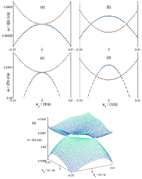
Before discussing the validity of the ansatz (4), let us determine its band structure and then show that it is consistent with the symmetries of the system. First, consider $\alpha_{1}=\alpha_{3}=0$, for which the eigenvalues are

Suppose we assume $\beta=1$ (setting $\beta\neq 1$ simply distorts the bandstructure along the $\kappa_{x}=\pm\kappa_{y}$ directions). For $\alpha_{2}=0$, (5) then reduces to a pair of quadratic bands $\lambda_{\pm}/\lambda_{0}=(\gamma\pm 1)|\vec{\kappa}|^{2}$, which meet at $\vec{\kappa}=0$. The parameter $\gamma$ controls the relative curvatures of the two bands. For instance, when $\gamma=0$, the bands have equal and opposite curvatures, as shown in Fig. 2(a); when $-1<\gamma<0$, the two bands curve in opposite directions but the upper band is flatter, as in Fig. 2(c). Setting $\alpha_{2}\neq 0$ lifts the degeneracy and opens a bandgap $\Delta\lambda=2\lambda_{0}\alpha_{2}$. The two bands will curve in the same direction at $\vec{\kappa}=0$, as observed in Fig. 2 of Wang et. al. [1] and in Fig. 1(b) of the current paper.

Next, let us consider $\alpha_{3}\neq 0$, keeping $\alpha_{1}=0$. For $\alpha_{2}=0$, the quadratic degeneracy splits into two distinct degeneracy points, at $\vec{\kappa}_{\pm}=\pm(\,\sqrt{\alpha_{3}/2},-\sqrt{\alpha_{3}/2}\,)$ for $\alpha_{3}>0$ and $\vec{\kappa}_{\pm}=\pm(\,\sqrt{-\alpha_{3}/2},\sqrt{-\alpha_{3}/2}\,)$ for $\alpha_{3}<0$. We will henceforth assume that $\alpha_{3}>0$; the following discussion can be easily adapted to the $\alpha_{3}<0$ case. Let us expand the Hamiltonian around $\vec{\kappa}_{\pm}$, using the variables

which are simply $k$-space displacements from $\vec{\kappa}_{\pm}$, rotated by $45^{\circ}$. To first order in $q_{1}$ and $q_{2}$,

When $\gamma=0$ and $\beta=1$, this reduces to a two-dimensional Dirac Hamiltonian near each each degeneracy point (or “Dirac point”). Furthermore, $\alpha_{2}$ plays the role of a mass term, opening a bandgap $\Delta\lambda=2\lambda_{0}\alpha_{2}$. Setting $\gamma\neq 0$ distorts the Dirac Hamiltonian and its eigenvalue spectrum; for example, the Dirac cones in the $\alpha_{2}=0$ limit become tilted in $k$-space, as shown in Fig. 2(d). Along the line $\kappa_{y}=\pm\kappa_{x}$, the splitting of the degeneracy point can be thought of as a vertical relative displacement of the two parabolic bands (note, however, that the bands meet only at isolated points in the full $\kappa$-space.) The splitting is accompanied by a change in the density of states from a discontinuity to a linear “dip” centered at the frequency of the band degeneracy. When $\alpha_{2}\neq 0$, the density of (TM) states is discontinuous at the band edges, dropping to zero inside the band gap.

The situation is very similar for $\alpha_{1}\neq 0$. When $\alpha_{2}=\alpha_{3}=0$, the degeneracy splits into two, but along the line $\kappa_{y}=0$ (if $\alpha_{1}>0$) or $\kappa_{x}=0$ (if $\alpha_{1}<0$), instead of $\kappa_{x}=\pm\kappa_{y}$. When both $\alpha_{1}$ and $\alpha_{3}$ are nonzero, the degeneracies are located at an intermediate location, $\kappa_{\pm}=\pm(\alpha_{1}^{2}+\alpha_{3}^{2})^{1/4}(\cos\phi,\sin\phi)$, where $\tan\phi=\alpha_{3}/\alpha_{1}$, and expanding around each point yields a Dirac-like Hamiltonian analogous to (7).

When $\alpha_{2}\neq 0$, the bands are non-degenerate, and their Chern numbers [6] can be calculated. The details of this calculation are given in the Appendix, and the result is that the upper and lower bands possess Chern numbers $-\mathrm{sgn}(\alpha_{2})$ and $\mathrm{sgn}(\alpha_{2})$ respectively, regardless of the values of $\alpha_{1}$, $\alpha_{3}$, $\beta$, and $\gamma$. This implies the existence of a single family of one-way edge modes [7], and agrees exactly with the numerical results of Wang et. al.[1]. Although the effective Hamiltonian (4) is only valid near $\kappa=0$, it yields the same Chern number as the actual bandstructure because only the region near the broken degeneracy point provides a non-vanishing “Berry flux” contribution to the Chern number [6, 3, 4]. Furthermore, while our theory only describes weak symmetry-breaking, the Chern number is a topological quantity and cannot be altered by non-perturbative distortions (as long as the bands remain non-degenerate [6]), which is why it remains unchanged even in the strong parity-breaking regime explored by Wang et. al. When $\alpha_{1}$ and/or $\alpha_{3}$ are non-zero, the two linear degeneracy points each contribute $\pm 1/2$ to the Chern number, in accordance with previous analyses of the Dirac Hamiltonian [5]. When $\alpha_{1}=\alpha_{3}=0$, the Berry connection winds twice as fast around the point $\kappa=0$, which provides the entire contribution of $\pm 1$. The dependence of the Chern number on the sign of $\alpha_{2}$ confirms that $\alpha_{2}$ controls parity breaking, since the Chern number can be shown to vanish identically when parity is unbroken.

The fully symmetric Hamiltonian $H_{0}\equiv H|_{\alpha_{i}=0}$ must transform under any operation $g\in C_{4v}$ as

Regardless of the values of $\beta$, $\gamma$, and $\lambda_{0}$, this holds if $D(g)$ falls under $E$, the only two-dimensional irreducible representation of $C_{4v}$. Thus, $\pm 90^{\circ}$ rotations can be represented by $\mp i\sigma_{2}$, reflections about the $\kappa_{x}$ ($\kappa_{y}$) axes by $\sigma_{1}$ ($-\sigma_{1}$), and reflections about $\kappa_{y}=\pm\kappa_{x}$ by $\pm\sigma_{3}$.

By studying how $H(\vec{\kappa})$ transforms under $E$, we can show that the quadratic degeneracy is protected by the crystal symmetry. Any zeroth-order term proportional to the identity matrix, when added to $H_{0}$, simply shifts the eigenvalues without opening a gap. Adding a zeroth-order term proportional to $\sigma_{1}$ (i.e. $\alpha_{1}\neq 0$) breaks $C_{4v}$ since, under the representation $E$, $\alpha\rightarrow-\alpha$ for $90^{\circ}$ rotations and reflections across $\kappa_{x}=\pm\kappa_{y}$. Note that $\alpha\rightarrow\alpha$ for reflections across the $\kappa_{x}$ and $\kappa_{y}$ axes, in agreement with our claim that $\alpha_{1}\neq 0$ corresponds to stretching the lattice. Similarly, setting $\alpha_{2}\neq 0$ preserves the rotational symmetries but breaks the reflection symmetries (parity). Finally, setting $\alpha_{3}\neq 0$ preserves the reflection symmetry across $\kappa_{x}=\pm\kappa_{y}$ but breaks the symmetry under $90^{\circ}$ rotations and reflections across $\kappa_{x}=0$ and $\kappa_{y}=0$.

Furthermore, the Hamiltonian cannot include terms that are first-order in $\vec{\kappa}$ if the $C_{4v}$ symmetry is unbroken or only partially broken. Such terms have the general form $\Delta H=\sum_{i=1}^{2}\sum_{j=1}^{3}\kappa_{i}c_{ij}\sigma_{j}$, and we can show that $c_{ij}=0$ for all $i,j$ as long as the system is symmetric under either rotations, reflections about the $\kappa_{x}$ and $\kappa_{y}$ axes, or reflections about $\kappa_{x}=\pm\kappa_{y}$. At least one of these symmetries is preserved by each of the three “elementary” distortions discussed above. This situation may be contrasted with a triangular or honeycomb lattice, for which there is a $C_{3v}$ symmetry around each corner of the hexagonal Brillouin zone. There, one can write down an $O(\kappa)$ Hamiltonian which transforms under a two-dimensional irreducible representation of $C_{3v}$: this is just the Dirac Hamiltonian

In this case, a zeroth-order “mass” term proportional to $\sigma_{2}$ controls parity breaking [5].

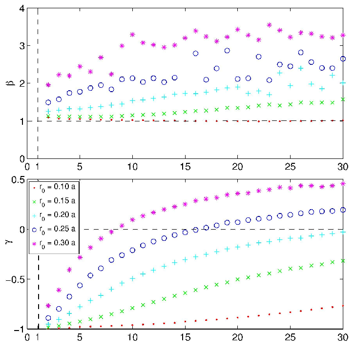
We checked the validity of the ansatz (4) and computed the parameters $\alpha_{i}$, $\beta$, and $\gamma$ using the MPB [8] and COMSOL [9] computer programs, which solve the Maxwell equations without any approximations apart from the discretization of the simulation cell. We first determined $\beta$ and $\gamma$ for $\alpha_{1}=\alpha_{2}=\alpha_{3}=0$ by fitting the computed bandstructures of the fully-symmetric crystal to (5). As shown in Fig. 3, we obtain values for $\beta$ and $\gamma$ that depend on the details of the crytal, including the rod radius and permittivity.

Upon perturbing the simulated crystals by changing the lattice constant slightly along (say) the $x$ direction, $\delta a_{x}<0$, the degeneracy splits along the line $\kappa_{y}=0$ in the computed bandstructures. From the location of the linear degeneracies, we can obtain $\alpha_{1}$, which turns out to be proportional to $\delta a_{x}$. Similarly, setting $\theta\neq 0$ induces linear degeneracies along the line $\kappa_{x}=\kappa_{y}$, and $\alpha_{3}$ is found to be proportional to $\theta$. By computing the bands for off-diagonal permeability component $\mu_{xy}=i\eta$ in the rods, and fitting these to (5), we find that $\alpha_{2}$ is proportional to $\eta$. These results are shown in Fig. 4. Like $\beta$ and $\gamma$, the proportionality factors $\alpha_{1}/\delta a_{x}$, $\alpha_{2}/\eta$, and $\alpha_{3}/\theta$ depend on the details of the crystal. The fact that the linear degeneracies induced by $\alpha_{3}\neq 0$ are not determined solely by the lattice geometry stands in contrast to Dirac points in previously-studied triangular and hexagonal lattices, which are pinned to the corners of the Brillouin zone.

In conclusion, we have presented an effective theory for a pair of bands in the vicinity of a band degeneracy, within a two-dimensional $C_{4v}$-symmetric crystal. The high degree of symmetry near the degeneracy point determines the form of the $2\times 2$ effective Hamiltonian matrix, including the lowest-order symmetry-breaking terms. In particular, we showed that quadratic nature of the degeneracy is protected by the $C_{4v}$ symmetry. We have also shown that the theory accurately describes the second and third TM bands of square-lattice photonic crystals near their M-point degeneracy, including the correct Chern numbers when parity is broken [1]. On the other hand, the theory should be applicable to any electronic or photonic system possessing $C_{4v}$ symmetry and a two-fold band degeneracy; it is possible, for instance, to construct tight-binding electronic models that reduce to our effective Hamiltonian (4) near a degeneracy point. The advantage of the present method is that it relies only on symmetry principles, and can therefore be applied to systems, such as photonic crystals, where other methods such as tight-binding are not applicable. For lattice symmetries other than $C_{4v}$, effective Hamiltonians can be constructed by finding an appropriate representation of the symmetry group.

*

References

- [1] Z. Wang, Y. D. Chong, J. D. Joannopoulos, and M. Soljačić, Phys. Rev. Lett. 100, 013905 (2008).
- [2] R. E. Prange and S. M. Girvin, ed. The Quantum Hall Effect. (Springer-Verlag, New York, 1987).
- [3] F. D. M. Haldane and S. Raghu, Phys. Rev. Lett. 100, 013904 (2008).
- [4] S. Raghu and F. D. M. Haldane, cond-mat/0602501.
- [5] F. D. M. Haldane, Phys. Rev. Lett. 61, 2015 (1988).
- [6] B. Simon, Phys. Rev. Lett. 51, 2167 (1983).
- [7] Y. Hatsugai, Phys. Rev. Lett. 71, 3697 (1993).
- [8] S. G. Johnson and J. D. Joannopoulos, Opt. Express 8 173 (2001).
- [9] Comsol Multiphysics 3.3, COMSOL Inc. www.comsol.com.