Self-Assembly of Discrete Self-Similar Fractals (Extended Abstract)

This research was supported in part by National Science Foundation Grants 0652569 and 0728806

Matthew J. Patitz Scott M. Summers Affiliation: Iowa State University, Ames, IA 50011, USA Email: {mpatitz,summers}@cs.iastate.edu

Abstract

In this paper, we search for absolute limitations of the Tile Assembly Model (TAM), along with techniques to work around such limitations. Specifically, we investigate the self-assembly of fractal shapes in the TAM. We prove that no self-similar fractal fully weakly self-assembles at temperature 1, and that certain kinds of self-similar fractals do not strictly self-assemble at any temperature. Additionally, we extend the fiber construction from Lathrop et. al. (2007) to show that any self-similar fractal belonging to a particular class of “nice” self-similar fractals has a fibered version that strictly self-assembles in the TAM.

1 Introduction

Self-assembly is a bottom-up process by which (usually a small number of) fundamental components automatically coalesce to form a target structure. In 1998, Winfree [18] introduced the (abstract) Tile Assembly Model (TAM) - an extension of Wang tiling [16, 17], and a mathematical model of the DNA self-assembly pioneered by Seeman et. al. [14]. In the TAM, the fundamental components are un-rotatable, but translatable “tile types” whose sides are labeled with glue “colors” and “strengths.” Two tiles that are placed next to each other interact if the glue colors on their abutting sides match, and they bind if the strength on their abutting sides matches, and is at least a certain “temperature.” Rothemund and Winfree [13, 12] later refined the model, and Lathrop et. al. [10] gave a treatment of the TAM in which equal status is bestowed upon the self-assembly of infinite and finite structures. There are also several generalizations [2, 11, 8] of the TAM.

Despite its deliberate over-simplification, the TAM is a computationally and geometrically expressive model. For instance, Winfree [18] proved that the TAM is computationally universal, and thus can be directed algorithmically. Winfree [18] also exhibited a seven-tile-type self-assembly system, directed by a clever XOR-like algorithm, that “paints” a picture of a well-known shape, the discrete Sierpinski triangle $\mathbf{S}$ , onto the first quadrant. Note that the underlying shapes of each of the previous results are actually infinite canvases that completely cover the first quadrant, onto which computationally interesting shapes are painted (i.e., full weak self-assembly). Moreover, Lathrop et. al [9] recently gave a new characterization of the computably enumerable sets in terms of weak self-assembly using a “ray construction.” It is natural to ask the question: How expressive is the TAM with respect to the self-assembly of a particular, possibly infinite shape, and nothing else (i.e., strict self-assembly)?

In the case of strict self-assembly of finite shapes, the TAM certainly remains an interesting model, so long as the size (tile complexity) of the assembly system is required to be “small” relative to the shape that it ultimately produces. For instance, Rothemund and Winfree [13] proved that there are small tile sets in which large squares self-assemble. Moreover, Soloveichik and Winfree [15] established the remarkable fact that, if one is not concerned with the scale of an “algorithmically describable” finite shape, then there is always a small tile set in which the shape self-assembles. Note that if the tile complexity of an assembly system is unbounded, then every finite shape trivially (but perhaps not feasibly) self-assembles.

When the tile complexity of an assembly system is unbounded (yet finite), only infinite shapes are of interest. In the case of strict self-assembly of infinite shapes, the power of the TAM has only recently been investigated. Lathrop et. al. [10] established that self-similar tree shapes do not strictly self-assemble in the TAM given any finite number of tile types. A “fiber construction” is also given in [10], which strictly self-assembles a non-trivial fractal structure.

In this paper, we search for (1) absolute limitations of the TAM, with respect to the strict self-assembly of shapes, and (2) techniques that allow one to “work around” such limitations. Specifically, we investigate the strict self-assembly of fractal shapes in the TAM. We prove three main results: two negative and one positive. Our first negative (i.e., impossibility) result says that no self-similar fractal fully weakly self-assembles in the TAM (at temperature 1). In our second impossibility result, we exhibit a class of discrete self-similar fractals, to which the standard discrete Sierpinski triangle belongs, that do not strictly self-assemble in the TAM (at any temperature). Finally, in our positive result, we use simple modified counters to extend the fiber construction from Lathrop et. al. [10] to a particular class of discrete self-similar fractals.

2 Preliminaries

2.1 Notation and Terminology

We work in the discrete Euclidean plane $\mathbb{Z}^{2}=\mathbb{Z}\times\mathbb{Z}$ . We write $U_{2}$ for the set of all unit vectors, i.e., vectors of length $1$ , in $\mathbb{Z}^{2}$ . We regard the four elements of $U_{2}$ as (names of the cardinal) directions in $\mathbb{Z}^{2}$ .

We write $[X]^{2}$ for the set of all $2$ -element subsets of a set $X$ . All graphs here are undirected graphs, i.e., ordered pairs $G=(V,E)$ , where $V$ is the set of vertices and $E\subseteq[V]^{2}$ is the set of edges. A cut of a graph $G=(V,E)$ is a partition $C=(C_{0},C_{1})$ of $V$ into two nonempty, disjoint subsets $C_{0}$ and $C_{1}$ .

A binding function on a graph $G=(V,E)$ is a function $\beta:E\rightarrow\mathbb{N}$ . (Intuitively, if $\{u,v\}\in E$ , then $\beta\left(\{u,v\}\right)$ is the strength with which $u$ is bound to $v$ by $\{u,v\}$ according to $\beta$ . If $\beta$ is a binding function on a graph $G=(V,E)$ and $C=(C_{0},C_{1})$ is a cut of $G$ , then the binding strength of $\beta$ on $C$ is

\beta_{C}=\left\{\beta(e)\left|e\in E,e\cap C_{0}\neq\emptyset,\textmd{ and }e\cap C_{1}\neq\emptyset\right.\right\}.

The binding strength of $\beta$ on the graph $G$ is then

\beta(G)=\min\left\{\beta_{C}\left|C\textmd{ is a cut of }G\right.\right\}.

A binding graph is an ordered triple $G=(V,E,\beta)$ , where $(V,E)$ is a graph and $\beta$ is a binding function on $(V,E)$ . If $\tau\in\mathbb{N}$ , then a binding graph $G=(V,E,\beta)$ is $\tau$ -stable if $\beta(V,E)\geq\tau$ .

A grid graph is a graph $G=(V,E)$ in which $V\subseteq\mathbb{Z}^{2}$ and every edge $\{\vec{m},\vec{n}\}\in E$ has the property that $\vec{m}-\vec{n}\in U_{2}$ . The full grid graph on a set $V\subseteq\mathbb{Z}^{2}$ is the graph $G^{\#}_{V}=(V,E)$ in which $E$ contains every $\{\vec{m},\vec{n}\}\in[V]^{2}$ such that $\vec{m}-\vec{n}\in U_{2}$ .

We say that $f$ is a partial function from a set $X$ to a set $Y$ , and we write $f:X\dashrightarrow Y$ , if $f:D\rightarrow Y$ for some set $D\subseteq X$ . In this case, $D$ is the domain of $f$ , and we write $D={\rm dom}\;{f}$ .

All logarithms here are base-2.

2.2 The Tile Assembly Model

We review the basic ideas of the Tile Assembly Model. Our development largely follows that of [13, 12], but some of our terminology and notation are specifically tailored to our objectives. In particular, our version of the model only uses nonnegative “glue strengths”, and it bestows equal status on finite and infinite assemblies. We emphasize that the results in this section have been known for years, e.g., they appear, with proofs, in [12].

Definition.

A tile type over an alphabet $\Sigma$ is a function $t:U_{2}\rightarrow\Sigma^{*}\times\mathbb{N}$ . We write $t=({\rm col}_{t},{\rm str}_{t})$ , where ${\rm col}_{t}:U_{2}\rightarrow\Sigma^{*}$ , and ${\rm str}_{t}:U_{2}\rightarrow\mathbb{N}$ are defined by $t(\vec{u})=({\rm col}_{t}(\vec{u}),{\rm str}_{t}(\vec{u}))$ for all $\vec{u}\in U_{2}$ .

Intuitively, a tile of type $t$ is a unit square. It can be translated but not rotated, so it has a well-defined “side $\vec{u}\;$ ” for each $\vec{u}\in U_{2}$ . Each side $\vec{u}$ of the tile is covered with a “glue” of color ${\rm col}_{t}(\vec{u})$ and strength ${\rm str}_{t}(\vec{u})$ . If tiles of types $t$ and $t^{\prime}$ are placed with their centers at $\vec{m}$ and $\vec{m}+\vec{u}$ , respectively, where $\vec{m}\in\mathbb{Z}^{2}$ and $\vec{u}\in U_{2}$ , then they will bind with strength ${\rm str}_{t}(\vec{u})\cdot[\![t(\vec{u})=t^{\prime}(-\vec{u})]\!]$ where $[\![\phi]\!]$ is the Boolean value of the statement $\phi$ . Note that this binding strength is $0$ unless the adjoining sides have glues of both the same color and the same strength.

For the remainder of this section, unless otherwise specified, $T$ is an arbitrary set of tile types, and $\tau\in\mathbb{N}$ is the “temperature.”

Definition.

A T-configuration is a partial function $\alpha:\mathbb{Z}^{2}\dashrightarrow T$ .

Intuitively, a configuration is an assignment $\alpha$ in which a tile of type $\alpha(\vec{m})$ has been placed (with its center) at each point $\vec{m}\in{\rm dom}\;\alpha$ . The following data structure characterizes how these tiles are bound to one another.

Definition.

The binding graph of a $T$ -configuration $\alpha:\mathbb{Z}^{2}\dashrightarrow T$ is the binding graph $G_{\alpha}=(V,E,\beta)$ , where $(V,E)$ is the grid graph given by

	$\displaystyle V=\;$	$\displaystyle{\rm dom}\;\alpha\text{,}$
	$\displaystyle E=\;$	$\displaystyle\left\{\left.\{\vec{m},\vec{n}\}\in{[V]}^{2}\right\|\vec{m}-\vec{n}\in U_{n},{\rm col}_{\alpha(\vec{m})}\left(\vec{n}-\vec{m}\right)={\rm col}_{\alpha(\vec{n})}\left(\vec{m}-\vec{n}\right),\text{and }{\rm str}_{\alpha(\vec{m})}\left(\vec{n}-\vec{m}\right)>0\right\},$

and the binding function $\beta:E\rightarrow\mathbb{Z}^{+}$ is given by

\beta\left(\{\vec{m},\vec{n}\}\right)={\rm str}_{\alpha(\vec{m})}\left(\vec{n}-\vec{m}\right)

for all $\left\{\vec{m},\vec{n}\right\}\in E$ .

Definition.

1.

A $T$ -configuration $\alpha$ is $\tau$ -stable if its binding graph $G_{\alpha}$ is $\tau$ -stable.
2.

A $\tau$ - $T$ -assembly is a $T$ -configuration that is $\tau$ -stable. We write $\mathcal{A}^{\tau}_{T}$ for the set of all $\tau$ - $T$ -assemblies.

Definition.

Let $\alpha$ and $\alpha^{\prime}$ be $T$ -configurations.

1.

$\alpha$ is a subconfiguration of $\alpha^{\prime}$ , and we write $\alpha\sqsubseteq\alpha^{\prime}$ , if ${\rm dom}\;\alpha\subseteq{\rm dom}\;\alpha^{\prime}$ and, for all $\vec{m}\in{\rm dom}\;\alpha$ , $\alpha(\vec{m})=\alpha^{\prime}(\vec{m}).$
2.

$\alpha^{\prime}$ is a single-tile extension of $\alpha$ if $\alpha\sqsubseteq\alpha^{\prime}$ and ${\rm dom}\;\alpha^{\prime}-{\rm dom}\;\alpha$ is a singleton set. In this case, we write $\alpha^{\prime}=\alpha+(\vec{m}\mapsto t)$ , where $\{\vec{m}\}={\rm dom}\;\alpha^{\prime}-{\rm dom}\;\alpha$ and $t=\alpha^{\prime}(\vec{m})$ .

Note that the expression $\alpha+(\vec{m}\mapsto t)$ is only defined when $\vec{m}\in\mathbb{Z}^{2}-{\rm dom}\;\alpha$ .

We next define the “ $\tau$ - $t$ -frontier” of a $\tau$ - $T$ -assembly $\alpha$ to be the set of all positions at which a tile of type $t$ can be “ $\tau$ -stably added” to the assembly $\alpha$ .

Definition.

Let $\alpha\in\mathcal{A}^{\tau}_{T}$ .

For each $t\in T$ , the $\tau$ - $t$ -frontier of $\alpha$ is the set

{\partial}^{\tau}_{t}{\alpha}=\left\{\vec{m}\in\mathbb{Z}^{2}-{\rm dom}\;\alpha\left|\;\sum_{\vec{u}\in U_{2}}{\rm str}_{t}(\vec{u})\cdot\left[\!\left[\alpha(\vec{m}+\vec{u})(-\vec{u})=t(\vec{u})\right]\!\right]\geq\tau\right.\right\}.

2.

The $\tau$ -frontier of $\alpha$ is the set

${\partial}^{\tau}{\alpha}=\bigcup_{t\in T}{\partial}^{\tau}_{t}{\alpha}.$

The following lemma shows that the definition of ${\partial}^{\tau}_{t}{\alpha}$ achieves the desired effect.

Lemma 1.

Let $\alpha\in\mathcal{A}^{\tau}_{T}$ , $\vec{m}\in\mathbb{Z}^{2}-{\rm dom}\;\alpha$ , and $t\in T$ . Then $\alpha+(\vec{m}\mapsto t)\in\mathcal{A}^{\tau}_{T}$ if and only if $\vec{m}\in{\partial}^{\tau}_{t}{\alpha}$ .

Notation.

We write $\alpha\xrightarrow[\tau,T]{1}\alpha^{\prime}$ (or, when $\tau$ and $T$ are clear from context, $\alpha\stackrel{{\scriptstyle 1}}{{\longrightarrow}}\alpha^{\prime}$ ) to indicate that $\alpha,\alpha^{\prime}\in\mathcal{A}^{\tau}_{T}$ and $\alpha^{\prime}$ is a single-tile extension of $\alpha$ .

In general, self-assembly occurs with tiles adsorbing nondeterministically and asynchronously to a growing assembly. We now define assembly sequences, which are particular “execution traces” of how this might occur.

Definition.

A $\tau$ - $T$ -assembly sequence is a sequence $\vec{\alpha}=(\alpha_{i}\mid 0\leq i<k)$ in $\mathcal{A}^{\tau}_{T}$ , where $k\in\mathbb{Z}^{+}\cup\{\infty\}$ and, for each $i$ with $1\leq i+1<k$ , $\alpha_{i}\xrightarrow[\tau,T]{1}\alpha_{i+1}$ .

Note that assembly sequences may be finite or infinite in length. Note also that, in any $\tau$ - $T$ -assembly sequence $\vec{\alpha}=(\alpha_{i}\mid 0\leq i<k)$ , we have $\alpha_{i}\sqsubseteq\alpha_{j}$ for all $0\leq i\leq j<k$ .

Definition.

The result of a $\tau$ - $T$ -assembly sequence $\vec{\alpha}=(\alpha_{i}\mid 0\leq i<k)$ is the unique $T$ -configuration $\alpha=\textrm{res}(\vec{\alpha})$ satisfying ${\rm dom}\;\alpha=\bigcup_{0\leq i<k}{{\rm dom}\;\alpha_{i}}$ and $\alpha_{i}\sqsubseteq\alpha$ for each $0\leq i<k$ .

It is clear that $\textrm{res}(\vec{\alpha})\in\mathcal{A}^{\tau}_{T}$ for every $\tau$ - $T$ -assembly sequence $\vec{\alpha}$ .

Definition.

Let $\alpha,\alpha^{\prime}\in\mathcal{A}^{\tau}_{T}$ .

1.

A $\tau$ - $T$ -assembly sequence from $\alpha$ to $\alpha^{\prime}$ is a $\tau$ - $T$ -assembly sequence $\vec{\alpha}=(\alpha_{i}\mid 0\leq i<k)$ such that $\alpha_{0}=\alpha$ and $\textrm{res}(\vec{\alpha})=\alpha^{\prime}$ .
2.

We write $\alpha\xrightarrow[\tau,T]{}\alpha^{\prime}$ (or, when $\tau$ and $T$ are clear from context, $\alpha\longrightarrow\alpha^{\prime}$ ) to indicate that there exists a $\tau$ - $T$ -assembly sequence from $\alpha$ to $\alpha^{\prime}$ .

Definition.

An assembly $\alpha\in\mathcal{A}^{\tau}_{T}$ is terminal if and only if $\partial^{\tau}{\alpha}=\emptyset$ .

We now define tile assembly systems.

Definition.

1.

A generalized tile assembly system (GTAS) is an ordered triple

$\mathcal{T}=(T,\sigma,\tau),$

where $T$ is a set of tile types, $\sigma\in\mathcal{A}^{\tau}_{T}$ is the seed assembly, and $\tau\in\mathbb{N}$ is the temperature.
2.

A tile assembly system (TAS) is a GTAS $\mathcal{T}=(T,\sigma,\tau)$ in which the sets $T$ and ${\rm dom}\;\sigma$ are finite.

Intuitively, a “run” of a GTAS $\mathcal{T}=(T,\sigma,\tau)$ is any $\tau$ - $T$ -assembly sequence $\vec{\alpha}=(\alpha_{i}\mid 0\leq i<k)$ that begins with $\alpha_{0}=\sigma$ . Accordingly, we define the following sets.

Definition.

Let $\mathcal{T}=(T,\sigma,\tau)$ be a GTAS.

1.

The set of assemblies produced by $\mathcal{T}$ is

$\mathcal{A}[\mathcal{T}]=\left\{\alpha\in\mathcal{A}^{\tau}_{T}\left|\sigma\xrightarrow[\tau,T]{}\alpha\right.\right\}.$
2.

The set of terminal assemblies produced by $\mathcal{T}$ is

$\mathcal{A}_{\Box}[\mathcal{T}]=\left\{\left.\alpha\in\mathcal{A}[\mathcal{T}]\right|\alpha\textrm{ is terminal}\right\}.$

Definition.

A GTAS $\mathcal{T}=(T,\sigma,\tau)$ is directed if $\left|\mathcal{A}_{\Box}[\mathcal{T}]\right|=1$ .

We are using the terminology of the mathematical theory of relations here. The reader is cautioned that the term ”directed” has also been used for a different, more specialized notion in self-assembly [AKKR02].

In the present paper, we are primarily interested in the self-assembly of sets.

Definition.

Let $\mathcal{T}=(T,\sigma,\tau)$ be a GTAS, and let $X\subseteq\mathbb{Z}^{2}$ .

1.

The set $X$ weakly self-assembles in $\mathcal{T}$ if there is a set $B\subseteq T$ such that, for all $\alpha\in\mathcal{A}_{\Box}[\mathcal{T}]$ , $\alpha^{-1}(B)=X$ .
2.

The set $X$ fully weakly self-assembles in $\mathcal{T}$ if $X$ and $\mathbb{Z}^{2}-X$ both weakly self-assemble.
3.

The set $X$ strictly self-assembles in $\mathcal{T}$ if, for all $\alpha\in\mathcal{A}_{\Box}[\mathcal{T}]$ , ${\rm dom}\;\alpha=X$ .

Intuitively, a set $X$ weakly self-assembles in $\mathcal{T}$ if there is a designated set $B$ of “black” tile types such that every terminal assembly of $\mathcal{T}$ “paints the set $X$ - and only the set $X$ - black”. Moreover, a set fully weakly self-assembles in $\mathcal{T}$ if every terminal assembly of $\mathcal{T}$ tiles the entire plane on top of which $X$ is “painted.” In contrast, a set $X$ strictly self-assembles in $\mathcal{T}$ if every terminal assembly of $\mathcal{T}$ has tiles on the set $X$ and only on the set $X$ . Clearly, every set that strictly self-assembles in a GTAS $\mathcal{T}$ also weakly self-assembles in $\mathcal{T}$ .

We now have the machinery to say what it means for a set in the discrete Euclidean plane to self-assemble in either the fully weak, weak or the strict sense.

Definition.

Let $X\subseteq\mathbb{Z}^{2}$ .

1.

The set $X$ weakly self-assembles if there is a TAS $\mathcal{T}$ such that $X$ weakly self-assembles in $\mathcal{T}$ .
2.

The set $X$ fully weakly self-assembles if there is a TAS $\mathcal{T}$ such that $X$ fully weakly self-assembles in $\mathcal{T}$ .
3.

The set $X$ strictly self-assembles if there is a TAS $\mathcal{T}$ such that $X$ strictly self-assembles in $\mathcal{T}$ .

Note that $\mathcal{T}$ is required to be a TAS, i.e., finite, in all three parts of the above definition.

2.3 Local Determinism

The proof of our construction uses the local determinism method of Soloveichik and Winfree [15], which we now review.

Notation.

For each $T$ -configuration $\alpha$ , each $\vec{m}\in\mathbb{Z}^{2}$ , and each $\vec{u}\in U_{2}$ ,

\text{str}_{\alpha}(\vec{m},\vec{u})=\text{str}_{\alpha(\vec{m})}(\vec{u})\cdot[\![\alpha(\vec{m})(\vec{u})=\alpha(\vec{m}+\vec{u})(-\vec{u})]\!].

(The Boolean value on the right is 0 if $\{\vec{m},\vec{m}+\vec{u}\}\nsubseteq{\rm dom}\;{\alpha}$ .)

Notation.

If $\vec{\alpha}=(\alpha_{i}\;|\;0\leq i<k)$ is a $\tau$ - $T$ -assembly sequence and $\vec{m}\in\mathbb{Z}^{2}$ , then the $\vec{\alpha}$ -index of $\vec{m}$ is

i_{\vec{\alpha}}(\vec{m})=\min\{i\in\mathbb{N}\;\left|\;\vec{m}\in{\rm dom}\;{\alpha_{i}}\right.\}.

Observation 1.

$\vec{m}\in{\rm dom}\;{\textrm{res}(\vec{\alpha})}\Leftrightarrow i_{\vec{\alpha}}(\vec{m})<\infty$ .

Notation.

If $\vec{\alpha}=(\alpha_{i}\;|\;0\leq i<k)$ is a $\tau$ - $T$ -assembly sequence, then, for $\vec{m},\vec{m}^{\prime}\in\mathbb{Z}^{2}$ ,

\vec{m}\prec_{\vec{\alpha}}\vec{m}^{\prime}\Leftrightarrow i_{\vec{\alpha}}(\vec{m})<i_{\vec{\alpha}}(\vec{m}^{\prime}).

Definition.

(Soloveichik and Winfree [15]) Let $\vec{\alpha}=(\alpha_{i}\;|\;0\leq i<k)$ be a $\tau$ - $T$ -assembly sequence, and let $\alpha=\textrm{res}(\vec{\alpha})$ . For each location $\vec{m}\in{\rm dom}\;{\alpha}$ , define the following sets of directions.

1.

$\textmd{IN}^{\vec{\alpha}}(\vec{m})=\left\{\vec{u}\in U_{2}\left|\vec{m}+\vec{u}\prec_{\vec{\alpha}}\vec{m}\textmd{ and }\textmd{str}_{\alpha_{i_{\vec{\alpha}}(\vec{m})}}(\vec{m},\vec{u})>0\right.\right\}$ .
2.

$\textmd{OUT}^{\vec{\alpha}}(\vec{m})=\left\{\vec{u}\in U_{2}\left|-\vec{u}\in\textmd{IN}^{\vec{\alpha}}(\vec{m}+\vec{u}\right.)\right\}$ .

Intuitively, $\textmd{IN}^{\vec{\alpha}}(\vec{m})$ is the set of sides on which the tile at $\vec{m}$ initially binds in the assembly sequence $\vec{\alpha}$ , and $\textmd{OUT}^{\vec{\alpha}}(\vec{m})$ is the set of sides on which this tile propagates information to future tiles.

Note that $\textmd{IN}^{\vec{\alpha}}(\vec{m})=\emptyset$ for all $\vec{m}\in\alpha_{0}$ .

Notation.

If $\vec{\alpha}=(\alpha_{i}\;|\;0\leq i<k)$ is a $\tau$ - $T$ -assembly sequence, $\alpha=\textrm{res}(\vec{\alpha})$ , and $\vec{m}\in{\rm dom}\;{\alpha}-{\rm dom}\;{\alpha_{0}}$ , then

\vec{\alpha}\setminus\vec{m}=\alpha\upharpoonright\left({\rm dom}\;{\alpha}-\{\vec{m}\}-\left(\vec{m}+\textmd{OUT}^{\vec{\alpha}}(\vec{m})\right)\right).

(Note that $\vec{\alpha}\setminus\vec{m}$ is a $T$ -configuration that may or may not be a $\tau$ - $T$ -assembly.

Definition.

(Soloveichik and Winfree [15]). A $\tau$ - $T$ -assembly sequence $\vec{\alpha}=(\alpha_{i}\;|\;0\leq i<k)$ with result $\alpha$ is locally deterministic if it has the following three properties.

1.

For all $\vec{m}\in{\rm dom}\;{\alpha}-{\rm dom}\;{\alpha_{0}}$ ,

$\sum_{\vec{u}\in\textmd{IN}^{\vec{\alpha}}(\vec{m})}{\textmd{str}_{\alpha_{i_{\vec{\alpha}}(\vec{m})}}(\vec{m},\vec{u})}=\tau.$
2.

For all $\vec{m}\in{\rm dom}\;{\alpha}-{\rm dom}\;{\alpha_{0}}$ and all $t\in T-\{\alpha(\vec{m})\}$ , $\vec{m}\not\in{\partial}^{\tau}_{t}{\left(\vec{\alpha}\setminus\vec{m}\right)}$ .
3.

$\partial^{\tau}{\alpha}=\emptyset$ .

That is, $\vec{\alpha}$ is locally deterministic if (1) each tile added in $\vec{\alpha}$ “just barely” binds to the assembly; (2) if a tile of type $t_{0}$ at a location $\vec{m}$ and its immediate “OUT-neighbors” are deleted from the result of $\vec{\alpha}$ , then no tile of type $t\neq t_{0}$ can attach itself to the thus-obtained configuration at location $\vec{m}$ ; and (3) the result of $\vec{\alpha}$ is terminal.

Definition.

A GTAS $\mathcal{T}=(T,\sigma,\tau)$ is locally deterministic if there exists a locally determinstic $\tau$ - $T$ -assembly sequence $\vec{\alpha}=(\alpha_{i}\;|\;0\leq i<k)$ with $\alpha_{0}=\sigma$ .

Theorem 1.

(Soloveichik and Winfree [15]) Every locally deterministic GTAS is directed.

2.4 Discrete Self-Similar Fractals

In this subsection we introduce discrete self-similar fractals.

Definition.

Let $1<c\in\mathbb{N}$ , and $X\subsetneq\mathbb{N}^{2}$ (we do not consider $\mathbb{N}^{2}$ to be a self-similar fractal). We say that $X$ is a $c$ -discrete self-similar fractal, if there is a set $\{(i,i)\mid i\in\{0,\ldots,c-1\}\}\neq V\subseteq\{0,\ldots,c-1\}\times\{0,\ldots,c-1\}$ such that

X=\bigcup_{i=0}^{\infty}{X_{i}},

where $X_{i}$ is the $i^{\textmd{th}}$ stage satisfying $X_{0}=\{(0,0)\}$ , and $X_{i+1}=X_{i}\cup\left(X_{i}+c^{i}V\right)$ . In this case, we say that $V$ generates $X$ . $X$ is a discrete self-similar fractal if it is a $c$ -discrete self-similar fractal for some $c\in\mathbb{N}$ .

In this paper, we are concerned with the following class of self-similar fractals.

Definition.

A nice discrete self-similar fractal is a discrete self-similar fractal such that $(\{0,\ldots,c-1\}\times\{0\})\cup(\{0\}\times\{0,\ldots,c-1\})\subseteq V$ , and $G^{\#}_{V}$ is connected.

2.5 Zeta-Dimension

The most commonly used dimension for discrete fractals is zeta-dimension, which we use in this paper. The discrete-continuous correspondence mentioned in the introduction preserves dimension somewhat generally. Thus, for example, the zeta-dimension of the discrete Sierpinski triangle is the same as the Hausdorff dimension of the continuous Sierpinski triangle.

Zeta-dimension has been re-discovered several times by researchers in various fields over the past few decades, but its origins actually lie in Euler’s (real-valued predecessor of the Riemann) zeta-function [6] and Dirichlet series. For each set $A\subseteq\mathbb{Z}^{2}$ , define the A-zeta-function $\zeta_{A}:[0,\infty)\rightarrow[0,\infty]$ by $\zeta_{A}(s)=\sum_{(0,0)\neq(m,n)\in A}(|m|+|n|)^{-s}$ for all $s\in[0,\infty)$ . Then the zeta-dimension of $A$ is

\textmd{Dim}_{\zeta}(A)=\inf\{s\;|\;\zeta_{A}(s)<\infty\}.

It is clear that $0\leq Dim_{\zeta}(A)\leq 2$ for all $A\subseteq\mathbb{Z}^{2}$ . It is also easy to see (and was proven by Cahen in 1894; see also [3, 7]) that zeta-dimension admits the “entropy characterization”

\displaystyle\textmd{Dim}_{\zeta}(A)=\limsup_{n\rightarrow\infty}\frac{\log|A_{\leq n}|}{\log n},

(2.1)

where $A_{\leq n}=\{(k,l)\in A\mid|k|+|l|\leq n\}$ . Various properties of zeta-dimension, along with extensive historical citations, appear in the recent paper [5], but our technical arguments here can be followed without reference to this material. We use the fact, verifiable by routine calculation, that (2.1) can be transformed by changes of variable up to exponential, e.g.,

{\rm Dim}_{\zeta}(A)=\limsup_{n\rightarrow\infty}\frac{\log|A_{[0,2^{n}]\cap\mathbb{N}}|}{n}

also holds.

3 Impossibility Results

In this section, we explore the theoretical limitations of the Tile Assembly Model with respect to the self-assembly of fractal shapes. First, we establish that no discrete self-similar fractal fully weakly self-assembles at temperature $\tau=1$ . Second, we exhibit a class $\mathcal{C}$ of discrete self-similar fractals, and prove that if $F\in\mathcal{C}$ , then $F$ does not strictly self-assemble in the TAM.

Definition.

(Lathrop et. al. [10]) Let $G=(V,E)$ be a graph, and let $D\subseteq V$ . For each $r\in V$ , the $D$ - $r$ -rooted subgraph of $G$ is the graph $G_{D,r}=\left(V_{D,r},E_{D,r}\right)$ , where

V_{D,r}=\left\{v\in V\left|\textmd{ every simple path from }v\textmd{ to (any vertex in) }D\textmd{ in }G\textmd{ goes through }r\right.\right\}

and $E_{D,r}=E\cap\left[V_{D,r}\right]^{2}$ . $B$ is a $D$ -subgraph of $G$ if it is a $D$ - $r$ -rooted subgraph of $G$ for some $r\in V$ .

Definition.

Let $G=(V,E)$ be a graph. Fix a set $D\subseteq V$ , and let $r,r^{\prime}\in V$ .

1.

(Adleman et. al. [1]) $G_{D,r}$ is isomorphic to $G_{D,r^{\prime}}$ , and we write $G_{D,r}\sim G_{D,r^{\prime}}$ if there exists a vector $\vec{a}\in\mathbb{Z}^{2}$ such that $V_{D,r}=V_{D,r^{\prime}}+\vec{a}$ .
2.

We say that $G_{D,r}$ is unique if, for all $r^{\prime}\in V$ , $G_{D,r}\sim G_{D,r^{\prime}}\Rightarrow r=r^{\prime}$ .

We will use the following technical result to prove that no self-similar fractal weakly self-assembles at temperature $\tau=1$ .

Lemma 2.

(Adleman et. al. [1]) Let $X\subsetneq\mathbb{N}^{2}$ such that $G^{\#}_{X}$ is a finite tree, and assume that $X$ strictly self-assembles in the TAS $\mathcal{T}=(T,\sigma,\tau)$ . Let $\alpha\in\mathcal{A}_{\Box}[\mathcal{\mathcal{T}}]$ . If $\alpha\left(\vec{u}\right)=\alpha\left(\vec{v}\right)$ , then the $G_{{\rm dom}\;{\sigma},\vec{u}}\sim G_{{\rm dom}\;{\sigma},\vec{v}}$ .

The following construction says that if it is possible to self-assemble a finite path $P$ at temperature 1 (not necessarily uniquely), then there is always a TAS $\mathcal{T}_{P}$ in which $P$ uniquely self-assembles at temperature 1.

Construction 1.

Let $T$ be a finite set of tile types, and $\vec{\alpha}=(\alpha_{i}\mid 0\leq i<k)$ be a $1$ - $T$ -assembly sequence, with $\alpha=\textrm{res}(\vec{\alpha})$ , satisfying

1.

${\rm dom}\;{\alpha_{0}}=\{(0,0)\}$ , and
2.

$G^{\#}_{\alpha}$ is a connected, finite path $P$ .

It is clear that for all $\vec{v}\in P$ , $\left|\textmd{IN}^{\vec{\alpha}}(\vec{v})\right|=\left|\textmd{OUT}^{\vec{\alpha}}(\vec{v})\right|=1$ . Now define, for each $\vec{v}\in P$ , the (unique) vectors $\vec{v}_{\textmd{in}},\vec{v}_{\textmd{out}}$ , satisfying $\vec{v}_{\textmd{in}}\in\textmd{IN}^{\vec{\alpha}}(\vec{v})$ , and $\vec{v}_{\textmd{out}}\in\textmd{OUT}^{\vec{\alpha}}(\vec{v})$ . For each $\vec{v}\in P$ , define the tile type $t_{\vec{v}}$ , where for all $\vec{u}\in U_{2}$ ,

t_{\vec{v}}(\vec{u})=\left\{\begin{array}[]{ll}\left({\rm col}_{\alpha(\vec{v})}(\vec{u})\cdot\textmd{``in''},{\rm str}_{\alpha(\vec{v})}(\vec{u})\right)&\textrm{ if }\vec{v}+\vec{u}=\vec{v}_{\textmd{in}}\\ \left({\rm col}_{\alpha(\vec{v})}(\vec{u})\cdot\textmd{``out''},{\rm str}_{\alpha(\vec{v})}(\vec{u})\right)&\textrm{ if }\vec{v}+\vec{u}=\vec{v}_{\textmd{out}}\\ (\lambda,0)&\textrm{ otherwise.}\end{array}\right.

Let $T_{P}=\left\{\left.t_{\vec{v}}\;\right|\vec{v}\in P\right\}$ . Note that since $P$ is finite, so too is $T_{P}$ . Now define the TAS $\mathcal{T}_{P}=(T_{P},\sigma_{P},1)$ , where for all $\vec{v}\in\mathbb{N}^{2}$ , $\sigma_{P}$ is defined as

\sigma_{P}(\vec{v})=\left\{\begin{array}[]{ll}t_{(0,0)}&\textrm{ if }\vec{v}=(0,0)\\ \uparrow&\textrm{ otherwise.}\end{array}\right.

It is routine to verify that $\mathcal{T}_{P}$ is directed (i.e., $P$ uniquely self-assembles in $\mathcal{T}_{P}$ ).

We now have the machinery to prove our first impossibility result.

Theorem 2.

If $F\subsetneq\mathbb{N}^{2}$ is a discrete self-similar fractal, $G^{\#}_{F}$ is connected, and $F$ fully weakly self-assembles in the TAS $\mathcal{T}_{F}=(T,\sigma,\tau)$ , where $\sigma$ consists of a single tile placed at the origin, then $\tau>1$ .

Proof.

Suppose that $F$ is generated by the set $V\subseteq\{0,\ldots c-1\}^{2}$ , and assume for the sake of obtaining a contradiction that $\tau=1$ . Let $V^{\prime}=\{0,\ldots c-1\}^{2}-V$ . There are two cases to consider.

Case 1

If there exists a path $P=\langle(x_{0},y_{0}),\ldots,(x_{l-1},y_{l-1})\rangle$ in $G^{\#}_{V^{\prime}}$ , with $G^{\#}_{P}$ connected, satisfying either of the following.

1.

$(x_{0},y_{0})\in(\{0\}\times\{0,\ldots c-1\})$ and $(x_{l-1},y_{l-1})\in(\{c-1\}\times\{0,\ldots c-1\})$ .
2.

$(x_{0},y_{0})\in(\{0\ldots,c-1\}\times\{0\})$ and $(x_{l-1},y_{l-1})\in(\{0,\ldots,c-1\}\times\{c-1\})$ .

Without loss of generality, assume that $P$ satisfies (1). First note that there exists $\vec{a}\in V$ , and there is no path from $(0,0)$ to $\vec{a}$ in $G^{\#}_{V}$ . Define, for all $i\in\mathbb{N}$ , the points

\vec{a}_{i}=c^{i}\cdot\vec{a}.

Since $F$ is infinite, it is possible to choose $k\in\mathbb{N}$ large enough so that the path

P=\left\langle(x_{0},y_{0}),(x_{1},y_{1}),\ldots(x_{k-1},y_{k-1})\right\rangle

satisfies the following properties.

1.

$(x_{0},y_{0})=(0,0)$ ,
2.

there exists $l\in\mathbb{N}$ such that $(x_{k-1},y_{k-1})=\vec{a}_{l}$ ,
3.

$G^{\#}_{P}$ is connected and simple (in fact a tree), and
4.

there exists a sub-path $P^{\prime}\subset P$ , such that $G^{\#}_{P^{\prime}}$ is connected, $P^{\prime}\subseteq\mathbb{N}^{2}-F$ , and $|P^{\prime}|>12|T|$ (because $F$ fully weakly self-assembles).

Since $\tau=1$ , there is an assembly sequence $\vec{\alpha}=(\alpha_{i}\mid 0\leq i<k)$ , with $\alpha=\textrm{res}(\vec{\alpha})$ , satisfying $\alpha_{0}=\sigma$ , and ${\rm dom}\;{\alpha}=P$ . Then by Construction 1 there exists a $1$ - $T_{P}$ -assembly sequence $\vec{\alpha}_{P}=(\alpha_{i}\mid 0\leq i<k)$ , with result $\alpha_{P}=\textrm{res}(\vec{\alpha}_{P})$ satisfying ${\rm dom}\;{\alpha_{P}}=P$ , and $\alpha_{P}(x_{l-1},y_{l-1})\in B$ . By (4), there exist $\vec{s},\vec{t}\in P^{\prime}$ such that $\alpha_{P}(\vec{s})=\alpha_{P}(\vec{t})$ , and $\vec{s},\vec{t}\not\in F$ . Let $P_{{\rm dom}\;{\sigma},\vec{s}}$ and $P_{{\rm dom}\;{\sigma},\vec{t}}$ be ${\rm dom}\;{\sigma}$ -subgraphs of $P$ . Then Lemma 2 tells us that $P_{{\rm dom}\;{\sigma},\vec{s}}\sim P_{{\rm dom}\;{\sigma},\vec{t}}$ , whence there exists a location $\vec{b}\in P^{\prime}$ such that $\alpha_{P}(\vec{b})\in B$ . This contradicts the definition of $P$ .

Case 2

If there is no such path in $G^{\#}_{V^{\prime}}$ , then we proceed as follows. First note that there exists $\vec{a}\not\in V$ . It is clear that, for all $i\in\mathbb{N}$ , $c^{i}\cdot\vec{a}+(1,1)\not\in F$ . For each $i\in\mathbb{N}$ , define the point

\vec{a}_{i}=c^{i}\cdot\vec{a}+(1,1).

Since $F$ is infinite, it is possible to choose $k\in\mathbb{N}$ large enough so that the path

P=\left\langle(x_{0},y_{0}),(x_{1},y_{1}),\ldots(x_{k-1},y_{k-1})\right\rangle

satisfies the following properties.

1.

$(x_{0},y_{0})=(0,0)$ ,
2.

there exists $l\in\mathbb{N}$ such that $(x_{k-1},y_{k-1})=\vec{a}_{l}$ (because $F$ fully weakly self-assembles),
3.

$G^{\#}_{P}$ is connected and simple (in fact a tree), and
4.

for all $\vec{u}\in U_{2}$ , $\min\left\{i\mid i\cdot\vec{u}+\vec{a}_{l}\in F\right\}>12|T|$ .

Since $\tau=1$ , there is an assembly sequence $\vec{\alpha}=(\alpha_{i}\mid 0\leq i<k)$ , with $\alpha=\textrm{res}(\vec{\alpha})$ , satisfying $\alpha_{0}=\sigma$ , and ${\rm dom}\;{\alpha}=P$ . Then by Construction 1 there exists a $1$ - $T_{P}$ -assembly sequence $\vec{\alpha}_{P}=(\alpha_{i}\mid 0\leq i<k)$ , with result $\alpha_{P}=\textrm{res}(\vec{\alpha}_{P})$ satisfying ${\rm dom}\;{\alpha_{P}}=P$ . By (4), there exist $\vec{s},\vec{t}\in P$ such that $\alpha_{P}(\vec{s})=\alpha_{P}(\vec{t})$ , and $\vec{s},\vec{t}\not\in F$ . Let $P_{{\rm dom}\;{\sigma},\vec{s}}$ and $P_{{\rm dom}\;{\sigma},\vec{t}}$ be ${\rm dom}\;{\sigma}$ -subgraphs of $P$ . Then Lemma 2 tells us that $P$ can be extended to an infinite, periodic path $P^{\prime}$ consisting of all but finitely many non-black tiles (i.e., tiles that are placed on the points in $\mathbb{N}^{2}-F$ ). This contradicts the definition of $F$ .

∎

Note that Theorem 3 says that even if one is allowed to place a tile at every location in the first quadrant, it is still impossible for self-similar fractals to weakly self-assemble at temperature 1.

Next, we exhibit a class $\mathcal{C}$ of (non-tree) “pinch-point” discrete self-similar fractals that do not strictly self-assemble. Before we do so, we establish the following lower bound.

Lemma 3.

If $X\subseteq\mathbb{Z}^{2}$ strictly self-assembles in the TAS $\mathcal{T}=(T,\sigma,\tau)$ , where $\sigma$ consists of a single tile placed at the origin, then $|T|\geq\left|\left\{B\;\left|\;B\textmd{ is a unique }{\rm dom}\;{\sigma}\textmd{-subgraph of }G^{\#}_{X}\right.\right\}\right|$ .

Proof.

Assume the hypothesis, and let $\alpha\in\mathcal{A}_{\Box}[\mathcal{\mathcal{T}}]$ . For the purpose of obtaining a contradiction, suppose that $|T|<\left|\left\{B\;\left|\;B\textmd{ is a unique }{\rm dom}\;{\sigma}\textmd{-subgraph of }G^{\#}_{X}\right.\right\}\right|$ . By the Pigeonhole Principle, there exists points $\vec{r},\vec{r}^{\prime}\in X$ satisfying (1) $\alpha\left(\vec{r}\right)=\alpha\left(\vec{r}^{\prime}\right)$ , and (2) $G_{{\rm dom}\;{\sigma},\vec{r}}\not\sim G_{{\rm dom}\;{\sigma},\vec{r}^{\prime}}$ . Let $\sigma^{\prime}$ be the assembly with ${\rm dom}\;{\sigma^{\prime}}=\left\{\vec{r}^{\prime}\right\}$ , and for all $\vec{u}\in U_{2}$ , define

\sigma^{\prime}(\vec{r}^{\prime})(\vec{u})=\left\{\begin{array}[]{ll}\left({\rm col}_{\alpha(\vec{r}^{\prime})}(\vec{u}),{\rm str}_{\alpha(\vec{r}^{\prime})}(\vec{u})\right)&\textrm{ if }\vec{r}^{\prime}+\vec{u}\in G_{{\rm dom}\;{\sigma},\vec{r}^{\prime}}\\ (\lambda,0)&\textrm{ otherwise.}\end{array}\right.

Let $\sigma^{\prime\prime}$ be the assembly with ${\rm dom}\;{\sigma^{\prime\prime}}=\left\{\vec{r}^{\prime\prime}\right\}$ , and for all $\vec{u}\in U_{2}$ , define

\sigma^{\prime}(\vec{r}^{\prime\prime})(\vec{u})=\left\{\begin{array}[]{ll}\left({\rm col}_{\alpha(\vec{r}^{\prime\prime})}(\vec{u}),{\rm str}_{\alpha(\vec{r}^{\prime\prime})}(\vec{u})\right)&\textrm{ if }\vec{r}^{\prime\prime}+\vec{u}\in G_{{\rm dom}\;{\sigma},\vec{r}^{\prime\prime}}\\ (\lambda,0)&\textrm{ otherwise.}\end{array}\right.

Then $\mathcal{T}^{\prime}=(T,\sigma,\tau)$ is a TAS in which $G_{{\rm dom}\;{\sigma},\vec{r}^{\prime}}$ strictly self-assembles, and $\mathcal{T}^{\prime\prime}=(T,\sigma^{\prime\prime},\tau)$ is a TAS in which $G_{{\rm dom}\;{\sigma},\vec{r}^{\prime\prime}}$ strictly self-assembles. But this is impossible because $\alpha\left(\vec{r}^{\prime}\right)=\alpha\left(\vec{r}^{\prime\prime}\right)$ implies that, for all $\vec{u}\in U_{2}$ , $\sigma^{\prime}\left(\vec{r}^{\prime}\right)\left(\vec{u}\right)=\sigma^{\prime\prime}\left(\vec{r}^{\prime\prime}\right)\left(\vec{u}\right)$ . ∎

Our lower bound is not as tight as possible, but it applies to a general class of fractals. Our second impossibility result is the following.

Theorem 3.

If $X\subsetneq\mathbb{N}^{2}$ is a discrete self-similar fractal satisfying (1) $\{(0,0),(0,c-1),(c-1,0)\}\subseteq V$ , (2) $V\cap(\{1,\ldots c-1\}\times\{c-1\})=\emptyset$ , (3) $V\cap(\{c-1\}\times\{1,\ldots,c-1\})=\emptyset$ , and (4) $G^{\#}_{V}$ is connected, then $X$ does not strictly self-assemble in the Tile Assembly Model.

Proof.

By Lemma 3, it suffices to show that, for any $m\in\mathbb{N}$ ,

\left|\left\{B\;\left|\;B\textmd{ is a unique }{\rm dom}\;{\sigma}\textmd{-subgraph of }G^{\#}_{F}\right.\right\}\right|\geq m.

Define the points, for all $k\in\mathbb{N}$ , $\vec{r}_{k}=c^{k}(c(c-1),c-1)$ , and let

B_{k}=\left\{(a,b)\in F\left|(a,b)\in\{0,\ldots c^{k}-1\}^{2}+\vec{r}_{k}\right.\right\}.

Conditions (1), (2), and (3) tell us that $G^{\#}_{B_{k}}$ is a ${\rm dom}\;{\sigma}$ -subgraph of $G^{\#}_{F}$ (rooted at $\vec{r}_{k}$ ), and it is routine to verify that, for all $k,k^{\prime}\in\mathbb{N}$ such that $k\neq k^{\prime}$ , $G^{\#}_{B_{k}}\not\sim G^{\#}_{B_{k^{\prime}}}$ . Thus, we have

	$\displaystyle m$	$\displaystyle=$	$\displaystyle\left\|\left\{\left.G^{\#}_{B_{k}}\;\right\|0\leq k<m\right\}\right\|$
		$\displaystyle\leq$	$\displaystyle\left\|\left\{B\;\left\|\;B\textmd{ is a unique }{\rm dom}\;{\sigma}\textmd{-subgraph of }G^{\#}_{F}\right.\right\}\right\|.$

∎

Corollary 1 (Lathrop, et. al. [10]).

The standard discrete Sierpinski triangle $\mathbf{S}$ does not strictly self-assemble in the Tile Assembly Model.

4 Every Nice Self-Similar Fractal Has a Fibered Version

In this section, given a nice $c$ -discrete self-similar fractal $X\subsetneq\mathbb{N}^{2}$ (generated by $V$ ), we define its fibered counterpart $\mathbf{X}$ . Intuitively, $\mathbf{X}$ is nearly identical to $X$ , but each successive stage of $\mathbf{X}$ is slightly thicker than the equivalent stage of $X$ (see Figure 2 for an example). Our objective is to define sets $F_{0},F_{1},\ldots\subseteq\mathbb{Z}^{2}$ , sets $T_{0},T_{1},\ldots\subseteq\mathbb{Z}^{2}$ , and functions $l,f,t:\mathbb{N}\rightarrow\mathbb{N}$ with the following meanings.

1.

$T_{i}$ is the $i^{\textmd{th}}$ stage of our construction of the fibered version of $X$ .
2.

$F_{i}$ is the fiber associated with $T_{i}$ . It is the smallest set whose union with $T_{i}$ has a vertical left edge and a horizontal bottom edge, together with one additional layer added to these two now-straight edges.
3.

$l(i)$ is the length (number of tiles in) the left (or bottom) edge of $T_{i}\cup F_{i}$ .
4.

$f(i)=|F_{i}|$ .
5.

$t(i)=|T_{i}|$ .

These five entities are defined recursively by the equations

		$\displaystyle T_{0}=X_{2}\text{ (the third stage of $X$)},$
		$\displaystyle F_{0}=\left(\left\{-1\right\}\times\left\{-1,\ldots,c^{2}\right\}\right)\cup\left(\left\{-1,\ldots,c^{2}\right\}\times\left\{-1\right\}\right),$
		$\displaystyle l(0)=c^{2}+1,\;f(0)=2c^{2}+1,\;t(0)=(\|V\|+1)^{2},$
		$\displaystyle T_{i+1}=T_{i}\cup\left(\left(T_{i}\cup F_{i}\right)+l(i)V\right),$
		$\displaystyle F_{i+1}=F_{i}\cup\left(\left\{-i-2\right\}\times\left\{-i-2,-i-1,\cdots,l(i+1)-i-3\right\}\right)$
		$\displaystyle\cup\left(\left\{-i-2,-i-1,\cdots,l(i+1)-i-3\right\}\times\left\{-i-2\right\}\right),$
		$\displaystyle l(i+1)=c\cdot l(i)+1,$
		$\displaystyle f(i+1)=f(i)+c\cdot l(i+1)-1,$
		$\displaystyle t(i+1)=\|V\|t(i)+f(i).$

Finally, we let

\displaystyle\mathbf{X}=\bigcup_{i=0}^{\infty}{T_{i}}.

Note that the set $T_{i}\cup F_{i}$ is the union of an “outer framework,” with an “internal structure.” One can view the outer framework of $T_{i}\cup F_{i}$ as the union of a square $S_{i}$ (of size $i+2$ ), a rectangle $X_{i}$ (of height $i+2$ and width $l(i)-(i+2)$ ), and a rectangle $Y_{i}$ (of width $i+2$ and height $l(i)-(i+2)$ ). Moreover, one can show that the internal structure of $T_{i}\cup F_{i}$ is simply the union of (appropriately-translated copies) of smaller and smaller $X_{i}$ and $Y_{i}$ -rectangles.

We have the following “similarity” between $X$ and $\mathbf{X}$ .

Lemma 4.

If $X\subsetneq\mathbb{N}^{2}$ is a nice self-similar fractal, then $\textmd{Dim}_{\zeta}(X)=\textmd{Dim}_{\zeta}(\mathbf{X})$ .

In the next section we sketch a proof that the fibered version of every nice self-similar fractal strictly self-assembles.

5 Sketch of Main Construction

Our second main theorem says that the fibered version of every nice self-similar fractal strictly self-assembles in the Tile Assembly Model (regardless of whether the latter strictly self-assembles).

Theorem 4.

For every nice self-similar fractal $X\subset\mathbb{N}^{2}$ , there is a directed TAS in which $\mathbf{X}$ strictly self-assembles.

We now give a brief sketch of our construction of the singly-seeded TAS $\mathcal{T}_{\mathbf{X}}=(X_{\mathbf{X}},\sigma,2)$ in which $\mathbf{X}$ strictly self-assembles. The full construction is implemented in C++, and is available at the following URL: http://www.cs.iastate.edu/~lnsa.

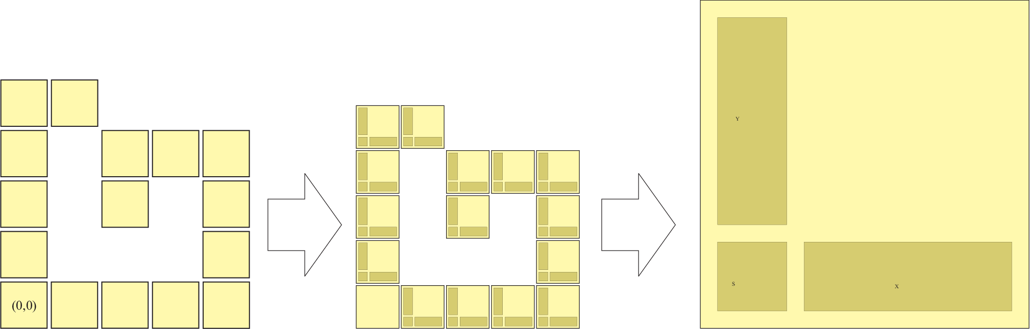
Throughout our discussion, $S_{\vec{u}}$ , $Y_{\vec{u}}$ , and $X_{\vec{u}}$ refer to the square, the vertical rectangle and the horizontal rectangle, respectively, that form the “outer framework” of the set $\left(\left(T_{i}\cup F_{i}\right)+l(i)\cdot\vec{u}\right)$ (See the right-most image in Figure 4).

5.1 Construction Phase 1

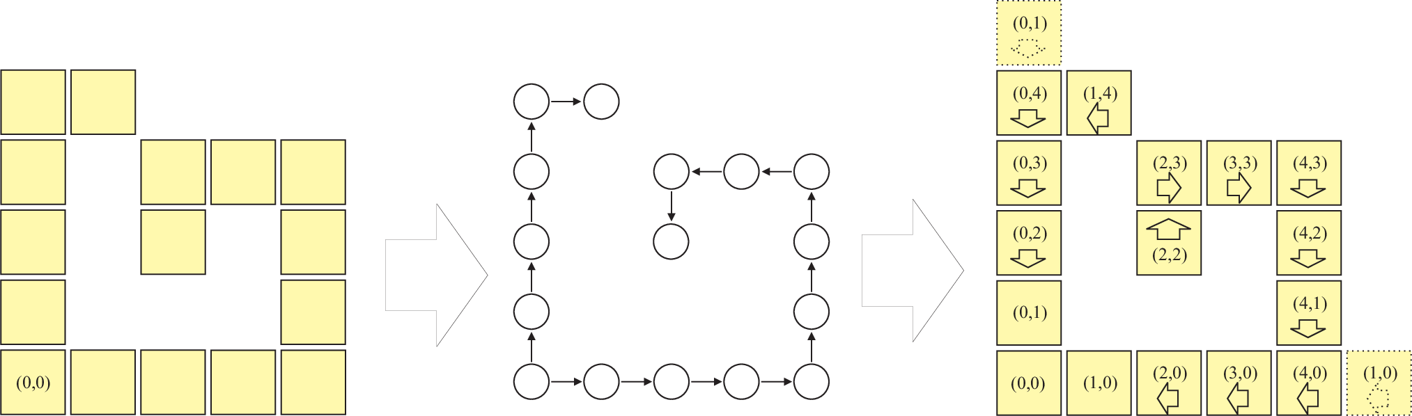
Here, directed graphs are considered. Let $X$ be a nice ( $c$ -discrete) self-similar fractal generated by $V$ . We first compute a directed spanning tree $B=(V,E)$ of $G^{\#}_{V}$ using a breadth-first search, and then compute the graph $B^{\textmd{R}}=\left(V,E^{\textmd{R}}\right)$ , where

E^{\textmd{R}}=\left\{\left(\vec{v},\vec{u}\right)\mid\left(\vec{u},\vec{v}\right)\in E\textmd{ and }\vec{u}\neq(0,0)\right\}\cup\{((0,1),(0,c-1)),((1,0),(c-1),0)\}.

Figure 3 depicts phase 1 of our construction for a particular nice self-similar fractal.

Notation.

For all $\vec{0}\neq\vec{u}\in V$ , $\vec{u}_{\textmd{in}}$ is the unique location $\vec{v}$ satisfying $\left(\vec{u},\vec{v}\right)\in E^{\textmd{R}}$ .

5.2 Construction Phase 2

In the second phase we construct, for each $(0,0)\neq\vec{u}\in V$ , a finite set of tile types $T_{\vec{u}}$ that self-assemble a particular subset of $\mathbf{X}$ . There are two cases to consider.

Case 1: In the first case, we generate, for each $\vec{u}\in V-\left\{(0,0),(0,1),(1,0)\right\}$ , three sets of tile types $T_{S_{\vec{u}}}$ , $T_{X_{\vec{u}}}$ , and $T_{Y_{\vec{u}}}$ that, when combined together, and assuming the presence of $\left(\left(T_{i}\cup F_{i}\right)+l(i)\cdot\vec{u}_{\textmd{in}}\right)$ , self-assemble the set $\left(\left(T_{i}\cup F_{i}\right)+l(i)\cdot\vec{u}\right)$ , for any $i\in\mathbb{N}$ .
Case 2: In the second case, we generate, for each $\vec{u}\in\{(0,1),(1,0)\}$ , the same three sets of tile types ( $T_{S_{\vec{u}}}$ , $T_{X_{\vec{u}}}$ , and $T_{Y_{\vec{u}}}$ ) that self-assemble the set $\left(\left(T_{i}\cup F_{i}\right)+l(i)\cdot\vec{u}\right)$ “on top of” the set $\left(\left(T_{i-1}\cup F_{i-1}\right)+l(i-1)\cdot\vec{u}_{\textmd{in}}\right)$ , for any $i\in\mathbb{N}$ .

Finally, we let $T_{\mathbf{X}}=\bigcup_{(0,0)\neq\vec{u}\in V}{T_{\vec{u}}}$ , where $T_{\vec{u}}=T_{S_{\vec{u}}}\cup T_{X_{\vec{u}}}\cup T_{Y_{\vec{u}}}$ . Figure 4 gives a visual interpretation of the second phase of our construction. Our TAS is $\mathcal{T}_{\mathbf{X}}=(T_{\mathbf{X}},\sigma,2)$ , where $\sigma$ consists of a single “seed” tile type placed at the origin. Our full construction yields a tile set of 5983 tile types for the fractal generated by the points in the left-most image in Figure 4.

5.3 Details of Construction

Note that in our construction, the self-assembly of the sub-structures $S_{\vec{u}}$ , $Y_{\vec{u}}$ , and $X_{\vec{u}}$ can proceed either forward (away from the axes) or backward (toward the axes).

5.3.1 Forward Growth

We now discuss the self-assembly of the set $((T_{i}\cup F_{i})+\vec{u}\cdot l(i))$ for $\vec{u}\in V$ satisfying $\vec{u}_{\textmd{in}}\in\left(\vec{u}+\{(-1,0),(0,-1)\}\right)$ .

If $\vec{u}\not\in\{(0,0),(0,1),(1,0)\}$ (i.e., case 1 of phase 2), then the tile set $T_{S_{\vec{u}}}$ self-assembles the square $S_{\vec{u}}$ directly on top (or to the right) of, and having the same width (height) as, the rectangle $Y_{\vec{u}_{\textmd{in}}}$ ( $X_{\vec{u}_{\textmd{in}}}$ ). If $\vec{u}\in\{(0,1),(1,0)\}$ (i.e., case 2 of phase 2), then the tile set $T_{S_{\vec{u}}}$ self-assembles the square $S_{\vec{u}}$ on top (or to the right) of the set $Y_{\vec{u}_{\textmd{in}}}$ such that right (top) edge of the former is flush with that of the latter. Note that in case 2, the width of $Y_{\vec{u}_{\textmd{in}}}$ is always one less than that of $S_{\vec{u}}$ . In either case, it is straightforward to construct such a tile set $T_{S_{\vec{u}}}$ .

The tile set of $T_{Y_{\vec{u}}}$ self-assembles a fixed-width base- $c$ counter (based on the “optimal” binary counter presented in [4]) that, assuming a width of $i\in\mathbb{N}$ , implements the following counting scheme: Count each positive integer $j$ , satisfying $1\leq j\leq c^{i}-1$ , in order but count each number exactly

[\![c\textmd{ divides }j]\!]\cdot\rho(j)+[\![c\textmd{ does not divide }j]\!]\cdot 1

times, where $\rho(j)$ is the largest number of consecutive least-significant 0’s in the base- $c$ representation of $j$ , and $[\![\phi]\!]$ is the Boolean value of the statement $\phi$ . The value of a row is the number that it represents. We refer to any row whose value is a multiple of $c$ as a spacing row. All other rows are count rows. The type of the counter that self-assembles $Y_{\vec{u}}$ is $\vec{u}$ .

Each counter self-assembles on top (or to the right) of the square $S_{\vec{u}}$ , with the width of the counter being determined by that of the square. It is easy to verify that if the width of $S_{\vec{u}}$ is $i+2$ , then $T_{\vec{Y}_{\vec{u}}}$ self-assembles a rectangle having a width of $i+2$ and a height of

\left(c^{2}+1\right)c^{i}+\frac{c^{i}-1}{c-1}=l(i)-(i+2),

which is exactly $Y_{\vec{u}}$ . Figure 5 shows the counting scheme of a base- $3$ counter of width $3$ . We construct the set $T_{X_{\vec{u}}}$ by simply reflecting the tile types in $T_{Y_{\vec{u}}}$ about the line $y=x$ , whence the three sets of tile types $T_{S_{\vec{u}}}$ , $T_{X_{\vec{u}}}$ , and $T_{Y_{\vec{u}}}$ self-assemble the “outer framework” of the set $((T_{i}\cup F_{i})+\vec{u}\cdot l(i))$ .

The “internal structure” of the set $((T_{i}\cup F_{i})+\vec{u}\cdot l(i))$ self-assembles as follows. Oppositely oriented counters attach to the right side of each contiguous group of spacing rows in the counter (of type $\vec{u}$ ) that self-assembles $Y_{\vec{u}}$ . The number of such spacing rows determines the height of the horizontal counter, and its type is $\left(0,j/c\mod c\right)$ , where $j$ is the value of the spacing rows to which it attaches. We also hard code the glues along the right side of each non-spacing row to self-assemble the internal structure of the points in the set $T_{0}$ .

The situation for $X_{\vec{u}}$ is similar (i.e., a reflection of its vertical counterpart), with the exception that the glues along the top of each non-spacing row are configured differently than they were for $Y_{\vec{u}}$ . This is because nice self-similar fractals need not be symmetric.

One can prove that, by recursively attaching smaller oppositely-oriented counters (of the appropriate type) to larger counters in the above manner, the internal structure of $((T_{i}\cup F_{i})+\vec{u}\cdot l(i))$ self-assembles.

5.3.2 Reverse Growth

We now discuss the self-assembly of the set $((T_{i}\cup F_{i})+\vec{u}\cdot l(i))$ , for all $\vec{u}\in V$ satisfying $\vec{u}_{\textmd{in}}\in\left(\vec{u}+\{(1,0),(0,1)\}\right)$ .

In this case, the tile set $T_{Y_{\vec{u}}}$ ( $T_{X_{\vec{u}}}$ ) self-assembles the set $Y_{\vec{u}}$ ( $X_{\vec{u}}$ ) directly below (or to the left of) the square $S_{\vec{u}_{\textmd{in}}}$ , and grows toward the $x$ -axis (or $y$ -axis) according to the base- $c$ counting scheme outlined above. We also configure $T_{Y_{\vec{u}}}$ ( $T_{X_{\vec{u}}}$ ) so that the right (or top)-most edge of $Y_{\vec{u}}$ ( $X_{\vec{u}}$ ) is essentially the “mirror” image of its forward growing counterpart (See Figure 6). This last step ensures that the internal structure of $((T_{i}\cup F_{i})+\vec{u}\cdot l(i))$ self-assembles correctly. Next, the square $S_{\vec{u}}$ attaches to the bottom (or left)-most edge of $Y_{\vec{u}}$ ( $X_{\vec{u}}$ ). Finally, the set $X_{\vec{u}}$ ( $Y_{\vec{u}}$ ) self-assembles via forward growth from the left (or top) of the square $S_{\vec{u}}$ .

5.3.3 Proof of Correctness

To prove the correctness of our construction, we use a local determinism argument. The details of the proof are technical, and therefore omitted from this version of the paper.

6 Conclusion

In this paper, we (1) established two new absolute limitations of the TAM, and (2) showed that fibered versions of “nice” self-similar fractals strictly self-assemble. Our impossibility results motivate the following question: Is there a discrete self-similar fractal $X\subsetneq\mathbb{N}^{2}$ that strictly self-assembles in the TAM? Moreover, our positive result leads us to ask: If $X\subsetneq\mathbb{N}^{2}$ is a discrete self-similar fractal, then is it always the case that $X$ has a “fibered” version $\mathbf{X}$ that strictly self-assembles, and that is similar to $X$ in some reasonable sense?

Acknowledgment

We thank Dave Doty, Jim Lathrop, Jack Lutz, and Aaron Sterling for useful discussions.

References

[1] Leonard M. Adleman, Qi Cheng, Ashish Goel, Ming-Deh A. Huang, David Kempe, Pablo Moisset de Espanés, and Paul W. K. Rothemund, Combinatorial optimization problems in self-assembly, Proceedings of the Thirty-Fourth Annual ACM Symposium on Theory of Computing, 2002, pp. 23–32.
[2] Gagan Aggarwal, Michael H. Goldwasser, Ming-Yang Kau, and Robert T. Schweller, Complexities for generalized models of self-assembly, Proceedings of ACM-SIAM Symposium on Discrete Algorithms, 2004.
[3] T. M. Apostol, Modular functions and Dirichlet series in number theory, Graduate Texts in Mathematics, vol. 41, Springer-Verlag, 1997.
[4] Qi Cheng, Ashish Goel, and Pablo Moisset de Espanés, Optimal self-assembly of counters at temperature two, Proceedings of the First Conference on Foundations of Nanoscience: Self-assembled Architectures and Devices, 2004.
[5] D. Doty, X. Gu, J.H. Lutz, E. Mayordomo, and P. Moser, Zeta-Dimension, Proceedings of the Thirtieth International Symposium on Mathematical Foundations of Computer Science, Springer-Verlag, 2005, pp. 283–294.
[6] L. Euler, Variae observationes circa series infinitas, Commentarii Academiae Scientiarum Imperialis Petropolitanae 9 (1737), 160–188.
[7] G. Hardy and E. Wright, An introduction to the theory of numbers, 5th ed., Clarendon Press, 1979.
[8] Ming-Yang Kao and Robert Schweller, Reducing tile complexity for self-assembly through temperature programming, Proceedings of the 17th Annual ACM-SIAM Symposium on Discrete Algorithms (SODA 2006), Miami, Florida, Jan. 2006, pp. 571-580, 2007.
[9] James I. Lathrop, Jack H. Lutz, Matthew J. Patitz, and Scott M. Summers, Computability and complexity in self-assembly, Proceedings of The Fourth Conference on Computability in Europe (Athens, Greece, June 15-20, 2008). To appear., 2008.
[10] James I. Lathrop, Jack H. Lutz, and Scott M. Summers, Strict self-assembly of discrete Sierpinski triangles, Proceedings of The Third Conference on Computability in Europe (Siena, Italy, June 18-23, 2007), 2007.
[11] Urmi Majumder, Thomas H LaBean, and John H Reif, Activatable tiles for compact error-resilient directional assembly, 13th International Meeting on DNA Computing (DNA 13), Memphis, Tennessee, June 4-8, 2007.
[12] Paul W. K. Rothemund, Theory and experiments in algorithmic self-assembly, Ph.D. thesis, University of Southern California, December 2001.
[13] Paul W. K. Rothemund and Erik Winfree, The program-size complexity of self-assembled squares (extended abstract), Proceedings of the Thirty-Second Annual ACM Symposium on Theory of Computing, 2000, pp. 459–468.
[14] N.C. Seeman, Nucleic-acid junctions and lattices, Journal of Theoretical Biology 99 (1982), 237–247.
[15] David Soloveichik and Erik Winfree, Complexity of self-assembled shapes, SIAM Journal on Computing 36, 2007, pp. 1544–1569.
[16] Hao Wang, Proving theorems by pattern recognition – II, The Bell System Technical Journal XL (1961), no. 1, 1–41.
[17] , Dominoes and the AEA case of the decision problem, Proceedings of the Symposium on Mathematical Theory of Automata (New York, 1962), Polytechnic Press of Polytechnic Inst. of Brooklyn, Brooklyn, N.Y., 1963, pp. 23–55.
[18] Erik Winfree, Algorithmic self-assembly of DNA, Ph.D. thesis, California Institute of Technology, June 1998.