Gravitational Lensing Constraints on Dynamical and Coupled Dark Energy
Abstract
Upcoming Weak Lensing (WL) surveys can be used to constrain Dark Energy (DE) properties, namely if tomographic techniques are used to improve their sensitivity. In this work, we use a Fisher matrix technique to compare the power of CMB anisotropy and polarization data with tomographic WL data, in constraining DE parameters. Adding WL data to available CMB data improves the detection of all cosmological parameters, but the impact is really strong when DE–DM coupling is considered, as WL tomography can then succeed to reduce the errors on some parameters by factors
1 Introduction
The first data system requiring Dark Energy (DE) concerned cosmic acceleration, detected through high-redshift supernovae [1]. CMB [2] and deep sample [3] data supported also the DE case, showing that the density parameter for non–relativistic matter , while the total density parameter
In the most popular scenario, DE is ascribed to a cosmological constant . Alternative options include a self–interacting scalar field, (quintessence or dynamical DE [4, 5]) and modifications of General Relativity [6].
It is known that models with (CDM) apparently accommodate all available data systems. The problem is the physical origin of which can be a false vacuum; this however causes well known fine tuning and coincidence problems.
The former problem is partially eased in dynamical DE (dDE) scenarios, when self interaction is due to a tracking potential [7]. If is SUGRA [5] , the fit with data is at least as good as for CDM [8].
In the attempt to ease the coincidence problem, DM–DE interaction (e.g., [9, 10]) was also considered, yielding an energy transfer between the dark components, so allowing a (quasi)–parallel scaling of DM and DE from a fairly high redshift until the present. While laboratory data set no significant constraint on DM–DE interaction strength, parametrized by (see below), recent works placed constraints on possible couplings, by using SNIa data [11] or the redshift evolution of the Hubble parameter, [12]. Accordingly, –0.15 [13, 14] is hardly consistent with observations.
Unfortunately, such a low coupling level no longer eases the coincidence problem [15], but, once the genie has come out from the lamp, it is hard to put it back inside. The point is whether low values of , as allowed by current data, can interfere with future data analysis. In particular, when we allow for non–zero , how do errors on other parameters behave?
In this work we tried to answer this question by using a Fisher matrix technique. We considered two different models, set by similar values of cosmological parameters, without and with coupling. In the latter case, we took Starting from these models, we evaluated the expected errors on cosmological parameters, as obtained when data concern just CMB anisotropy and polarization or include tomographic weak lensing (WL).
As a matter of fact, in coupled models, the time evolution of the dark components is non–standard. If such models are considered in a Newtonian approximation, it is as though DM particles had a –dependent mass. Also for quite low ’s, this anomalous scaling leaves an imprint on both the expansion history of the Universe, and the growth of (matter) fluctuations, at the linear and non–linear levels (e.g. [16]).
However, any detected evolution of can be reproduced through a suitable redshift dependence of DE density and state parameter , when approaches (the Planck mass). A risk is that, if matter and dark energy are coupled, fitting observations leads to an estimate of a phantom equation of state (), even if at all redshifts [17].
In principle, this risk can be excluded if the redshift dependence of the growth factor is also tested, through the increase in number and concentration of bound systems. Data providing information both on and are therefore able to discriminate between coupled and uncoupled models. Experiments, or combinations of experiments, probing and are then needed.
CMB data, used to constrain coupling [13, 18], place only upper limits on . The analysis of Ly– and the matter power spectrum of the 2dF and SDSS surveys [14] does not lead to great improvements. At the available sensitivity level, such data systems provide just weighted integrals of and , which remain consistent with a rather wide set of options.
On the contrary, gravitational lensing, alone or in combination with CMB data, was already shown to be a powerful tool for the analysis of DE. WL tomography probes the power spectrum at different redshifts and is thus well suited to constrain
In this work we aim to put these conceptual points on a more quantitative basis and to deepen the case of coupling, by performing a Fisher analysis of future WL surveys and CMB experiments.
2 Models and definitions
2.1 Interacting Dark Energy
We consider a cosmological model where the DE field interacts with the cold DM component. The model requires the specification of the potential and the function characterizing the coupling. The equation of motion for then reads
| (1) |
Here dots denote ordinary time differentiation, and is DM energy density. In turn, its evolution is governed by
| (2) |
This equation can be integrated and gives:
| (3) |
For eqs. (1), (3) return ordinary dDE equations. The equations for the other components remain unchanged. In a generic coupled model, then, the ratio between the energy densities of cold DM and baryons is not fixed, but evolves in time according to .
However, it is always possible to define an effective DE component of density
| (4) |
In general, is not guaranteed to be positive and detecting would be a clear indication that our description of the dark sector is not adequate. Lacking such clear giveaway, however, experiments probing can hardly discriminate between DE–DM interaction and an ad hoc DE component. If its effective state parameter is , data may appear to require phantom DE (see [19] for discussion).
Coupling affects also fluctuation growth. In the Newtonian limit, i.e. well below the horizon, and neglecting the contribution of radiation, baryons and DM fluctuations grow according to the equations (e.g. [16, 20]):
where we defined so that
| (8) |
while . Therefore, baryons and DM perturbations grow at different rates and, even soon after recombination, a growing mode no longer exists (see Fig. 1), leading to a bias between baryon and DM perturbations. Analytical models of spherical collapse have shown that this differential growth results in a baryon–DM segregation, with baryons occupying the outer regions of collapsed objects [21].
Eqs (2.1) also show that the growth equations explicitly depend on both and ; therefore, if we measure the growth from data, a possible anomalous scaling can no longer be masked though an ad–hoc definition of an effective DE density. It is then licit to conclude that experiments probing the rate of growth of fluctuations are in principle well suited to test coupling between the dark components.

In this work we are interested to combining WL and CMB data, which cannot be accurately described using current parametrisations [22]. Therefore, we follow a more conventional approach and choose the functional forms
| (9) |
The SUGRA [5] potential depends on the slope and the energy scale . Fixing DE density today and (), however, determines a unique value of (). CMB, SNIa and deep sample data yield GeV [8], in the absence of coupling. Here we focus on the SUGRA potential as it naturally arises in the context of Supergravity Theories and is an example of tracking potential characterized by a rapid time variation of the equation of state, when DE becomes dominant. Therefore, assuming a constant for this class of potential may lead to misleading results. Different choices for the potential are clearly possible.
The coupling function depends on , and is the field value today. In this work we assume a constant (see however [19] for a different approach); data place the upper limit [13, 14]. For reasonable values of the cosmological parameters and of , we expect coupling effects not to be relevant for , so that the dynamically interesting values for the coupling lies in the range .
2.2 Weak lensing
Among the cosmological probes allowing the analysis of the nature of DE, the cosmological WL has been earning a fundamental role (see [23, 24, 25, 26] for a thorough review). In fact, next generation WL surveys will cover a significant fraction of the sky and observe galaxies at deeper redshift, making WL a powerful tool to study the properties of the Universe. Furthermore, WL tomography will allow to significantly increase the cosmological information that can be recovered from such surveys (see [27] and [28, 29, 30] for details about lensing tomography).
The power spectrum for the WL convergence between the th– and th– redshift bin is given by:
| (10) |
Here is the non–linear matter power spectrum, at the redshift and wave number ; the quantity is the radial comoving distance between and ,
| (11) |
while
| (12) |
is the window function which weights different redshift bins according to the factor ,
| (13) |
being the i–th redshift bin. The function is the normalized redshift distribution of the source galaxies falling in the -th photometric redshift bin, per unit solid angle,
| (14) |
where
| (15) |
The last expression codifies the effect of errors in photometric redshifts of source galaxies [31]. In fact, due to the large number of observed galaxies with future surveys, one needs to refer to their photometric redshifts, even if the determination of these redshifts may be not so accurate as the spectroscopic ones. In the model given by (15), the mapping between the photometric and the spectroscopic redshift is obtained convolving the overall galaxy distribution per unit solid angle, , with a probability distribution in at a given . We choose a Gaussian function at each redshift for the distribution of photometric redshifts, i.e.
| (16) |
while the overall distribution of source galaxies is chosen to have the parametrized form:
| (17) |
where , and are the parameters. One can easily check that equation (15) turns into:
| (18) |
with and the error function.
The cosmic shear power spectrum will receive a shot-noise contribution from the random intrinsic ellipticities of source galaxies and measurement error [32]. Thus, the observed power spectrum between redshift bins and can be expressed as:
| (19) |
where is the rms shear due to intrinsic ellipticity and measurement noise (we assume [27]) and
| (20) |
is the average number density of galaxies per steradians in the -th redshift bin, being the number of galaxies per square arcminute and the fraction of sources belonging to the bin.
The covariance between the power spectra and is approximately given by
| (21) |
where is the sky fraction covered by the survey and is the bin width centred at . The above expression assumes that the power spectrum in each multipole bin is very flat, in order to replace the value of the spectrum evaluated at the bin center with the average of spectrum over each bin (see A for the complete expression). In addition, we have not included the non-Gaussian term, due to the contribution of the shear trispectrum [33, 34].
2.3 Fisher’s formalism
The Fisher matrix formalism [35, 36, 37] provides lower limits to the error bars of the cosmological parameters one wishes to measure. The basic tool in Fisher’s method is the likelihood function, yielding the probability that a model gives the set of data x.
Suppose we want to test an hypothesis, i.e. a cosmological model set by parameters . The likelihood function is often a complicated function of ; the value corresponding to the peak of defines the maximum likelihood estimator which, in the limit of large data sets, becomes the best unbiased estimator of the actual parameter set. Thus, the likelihood can be Taylor expanded to second order (the first non–vanishing term) around , being so approximated with a multivariate Gaussian distribution
| (22) |
here
| (23) |
is a positive semi-definite non-singular matrix, dubbed covariance matrix of the . We remind that Equation (22) holds just in a sufficiently small neighborhood around the maximum . In turn, the Fisher information matrix reads
| (24) |
the average is taken over all possible data realizations, given the model parameters. The feature making Fisher’s formalism so significant is the Cramér-Rao theorem. It states that the parameter variance about any unbiased estimator value owns a lower bound: , if the other parameters are estimated from the data as well, , if all the other parameters are known. Therefore,the Fisher information matrix components are the expectation values of . Accordingly, the inverse of the Fisher matrix is an estimate of the covariance matrix of the parameters .
A convenient way to re–write the Fisher matrix is computing the derivatives of the likelihood function using the following chain rule [38]:
| (25) |
Thus, the Fisher matrix (24) can be expressed as:
| (26) | |||||
| (27) | |||||
| (28) |
where and , respectively, are the Fisher and the covariance matrix for the observables x. The region in the –dimensional space of the parameters, defined by , is a hyper–ellipsoid of constant probability density for the function (22). Marginalizing over the other parameters, one can project this ellipsoid in the two–parameter subspace, yielding a two–dimensional ellipse. The analytical expression for the projected ellipse for the two parameters and is given by [39]:
This can be interpreted as an estimate of the confidence region within a given confidence level for the two parameters and .
3 Forecasts for Future Experiments
We present here the results of the Fisher analysis of future experiments, considering both WL and CMB measurements. For definiteness we assume a fiducial WL survey with characteristics similar to those of the recently proposed DUNE project [40]. We assume a redshift distribution of the form (17) with , and , corresponding to a median redshift of the survey (see [27]), and a mean surface density of galaxies . The full survey, covering half of the sky (), is divided into redshift bins, with given by equation (16) and .
We consider lensing multipoles up to , since we find that results do not depend significantly on larger . However, one should bear in mind that when considering scales there could be some non–linear and baryonic effects on the matter power spectrum, and so on the WL spectrum [41]. These effects, not yet well understood, could be important for forecasts. However, in this work we suppose these effects to be negligible.
For CMB data, we consider an ideal experiment with characteristics based on the 143GHz PLANCK channel: angular resolution and sensitivity , .
The cosmological model we consider is characterized by 7 parameters with fiducial values:
Here represents the current total (CDM + baryons) matter density in units of the critical density; and are the physical baryons and total matter densities, respectively; is the slope of the primordial power–law spectral index of density fluctuations; is the rms mass fluctuation in spheres of 8 Mpc radius while and were defined in Sec. 2.1. Let us notice that the class of DE models considered here reduces to CDM for and . Moreover, the fiducial values of DE parameters and are chosen in order to reproduce at an effective equation of state which mimics the case of CDM model, . Finally, when dealing with CMB data, we also need to fix the value of the optical depth to reionization, .
We compute the CMB anisotropies (temperature and polarisation) power spectra and the transfer functions, used to calculate linear matter power spectrum, using a modified version of CAMB [42]. To evaluate the non–linear matter power spectrum, , we employ the prescription by Smith et al. [43]. This is only tested for model with a cosmological constant; as we are concerned here with Fisher matrix estimates assume that the results of [43] can be extended to coupled models simply by taking into account the non–standard scaling of (eq. 3). Numerical derivatives were evaluated considering a stepsize, except for , where we adopted a stepsize on .
3.1 CMB measurements
| CMB | WL | WL+CMB | ||||
|---|---|---|---|---|---|---|
| SUGRA | SUGRA | SUGRA | SUGRA | SUGRA | SUGRA | |
| 100 | 0.016 | 0.019 | 0.5 | 0.9 | 0.011 | 0.012 |
| 0.002 | 0.006 | 0.016 | 0.03 | 0.0004 | 0.0005 | |
| 0.05 | 0.12 | 0.002 | 0.0014 | 0.0011 | 0.0014 | |
| 0.004 | 0.005 | 0.012 | 0.018 | 0.0014 | 0.0021 | |
| 0.07 | 0.13 | 0.0026 | 0.0029 | 0.0017 | 0.0016 | |
| 7.2 | 9.5 | 0.89 | 1.1 | 0.28 | 0.28 | |
| – | 0.04 | – | 0.018 | – | 0.0016 | |
| 0.005 | 0.006 | – | – | – | – | |
Table 1 lists the estimated errors on the various parameters considered. For each data set, we compare forecasts for the target model with results for a SUGRA model with the same values of the relevant parameters. The table clearly shows that a PLANCK–like experiment is able to provide a measurement of a direct DE–DM interaction at 68% confidence level, even for moderate values of the coupling strength . However, we expect that at 90% confidence level data will still be compatible with .
In any case, allowing for a direct interaction strongly degrades the experimental sensitivity on the parameters characterizing the matter density and the normalization of the primordial spectrum of density fluctuations. Errors on these quantities increase by a significant amount.
Figure 2 shows the joint confidence regions between and each of the other parameters, except for , considering only CMB data. In each plot we marginalized over the parameters not shown. is strongly correlated with most parameters considered here, with the exception of (and ), thus introducing additional degeneracies in actual data analysis.
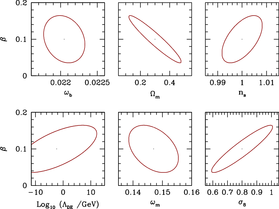
A detailed characterization of these degeneracies would require a different approach than that followed here (e.g. Monte Carlo Markov Chains simulations). We just point out that they can be understood recalling that the heights of the acoustic peaks of CMB spectra are sensitive to the total matter density and to baryon/dark matter ratio at last scattering. In coupled models, these quantities are not univocally determined by their present day value, but strongly depend on . In addition, the total growth between the last scattering epoch and today is strongly sensitive to , resulting in a clear degeneracy between and .
Let us notice that, as we are concerned with a combination of CMB and WL data, the parameter set is not optimized for CMB experiments. Using a different parametrisation can alter error estimates and/or the degeneracies between the various parameters. In particular, CMB data are better described in terms of the angle subtended by the acoustic horizon at recombination, , and the amplitude of the primordial spectrum of density fluctuations , rather than in terms of and . This results in large errors on the latter parameters, when CMB data alone are considered. Adopting a set of parameters better suited to the analysis of CMB data results in slightly lower error estimates overall, but the effects of coupling are largely unchanged.
3.2 Weak Lensing


Figure 3 is analogous to figure 2 for our target weak lensing survey. Together with Table 1, these results show the great potential of WL surveys in constraining interacting DE models. Marginalized errors on and are of the order of and ; these figures represent a factor of 2, or more, improvement over Planck estimates. WL data alone can clearly distinguish the target model from a non–coupled model or a cosmological constant even at the 3-level, viceversa assuming a reference SUGRA model with , we can expect to put an upper limit , at the same confidence level (see figure 4).
As expected, WL surveys perform significantly better than CMB experiments also with respect to parameters specifying the current matter density, and . Moreover, constraints on these parameters are not significantly affected by the coupling degrees of freedom. Errors on the remaining parameters, instead, increase by a factor of . Finally, we consider a combination of CMB and WL data. CMB and WL probe very different epoch of the Universe and are sensitive to different combination of cosmological parameters. Considering both CMB and WL data allows to constrain the DE parameters with a few percent accuracy, and significantly reduces the degeneracies introduced by DE coupling. In this case, the errors on the cosmological parameters are very similar in both models considered, with the exception of .
Next we considered how our results depend on the characteristic assumed for the target survey. In figure 5 the impact of mean surface density of galaxies on the determination of and . With constraints on degrades by , while gives only a marginal improvement on expected errors; constraints on are similarly affected. However, even in the worst case considered here, next generations WL survey will provide an improvement over the information that we are likely to obtain from PLANCK data.
Lastly, we consider the dependence of our results on the number of bins and the multipoles range considered. In figure 6 we plot the inverse of the expected variance on and as a function of the maximum multipole considered in the analysis and for different number of bins. With 3 redshift bins, the precision on both parameters depends mostly on multipole up to a few thousands; smaller scales do not provide a significant contribution. Dividing the survey in 5 bins strongly improves the constraints on both parameters and allows to exploit information from multipoles up to . For a DUNE–like survey, a further increase in the number of bins does not lead to significant improvements on the constrains on coupled models parameters.
It must be outlined that these results assume that the theoretical framework used to predict the matter power spectrum on intermediate () and small () scales can accurately account for the effects of baryons on non–linear structures. In general, the fitting formulas used to predict the non–linear power spectrum are calibrated using dissipationless N–body simulations and, therefore, do not properly describe baryonic structures. While baryons make up of the matter in the Universe and on large scales are expected to trace the DM field, their distribution inside halos is significantly different from DM. In turn, this alters the shape of the non–linear power spectrum on the corresponding scales, and the possibility of extracting precision constraints from hinges on our capability of accurately modeling baryon physics [41]. However, simulations do not yet have the accuracy required for precision constraints and the problem is even more serious for the coupled models considered in this work. Modelling non linear stages though spherical growth, Mainini [44] shew that baryons and DM will be however differently distributed, even independently of the onset of gas dynamics. N–body simulations of cDE models were performed [45], by using a Ratra–Peebles [46] potential; hydro simulations, instead, were never produced. Should accurate prediction be still unavailable for the analysis of a DUNE–like experiment, a more conservative cutoff of would be required. Figure 6 shows that in this case the expected errors on and would increase by a factor .
4 Discussion
All previous analysis shows that, even if we admit quite a little DM–DE coupling, we open a Pandora’s box, leading to a severe degradation in our capacity to deduce cosmological parameters from a given set of measures.
As a matter of fact, coupling destroys our trust that the period between the recombination and the start of DE relevance is under control. If coupling is absent, during such period SCDM is a fair approximation. Let us then remind what happens to the growth factor, as soon as coupling is onset: Figure 1 shows that: (i) deviations from SCDM are significant already when ; (ii) they are then different for DM and baryons; (iii) they work in the opposite direction, in respect to the effects of a DE components.
As far as the growth factor is concerned, a tiny coupling is able to overwhelm a huge DE amount, with compensation occurring for –0.4 , however keeping always at values greater by –15. Altogether, growth is faster in coupled models. Hence, if we do not include the information that coupling is zero in the fit, we can find an agreement between data and a wider range of DE amounts.

Similar points can be made for the comoving radial distance (see eq. 11). In Figure 7 we compare comoving distances for CDM with various cosmologies. The Figure shows that dDE, in the absence of other parameter shifts, sets the Last Scattering Band (LSB) closer to the observer. Once again, a mild coupling acts in the opposite direction and tends to re-set the LSB at the distance it had in . In the Figure we consider the behavior of distances also for a rather strong coupling, . Then the distance behavior is different in the period when DE density can be neglected, in respect to the epoch when DE and DM have similar densities. The key point, however, is that the LSB becomes then farther from the observer. When fitting CMB data to such models, in order to compensate such effect, the value of tends to be increased. Strong coupling therefore yields a large Hubble parameter estimate.
Figures 8 finally show the scale dependence of the density parameters in the different models. Once again, when DE is mildly coupled, a behavior more similar to is recovered. On the contrary, when considering a greater coupling strength, we see that DE and DM keep similar densities up to a fairly large redshift. This was indeed the initial motivation of cDE cosmologies.


Altogether, these Figures indicate that adding a small coupling reduces the effects of the very passage from to dDE; owing to the excellent fit that cosmologies have with data, this tells us that only highly refined CMB data will be able to test the possibility that a mild DM–DE coupling exists.
On the contrary, a stronger coupling, although easing the coincidence problem, displaces several observables in a unacceptable way.
5 Summary and Conclusions

Future WL surveys will certainly put more stringent constraints on cosmological parameters and will be crucial to break quite a few degeneracies between parameters.
Within this context, in this paper we focus on coupled DE models with a twofold aim. Detecting a signal of DM–DE coupling would be certainly decisive to fix the nature of the dark components. Henceforth determining the level of sensitivity needed to appreciate such an effect is crucial in setting the appeal of forthcoming projects. There is however a complementary aspect which deserves much attention. In order to convert raw data into physical information, a set of parameters, spanning a variety of models, is to be fixed; a bias on parameter selection, however, can lead to an optimistic estimate of the confidence level for the best fitting model, far from reality.
In this paper, we focused on this kind of danger, when we open the option of DM–DE coupling. Even if such coupling is absent or quite weak, we showed that just considering its possibility may widen the error bars for a number of parameters, also apparently unrelated to the coupling itself. In a sense, when a new degree of freedom is opened, such an effect is natural and expected. Coupling, however, has really a major impact, affecting different parameters for the different observables considered here; moreover, its impact is drastically reduced when we work out parameter values by using simultaneously both observables.
Before outlining our main conclusions it is however worth reminding a technical limit we had to face. While CMB predictions depend on linear spectra, the WL spectrum is limited to its non–linear shape. For the purpose of the present analysis, we assumed that prescription for CDM models [43] can be trivially extrapolated to coupled models, so enabling us to estimate the non linear spectrum once the linear spectrum is known. Let us however remark that the shift was estimated from quite a wide set of CDM simulations. Simulations of cosmological models with state parameters , although performed by several authors, are still not so extensively studied as CDM; let alone coupled DE simulations: in this case the only available simulations are due to [45] and deal with a potential different from SUGRA.
However, differences between prescriptions for CDM and dDE are small [47] and it seems however clear that model differences can most affect the rate of evolution of halo concentration, slightly shifting the scale where non–linearity effects become significant. The use of more precise prescriptions can therefore only cause minor variation on the estimated errors and, although welcome, such simulations are not expected to interfere substantially with our conclusions.
Our estimates were based on assuming that a photometric survey is available, with and a median redshift , covering half of the sky (). These features are similar to the recently proposed DUNE experiment [40]. We also compared and combined results from WL with the constraints expected for an ideal Planck–like experiment. The basic results of our calculations are quoted in table 1 which is one of the main results of this work.
A first set of conclusions concerns an ideal CMB experiment considered by itself. In this case, introducing coupling degrees of freedom is crucial for the error estimates on some of parameters, also apparently unrelated to coupling. In particular, while the error on keeps 1%, the errors on and increase from 1.3% to 3.9% and from 9% to 16%, respectively.
From a physical point of view, the option opened by coupling is that expansion rate and fluctuation growth, from the last scattering band to the observer’s site, is non–standard (e.g., the proportionality law could be mildly violated). Although CMB data themselves set stringent limits on such deviations, this widens the volume of the parameter space consistent with a given data set; in particular, it increases the likelihood of values of that would otherwise be negligible and, because of the intercorrelation amongst parameters, this reflects immediately on and estimates.
Similar effects occur in WL experiments, although involving different parameters. Such experiments are a direct test of , whose estimated error is reduced by a factor in respect to a CMB experiment. When the coupling option is opened, the error on does not increase; on the contrary, it becomes easier to attribute raw data uncertainties to other parameters and, although marginally, the error on becomes somehow smaller.
A completely new situation occurs if both CMB and WL measurements are simultaneously used. In this case, the opening of the coupling option causes just a marginal increase of the errors on most parameters. This is a clear indication of the complementarity of the CMB and WL measurements, as described in [48] and one of our conclusion is that the combination of these observables, besides of providing parameter values independent of , can set a (nearly–)final word on the coupling option.
As a matter of fact, by comparing figure 2, figure 3 and figure 9, we see that, when joining CMB and WL results, the degeneracies, between and , as well as between and , disappear. Breaking degeneracies is the main aim when different observables are simultaneously considered. We see that, from this point of view, the efficiency of using both CMB and WL measures can be hardly overestimated.
Let us then focus on the case of the spectral index of scalar fluctuations. When both CMB and WL data are used to constrain , a sharp reduction of errors occurs. No surprise that CMB data, by themselves, reflecting the state of the universe before the onset of non linear processes, were more efficient to constrain , with or without coupling, than WL measures. Joining together the two observables, we then see errors to decrease from 0.4% and 1.2% down to 0.16%, in the uncoupled case; in the presence of coupling we have a similar behavior, with errors passing from 0.5% and 1.8% down to 0.25%. The error level achieved, in both cases, is exceptional, even for precision cosmology, and clearly suggests to relieve the constraint of a single value, so inspecting its possible scale dependence, with realistic possibilities to find a direct insight into the nature of the inflationary potential.
In conclusion, future WL surveys could really allow a significant step forward in the comprehension of the dark cosmic side; we can adfirm that, when they will be available, the endeavour to put the genie back inside the lamp will approach a full success.
Appendix A Convergence power spectrum covariance
In order to determine the convergence power spectrum covariance, one can introduce the so called “flat-sky” approximation and treat the sky as flat, replacing spherical harmonic sums with Fourier transforms (FT). Of course, this approximation is acceptable just for small angular scales We also consider the tomographic case and use Greek letters as superscripts to denote quantities belonging to different redshift bins. The FT of the convergence field can be defined as:
| (35) |
while the convergence power spectrum and trispectrum are, respectively:
| (36) |
| (37) |
here is the Dirac function. The value of the lensing power spectrum in correspondence of a multipole can be estimated as the mean over a multipole bin of width , centered at :
| (38) |
where is the area of the shell of width corresponding to , while is the area of the survey. Quite in the same way, for the trispectrum we have:
| (39) |
Let us then consider the following expression:
| (40) |
The 4-point function at the r.h.s. can be decomposed in its connected parts:
| (41) |
Replacing their expression in eq. (40), one can easily recognize the contribution of the trispectrum, using eq. (37):
| (42) | |||
| (43) |
where . Owing to the definition of covariance,
| (44) |
and using (36), one can then argue that the integrals in (42) make sense only if they correspond to the same –bin; the same can be claimed for (43). This property can be described introducing a Kronecker delta function . Thus, the expression (44) becomes:
| (45) | |||||
| (46) |
In the last line, we have supposed the lensing power spectrum to be smooth enough to treat it as a constant within each bin width.
References
References
- [1] Riess A G, Kirshner R P, Schmidt B P, Jha S, et al. 1998 Astrophys. J. 116 1009; Perlmutter S, Aldering G, Goldhaber G, et al. 1999 Astrophys. J. 517 565; Riess A G, Strolger L-G, Tonry J, et al. 2004 Astrophys. J. 607 665
- [2] de Bernardis P, Ade P A R, Bock J J, et al. 2000 Nature 404 955; Padin S, Cartwright J K, Mason B S, et al. 2001 Astrophys. J. 549 L1; Kovac J, Leitch E M, Pryke C, et al. 2002 Nature 420 772; Scott P F, Carreira P, Cleary K, et al. 2003 Mon. Not. R. Aston. Soc. 341 1076; Spergel D N, Bean R, Dorè et al. 2007 Astrophys. J. 170 377 Preprint astro–ph/0603449
- [3] Colless M M, Dalton G B, Maddox S J, et al. 2001 Mon. Not. R. Aston. Soc. 329 1039; Colless M M, Peterson B A, Jackson C, et al. 2003 Preprint astro–ph/0306581; Loveday J (the SDSS collaboration) 2002 Contemporary Phys. 43 437; Tegmark M, Blanton M, Strauss M et al. 2004 Astrophys. J. 606 702–740; Adelman–McCarthy J K, Agueros M A, Allam S S, et al. 2006 Astrophys. J. Suppl. 162 38–48
- [4] Caldwell R R, Dave R and Steinhardt P J 1998 Phys. Rev. Lett.80 1582; Wetterich C 1988 Nucl. Phys.B302 668
- [5] Brax P and Martin J 1999 Phys. Lett.B468 40; Brax P and Martin J 2000 Phys. Rev.D61 103502; Brax P, Martin J and Riazuelo A 2000 Phys. Rev.D62 103505
- [6] Carroll S M, Duvvuri V, Trodden M, et al. 2004 Phys. Rev.D70 043528; Nojiri S and Odintsov S D 2003 Phys. Rev.D68 123512
- [7] Zlatev I, Wang L and Steinhardt P J 1999 Phys. Rev. Lett.82 896–899; Steinhardt P J, Wang L and Zlatev I 1999 Phys. Rev.D59 123504
- [8] Schimd C et al A&A 463 (2007) 405 Colombo L P L and Gervasi M JCAP 10 (2006) 001
- [9] Ellis J., Kalara S., Olive K.A. & Wetterich C., 1989, Phys. Lett. B228, 264; Wetterich C., 1995, A&A 301, 321; Amendola L., 2000, Phys.Rev. D62, 043511; Gasperini M., Piazza F.& Veneziano G., 2002, Phys.Rev. D65, 023508; Comelli, D. Pietroni M. amd Riotto, Phys. Lett. B 571 (2003) 115; Chimento L.P., Jakubi A.S., Pavon D. & Zimdahl W.,2003, Phys.Rev D67, 083513 Guo Z K, Ohta N and Tsujikawa S 2007 Phys. Rev. D 76 023508; Abdalla E, Abramo L R W, Sodre L J and Wang B Preprint arXiv:0710.1198 [astro-ph]; Manera M and Mota D F 2006 Mon. Not. R. Aston. Soc. 371 1373
- [10] J. Khoury and A. Weltman , Phys.Rev.Lett. 93 (2004) 17110; S.S. Gubser and J.Khoury, Phys.Rev.D 70 (2004) 104001; P. Brax et al., Phys.Rev.D 70 (2004) 123518
- [11] Majerotto E, Sapone D and Amendola L (200) astro-ph/0410543 Amendola L, Campos G.C. and Rosenfeld R (2006) astro-ph/0610806
- [12] Wei H and Zhang S N 2006 Phys. Lett. B644 7 Wei H and Zhang S N 2007 Phys. Lett. B654 139 Preprint astro-ph/0704.3330
- [13] Mainini R, Colombo L P L and Bonometto S A Astrophys. J. 632 (2005) 691
- [14] Di Porto C and Amendola L (2007) astro-ph/0707.2686
- [15] M. Doran, J. Jaeckel, Phys.Rev. D 66 (2002) 043519; Amendola L, Quartin M, Tsujikawa S, and Waga I, Phys.Rev. D 74 (2006) 023525
- [16] Amendola L Phys.Rev. D 62 (2000) 043511; Amendola L Phys.Rev. D 69 (2004) 103524
- [17] Huey G and Wandelt B D Phys.Rev. D 74 (2006) 023519; Das S, Corasaniti P S and Khoury J, Phys.Rev. D 73 (2006) 083509
- [18] Amendola L and Quercellini C Phys.Rev. D68 (2003) 023514 Olivares G, Atrio-Barandela F and Pavon D (2007) astro-ph/0706.3860
- [19] Das S, Corasaniti P S and Khoury J Phys.Rev. D73 (2006) 083509
- [20] Mainini R and Bonometto S A JCAP (2007) astro-ph/0703303
- [21] Mainini R Phys.Rev.D 72 (2005) 083514
- [22] Amendola L, Kunz M and Sapone D (2007) astro-ph/0704.2421
- [23] Bartelmann M and Schneider P 2001 Phys.Rept. 340 291
- [24] Refregier A Ann. Rev. Astron. Astrophys. 2003 41 645
- [25] Van Waerbeke L and Mellier Y Preprint astro-ph/0305089
- [26] Schneider P Preprint astro-ph/0509252
- [27] Amara A and Refregier A Preprint astro-ph/0610127
- [28] Hu W 1999 Astrophys. J. 522 L21
- [29] Huterer D 2002 Phys. Rev. D 65 063001
- [30] Hu W and Jain B 2004 Phys. Rev. D 70 043009
- [31] Ma Z M, Hu W and Huterer D 2005 Astrophys. J. 636 21
- [32] Kaiser N 1998 Astrophys. J. 498 26
- [33] Cooray A and Hu W 2001Astrophys. J. 554 56
- [34] Takada M and Jain B 2004 Mon. Not. R. Aston. Soc. 348 897
- [35] Sivia D S 1996 Data analysis: A Bayesian Tutorial (Oxford: Oxford University Press)
- [36] Fisher R A 1935 J. Roy. Statist. Soc. 98 39
- [37] Tegmark M, Taylor A and Heavens A 1997 Astrophys. J. 480 22
- [38] Oh S P, Spergel D N and Hinshaw G 1999 Astrophys. J. 510 551
- [39] Matsubara T and Szalay A S Preprint astro-ph/0203358.
- [40] Refregier A et al. Preprint astro-ph/0610062
- [41] Rudd D H, Zentner A R and Kravtsov A V Preprint astro-ph/0703741. Zentner A R, Rudd D H and Hu W 2008 Phys. Rev. D 77 043507
- [42] http://www.camb.info/
- [43] Smith R E, et al. 2003 Mon. Not. R. Aston. Soc. 341 1311
- [44] Mainini R 2005 Phys. Rev. D 72 083514
- [45] Maccio A V Quercellini C Mainini R Amendola L and Bonometto S A 2004 Phys. Rev. D 69 123516
- [46] Ratra B and Peebles P J E 1998 Phys. Rev. D 37 3406
- [47] Ma Z M Preprint arXiv:astro-ph/0610213.
- [48] Eisenstein D J Hu W and Tegmark M 1999 Astrophys. J. 518 2