Adiabatic Loading of Cold Bosons in Three-Dimensional Optical Lattices and Superfluid-Normal Phase Transition
Abstract
We investigate the effects of the adiabatic loading of optical lattices to the temperature by applying the mean-field approximation to the three-dimensional Bose-Hubbard model at finite temperatures. We compute the lattice-height dependence of the isentropic curves for the given initial temperatures in case of the homogeneous system i.e., neglecting the trapping potential. Taking the unit of temperatures as the recoil energy, the adiabatic cooling/heating through superfluid (SF) - normal (N) phase transition is clearly understood. It is found that the cooling occurs in SF phase while the heating occurs in N phase and the efficiency of adibatic cooling/heating is higher at higher temperatures. We also explain how its behavior can be understood from the lattice-hight dependence of dispersion relation in each phase. Furthermore, the connection of the adiabatic heating/cooling between the cases with/without the trapping potential is discussed.
Recently ultracold atoms in optical lattices have been studied intensively both theoretically and experimentally (for the reviews, see [1, 2, 3, 4]). Not only atomic, molecule, and optical (AMO) physics party, but also quantum information and condensed matter physics party come into this field and it has the possibilities of producing new kind of physics. From the viewpoint of quantum information, ultracold atoms in optical lattices can be used as one-way quantum computing [5, 6, 7] and dynamical controlling of entanglement [8, 9] under well-controlled conditions. Considering strongly correlated physics, this system offers the possibility of realizing various quantum lattice models like the Bose-Hubbard model, the Fermi-Hubbard model, and the Bose-Fermi Hubbard model, which have various rich quantum phases [3].
In order to investigate the above subjects, it is crucial to understand the lattice-height dependence of the temperatures. In the experiments, the temperature of Bose gases is measured before inserting optical lattices. However, the experimental method to investigate the temperature of Bose gases in optical lattices has not been established. Usually the loading process can be treated as adiabatic since the loading speed is very low. The behavior of the temperature of this system during the adiabatic loading of optical lattices is therefore of great interests, which has been studied in several papers [10, 11, 12, 13].
For the non-interacting Bose gases, the adiabatic cooling only occurs in the tight-binding regime (on the other hand, the adiabatic heating occurs when the thermal energy lies in the first excited band). The mechanism of the adiabatic heating/cooling in this case can be understood in terms of the change of density of states [10]. The adiabatic loading including the interaction between atoms and the effect of the trapping potential has been studied for deep lattices. In that case, it is found that the adiabatic heating occurs due to increasing the Mott gap and the trapping effect induces the adiabatic compression and expansion which cause the adiabatic heating and cooling [11, 12, 13]. On the other hand, the mechanism of the adiabatic cooling/heating through SF-N phase transition is not fully understood.
In this paper, we examine the three-dimensional Bose-Hubbard model at finite temperatures within the mean-field approximation in order to investigate the effect of the adiabatic loading to the temperature of the system through SF phase to N phase. We show that the adiabatic cooling occurs in SF phase while the adiabatic heating occurs in N phase. The number fluctuation conserves during the adiabatic loading after crossing SF-N phase transition point, which yields that it is necessary to have ultracold temperatures at the phase transition point in order to obtain the system with very low number fluctuation at deep optical lattices. We argue that the mechanism of the adiabatic cooling/heating is due to the dispersion relation in each phase. Finally, we will mention that in the case with the trapping potential, the mechanism of the adiabatic heating/cooling is essentially same as in the case without the trapping potential.
The Hamiltonian for Bose atoms in optical lattices can be written as
| (1) | |||||
where is a field operator for Bose atoms and is the optical lattice potential. We consider three-dimensional optical lattices where has the form
| (2) |
Here where is the wave length of standing wave laser forming optical lattices. The lattice constant is determined by . The lattice height of optical lattices is measured by the recoil energy where is mass of the atom. We use the dimensionless lattice height . The binary interaction between atoms is approximated by s-wave scattering, which is charactrized by the scattering length .
The Bose-Hubbard Hamiltonian can be derived by applying the tight-binding approximation to Eq. (1) [14]. We expand the field operator by the Wannier function as , where is the destruction operator for a boson at a lattice site . We can rewrite Eq. (1) as
| (3) |
As usual, we consider the nearest-neighbor hopping and the on-site interaction. Note that we added the chemical potential in order to treat the grand-canonical ensemble. The relation between and under approximating the Wannier function as the Gaussian functioin can be found as and [15]. In this paper, we consider 87Rb and set [kg], [nm], and [nm] as in the Greiner’s experiment [16].
The validity of using the Bose-Hubbard model was examined in Ref. [14]. The tight-binding approximation at finite temperatures implies that the energy scale including the thermal energy must be less than the gap energy between the lowest band and the second band. We calculated the thermal energy normalized by the gap energy and confirmed for the parameters we will use in this paper.
Let us apply the mean-field approximation [17, 18] as where is taken to be real. Then we can rewrite the Hamiltonian Eq.(3) as sum of on-site Hamiltonians as , and the Hamiltonian of the -th site is
| (4) |
Here denotes the coordinate number. In the actual conditions, we truncate the size of the Hilbert space of by assuming the maximum number of particles which can be at one site is . We take large so that the truncation effect on the calculated physical quantities is neglegible. Diagonalizing this Hamiltonian under given , , and , we obtain the eigenstates and the corresponding eigenenergies. Then we can calculate the partition function and the Helmholtz free energy as functions of for given temperatures. is determined by the self-consistent equation .
At first, we assume that the system is homogeneous i.e., neglecting the trapping potential. In order to investigate the behavior of this system during the adiabatic loading of optical lattices, we calculate the entropy , the condensate density , and the number fluctuation under the fixed chemical potential as the occupation number . Fig. 1 (a) shows the relation between the isentropic curves and the condensate density. Loading optical lattices adiabatically, the system goes along the isentropic curve which corresponds to the initial entropy. One finds that there exists two areas: the adiabatic cooling region and the adiabatic heating one. Former is the region where the system is cooled as the lattice height increases while the latter is that of where the system is heated as the lattice height increases. Notice that the efficiency of the adiabatic cooling/heating is higher for higher initial entropy. Seeing the condensate density, one finds that SF phase, which is charcterized by , exists in shallow lattices and at low temperatures. The cooling region lies in SF phase, whereas the heating region lies in N phase where . We also find that the efficiency of the adiabatic cooling/heating is not related with the amount of the condensate density.
We plot the number fluctuation and the isentropic curves in Fig. 1 (b). For , there exists a rectangle region with the very low number fluctuation, which is called as the thermal insulator in Ref. [19]. In that region, the critical lattice height does not change much. It is necessary to satisfy in order to reach the thermal insulator. Note, however, that the number fluctuation is constant on the same isentropic curve in N phase. Thus, although the system is heated up, the number fluctuation does not change with loading optical lattices adiabatically after crossing SF-N phase transition point.

|

|
One can understand the reason why the adiabatic cooling occurs in SF phase while the adiabatic heating does in N phase by investigating the dispersion relation in each phase (see Fig. 2). The adiabatic loading means that the number of state is conserved during this process. As shown in Fig. 2 (a), the dispersion relation in SF phase exhibits the phonon-dispersion, where the sound velocity decreases with increasing the lattice height from the initial state. Then the number of state which can be occupied by the thermal energy increases if the temperature does not change. Thus the temperature must decrease in the final state in order to keep the number of state (i.e. the entropy) being constant. Fig. 2 (b) shows that, in N phase, the energy gap increases as the lattice height increases from the initial state. Then the number of state which can be accesjsible by the thermal energy decreases if the temperature is same. Therefore the temperature rises to maintain the number of state being constant in the final state. In this way, the behavior of the adiabatic heating/cooling is determined by whether the dispersion relation increases or decreases from the initial state to the final state.

|

|
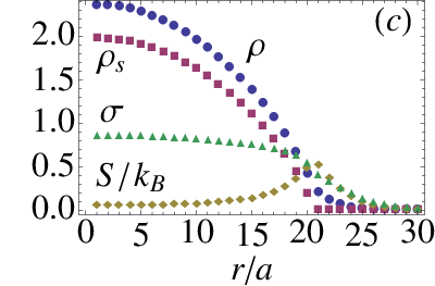
Let us consider the system with the harmonic trapping potential , which usually exists in experiments. Note that is the distance from the center of the trapping potential. In the presence of the trapping potential, the system becomes inhomogenous and has the mixture of SF and N phases. In order to investigate the behavior of the adiabatic heating/cooling in this case, we perform the same calculation as the homogeneous case except inserting the local chemical potential . We take the trapping frequency , the lattice size to be , and the total number density as in the Greiner’s work [16]. Figs. 3 (a) and (b) show qualitativley same results as homogeneous case. The adiabatic cooling occurs in the presence of condensate while the adiabatic heating occurs when there is no condensate. Therefore we can say that the behavior of adiabatic heating/cooling does not change essentially whether there is the trapping potential or not. We note, however, that the effects of the trapping potential is important quantitatively for realizing the strong correlated system as shown in Refs. [12, 19]. In Figs. 3 (c) and (d), we plot the spatial distributions of the occupation number, the condensate density, the entropy, and the number fluctuation along the adiabatic line indicated by two white dots in Figs. 3 (a) and (b). We see the high condensate density in Fig. 3 (c), while the wedding-cake structure is exhibited in Fig. 3 (d). Since we use local density approximation, further detailed studies are needed for the case with the trapping potential.

|

|
|

|
In conclusion, we calculated the three-dimensional Bose-Hubbard model at finite temperatures within the mean-field approximation and investigated the effects of the adiabatic loading of optical lattices to the temperature. The lattice-height dependence of the isentropic curves for given initial temperatures in case of the homogeneous system was computed. We found that the cooling occurs in SF phase while the heating occurs in N phase and the efficiency of the adibatic cooling/heating is higher for higher temperatures. Its behavior is determined by whether the dispersion relation of the system increases or decreases as loading optical lattices. Finally, we showed that the case with the trapping potential is essentially same as the homogeneous one.
Note added. Recently we have become aware of a related paper by Pollet et al. [20]. They studied the adiabatic loading in one-dimensional and two-dimensional optical lattices by quantum monte carlo method. The effect of the trapping potential to the adiabatic loading was investigated with high accuracy in these lower dimensional cases.
Acknowledgements.
S.Y. thanks to S. Miyashita, N. Kawashima, and I. Danshita for fruitful discussions. S.Y. is supported by NAREGI Nanoscience Project from Ministry of Education Culture, Sports, Science, and Technology, Japan. S.K. is supproted by JSPS (Japan Society for the Promotion of Science) Research Fellowship for Young Scientists.References
- [1] D. Jaksch and P. Zoller, Annals of Physics 315, 52 (2005).
- [2] O. Morsch and M. Oberthaler, Rev. Mod. Phys. 78, 179 (2006).
- [3] M.Lewenstein, A.Sanpera, V.Ahufinger, B.Damski, A.S.De, and U.Sen, Adv. Phys. 56, 243 (2007).
- [4] I. Bloch, J. Dalibard, and W. Zwerger, cond-mat/0704.3011 (2007), eprint 0704.3011.
- [5] S. Clark, C. Moura-Alves, and D. Jaksch, New J. Phys. 7, 124 (2005).
- [6] A. Kay, J. Pachos, and C. Adams, Phys. Rev. A 73, 022310 (2006).
- [7] M. Christandl, N. Datta, T. Dorlas, A. Ekert, A. Kay, and A. Labdahl, Phys. Rev. A 71, 032312 (2005).
- [8] D. Jaksch, H.-J. Briegel, J. I. Cirac, C. W. Gardiner, and P. Zoller, Phys. Rev. Lett. 82, 1975 (1999).
- [9] O. Mandel, M. Greiner, A. Widera, T. Rom, and T. Hänsch, Nature 425, 937 (2003).
- [10] P. Blakie and J. Porto, Phys. Rev. A 69, 13603 (2004).
- [11] A. Rey, G. Pupillo, and J. Porto, Phys. Rev. A 73, 23608 (2006).
- [12] T.-L. Ho and Q. Zhou, Phys. Rev. Lett. 99 (2007).
- [13] F. Gerbier, Phys. Rev. Lett. 99 (2007a).
- [14] D. Jaksch, C. Bruder, J. Cirac, C. Gardiner, and P. Zoller, Phys. Rev. Lett. 81, 3108 (1998).
- [15] F. Gerbier, A. Widera, S. Fölling, O. Mandel, T. Gericke, and I. Bloch, Phys. Rev. A 72, 053606 (2005).
- [16] M. Greiner, O. Mandel, T. Esslinger, T. W. Hänsch, and I. Bloch, Nature (London) 45, 39 (2002).
- [17] D. van Oosten, P. van der Straten, and H. Stoof, Phys. Rev. A 63, 053601 (2001).
- [18] X. Lu and Y. Yu, Phys. Rev. A 74, 063615 (2006).
- [19] F. Gerbier, Phys. Rev. Lett. 99, 12045 (2007b).
- [20] L. Pollet, C. Kollath, K. Van Houcke, and M. Troyer, cond-mat/0801.1887 (2008).