Quantum Critical Paraelectrics and the Casimir Effect in Time

In this section we use the self-consistent Gaussian theory to illustrate how the $\chi(T)$ found via FSS in time appears from a more microscopic approach; we also study the crossover behavior between the classical and the quantum critical points. This approach is equivalent to the self-consistent one-loop approximation[36] that is used in the context of metallic magnetism.

The soft-mode treatment has been described extensively elsewhere;[31, 32, 36] here we briefly outline the derivation of the gap equation. The Lagrangian in Euclidean space-time, ${\cal L}_{E}$ in (3), for displacive ferroelectrics is the $\phi^{4}$ model:

which determines the partition function. Notice that in writing (22), we have chosen rescaled units in which the characteristic speed of the soft mode $c_{s}=1$. In a self-consistent Hartree theory, interaction feedback is introduced via its renormalization of quadratic terms; this procedure is equivalent to replacing ${\cal L}_{E}$ by the Gaussian Lagrangian

where

is the Hartree self-energy (see Fig. 4). We note that this mode-mode coupling theory is exact for the “spherical model” generalization of $\phi^{4}$ theory in which the order parameter has $N$ components and $N$ is taken to infinity.

The Green’s function can now be determined from Dyson’s equation, shown diagrammatically in Figure 4, and takes the form

so the action is diagonalized in this basis. The poles of $G(\vec{q},\omega)$ determine the dispersion relation $\omega_{q}$ for the displacive polarization modes

where here we have introduced the gap function

This quantity vanishes at both quantum and classical critical points where there are scale-free (gapless) fluctuations. At the quantum critical point where $T_{c}=0$, $\Delta(r_{c},0)=r_{c}+\Sigma(r_{c},T=0)$, so that we can eliminate $r_{c}=-\Sigma(r_{c},T=0)$, to obtain

where $\Omega_{0}^{2}=(r-r_{c})=g$.

The amplitude of the polarization fluctuations is given by

so the self-consistency (24) condition $\Sigma=3\gamma_{c}\langle P^{2}\rangle$ can now be written

where $\Sigma(r,T)$ is the temperature-dependent self-energy. By converting the discrete Matsubara summation to a contour integral, deformed around the poles $z=\pm\omega(q)$ in the dispersion relation, we can convert this expression to the form

where we denote $n_{B}(\omega)\equiv n_{B}(\omega,\beta)=1/(e^{\beta\omega}-1)$. At the quantum critical point ($r=r_{c}$ and $T=0$), we have $\omega_{q}=q$ and $n(\omega_{q})=0$ so that

and using (28), we can write the gap function as

In the paraelectric phases, we can use the temperature-dependent gap to determine the dielectric susceptibility $\chi$. Writing

we use (25) and (27) to express it as

At the quantum critical point $\Omega_{0}^{2}=0$, so the gap equation (33) becomes

where we have inputted the dispersion relation, (26), for $\omega_{q}$ in (37). We notice that both thermal and quantum fluctuations contribute to this expression.

Even though the mean field gap equation is only formally exact in the spherical mean-field limit, it is sufficient to illustrate the qualitative influence of $T$ on the gap at the QCP. In order to explore the cutoff-dependence of (37), we note that in the ultraviolet limit of interest, the last two terms can be expressed as

where there is complete cancellation when $\Delta=0$ exactly at the QCP. However just slightly away from it, when $\Delta$ is finite, (38) leads to a $q^{d-3}_{max}$ scaling-dependence of the integral in (37); therefore the cutoff is required to ensure that (37) is finite in dimensions $d>3$. However, in dimensions $d<3$, this integral is convergent in the ultraviolet and the upper cutoff in (37) can be entirely removed. Thus, for $d<3$, the only scale in the problem is temperature itself. The integral is also convergent in the infrared provided $d>1$. The spatial dimensions $d=1$ and $d=3$ correspond to spacetime dimensions $D=d+1=2$ and $D=d+1=4$, which are the well-known lower and upper critical dimensions of the $\phi^{4}$ theory. This provides us with a dimensional window $1<d<3$ where inverse temperature acts as a cut-off in time. In this range, the temperature-dependence of the gap

is independent of the strength of the coupling constant $\gamma_{c}$ and the cutoff, a feature that can be illustrated already within mode-coupling theory. Recalling that $\Delta(T)=\frac{\alpha}{L_{\tau}}$ and $\alpha\equiv\alpha_{d}$ (see (13) and Fig.1), we note that confirmation of (39) is consistent with our earlier discussion (see after (12)) that $\xi_{\tau}$ is independent of coupling constant; in this dimensional window, temperature is a boundary effect in (imaginary) time and is the only temporal scale in the problem.

In order to calculate $\alpha_{d}$, we rewrite the gap equation at criticality as

where $\Gamma_{d}q^{d-1}dq$ $(\Gamma_{d}=\frac{2\pi^{d/2}}{\Gamma(d/2)})$ is the d-dimensional volume measure. Rescaling $\Delta=\alpha_{d}T$ and $q=uT$, we obtain

where

For $d<3$, the temperature prefactor on the right-hand side of (41) vanishes $T\rightarrow 0$, so a consistent solution requires $\alpha_{d}$ to satisfy

At a small finite temperature, we can expand around $\alpha=\alpha_{d}+\delta\alpha(T)$, to obtain

Thus in dimensions $d<3$, the dominant low temperature behavior is independent of $\gamma_{c}$, the strength of the mode-mode coupling, which enters into the subleading temperature dependence.

The necessity of separating out the singular part of equation (41) was pointed out to us by Chamati and Tonchev;[37] (41) was incorrectly treated in an earlier version of this paper. Following their approach, we can rewrite (41) as

yielding

provided $(1\leq d\leq 3)$. The first term in this expression is a smooth positive function of $d$ and $\alpha$, whereas the second is a singular negative function of $d$ with poles at $d=1$ and $d=3$. The numerical solution of $F_{d}[\alpha_{d}]=0$ can then be determined and is presented in Fig. 5. We note that this result indicates that $\alpha_{d}$ vanishes in the vicinity of $d\sim 3$ as $\alpha_{d}\sim\sqrt{3-d}$, consistent with previous $\epsilon$ calculations.[23]

In Figure 5 we display the dependence of $\alpha_{d}$ on dimensionality $1<d<3$. The temperature-dependence of the gap in two dimensions is shown in the inset of Fig. 5, where we see that $\lim_{T\rightarrow 0}\alpha_{2}\equiv 0.96$ is the same for all couplings. According to (41) and (42), we write $\alpha_{3}^{2}=\gamma_{c}F_{3}[\alpha]$ and solve for $\alpha_{3}$ in the limit of upper cutoff $u_{max}=q_{max}/T\equiv 2\pi T_{0}/T>>\alpha_{3}$,

where again we do not consider logarithmic corrections to $\alpha_{3}$. In the limit of strong coupling, $\alpha_{3}\sim\big[\ln(\frac{4\pi T_{0}}{T})\big]^{-1/2}$ is $\gamma_{c}$ independent. For weak coupling, the situation relevant here, $\alpha_{3}$ is indeed a function of $\gamma_{c}$ but remains independent of temperature so that $\Delta\sim T$ according to (39); temperature-dependences derived here should therefore be in agreement with those found from a scaling perspective whenever direct comparison is possible.

To provide an explicit illustration of the above calculations, we now use (33), and (36) to numerically determine the temperature-dependent paraelectric susceptibility in the approach to the quantum critical point (QCP) in $d=3$. We obtain $\chi^{-1}(T)=\Delta^{2}\sim T^{2}$ for the approach $r=r_{c}$ in agreement with previous results and discussion. We note that a similar analysis in the vicinity of the classical phase transition leads to the expected Curie susceptibility ($\chi^{-1}(T\rightarrow T_{c}^{+}>>0)\sim T$) since in this (high) temperature regime the Bose function in (37) scales as $\frac{T}{\omega}$. We also remark that if we assume that $\omega\equiv\tilde{\omega}_{0}$ with no q-dependence then we recover the Barrett[38] expression $\chi^{-1}\sim A+B\coth\frac{\hbar\tilde{\omega}_{0}}{k_{B}T}$; because the disperson is constant and q-independent this approach is not applicable near quantum criticality where the gap vanishes and the q-dependence becomes important.

One more point needs to be considered before we proceed with our self-consistent Hartree theory. In the self-consistent Hartree theory (SCHT) of the ferro-electric phase, the polarization field $P_{0}$ acquires a nonzero value. $P_{0}$ enters the Lagrangian ${\cal{L}}_{E}$ in (22) as $P=P_{0}+\delta P$, where $\delta P$ are fluctuations of the polarization field around its mean value, $P_{0}$ ($P_{0}=0$ in the paraelectric phase). The self energy (24) becomes

as indicated diagrammatically in Figure 4. The equilibrium value $P_{0}$ is easily obtained by introducing an electric field into the Lagrangian by replacing ${\cal L}_{E}\to{\cal L}_{E}+E\cdot P$, then seeking the stationary point $\delta S/\delta P_{0}=0$ which gives $\langle rP_{0}+3\gamma_{c}\delta P^{2}P_{0}+\gamma_{c}P_{0}^{3}-E\rangle=0$, or

at zero electric field. According to (27), $\Delta^{2}(r,T)=r+\Sigma(r,T)$, so that the spectral gap in the ferroelectric phase is

In Fig. 6 a) we plot the calculated temperature-dependent spectral gap $\Delta(r,T)$ for three different values of $r$ as indicated in its schematic inset. As expected, for (2) the spectral gap closes exactly at $T=0$ leading to a linear dispersion relation, $\omega=q$ at the QCP. We note that in the quantum paraelectric (QPE), $\Delta$ (or $\chi^{-1}$) is constant. In the quantum ferroelectric (QFE) again $\Delta$ is constant; though there exists a classical paraelectric-ferroelectric transition at $T=T_{c}$ where $\chi^{-1}\sim(T-T_{c})$. The static dielectric susceptibility in the vicinity of the QCP (low T) is presented in the same three $r$ regimes in Fig.6 b) where we see that in the QPE regime $\chi(T\rightarrow 0)$ saturates, at the QCP $\chi(T)\sim T^{-2}$ and diverges as $T\rightarrow 0$. In the QFE, the susceptibility also saturates at low temperatures, though the Curie law is recovered in the vicinity of the classical transition at $T=T_{c}$.

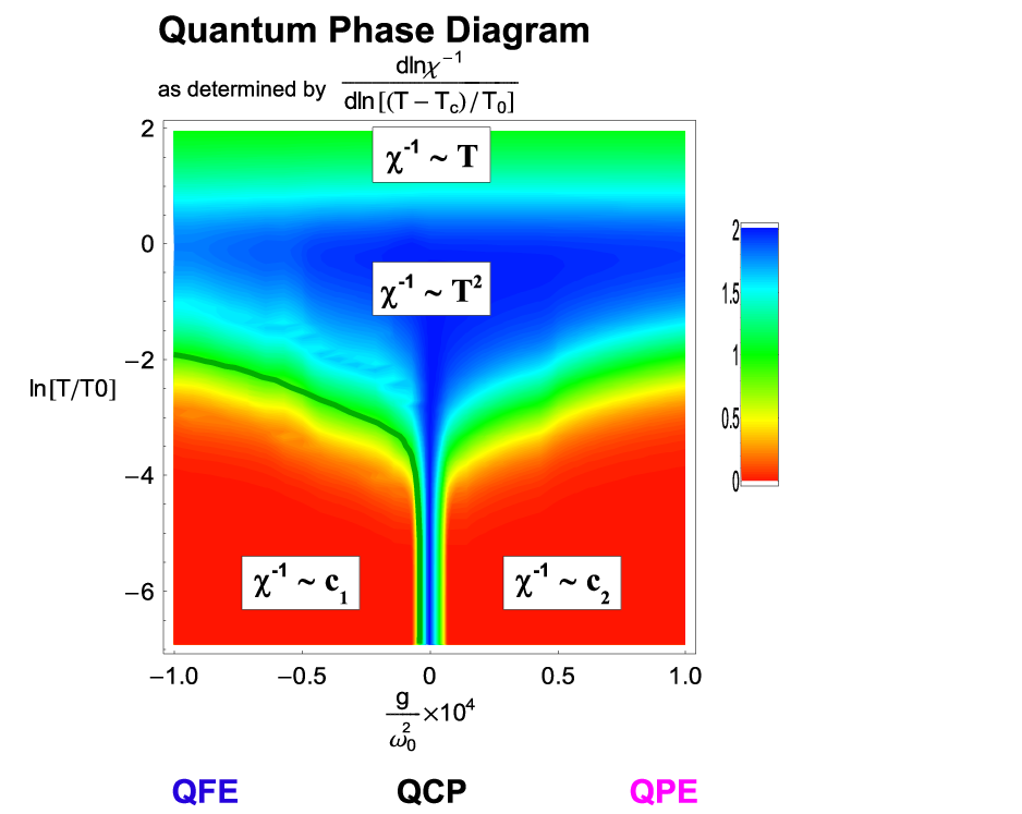
Figure 7 shows the phase diagram that results from the self-consistent Hartree theory. This figure serves to emphasize how the strictly zero temperature QCP gives rise to a quadratic power law dependence of the inverse susceptibility on temperature over a substantial region of the $T-g$ phase diagram.

The crossover temperature, $T_{0}$, between Curie ($\chi^{-1}\sim T$) and Quantum Critical ($\chi^{-1}\sim T^{2}$) behavior in the susceptibility is defined by the expression

where $\omega_{0}=\frac{c_{s}}{a}$ is the characteristic soft mode frequency, $c_{s}$ is the soft-mode velocity and $a$ is the lattice spacing. Here we have assumed a simple bandstructure $\omega(q)=\omega_{0}\sin qa$ such that $c_{s}=\left.\phantom{\int}\frac{d\omega}{dq}\right|_{q=0}=\left.\phantom{\int}(\omega_{0}a)\cos qa\right|_{q=0}$ so so that $\omega_{0}=\frac{c_{s}}{a}$ as stated above. The factor of $2\pi$ in the denominator of (51) results from the observation that the separation of the poles of the Bose and Fermi functions in the complex frequency plane is $\Delta\nu_{n}=2\pi k_{B}T$, which sets the natural conversion factor between temperature and frequency to be $2\pi k_{B}$. $T_{0}$ also corresponds to the temperature when the correlation length is comparable to the lattice constant ($\xi\sim a$); here the correlation length $\xi\equiv\frac{c_{s}}{\Omega_{0}}\sim g^{-1/2}$ (see (17)). Neutron scattering measurements[39] of the dispersion relation indicate that the soft mode velocity in STO is $c_{s}\approx 10^{4}m/s$ and the lattice constant has been measured [40] to be $a_{STO}=3.9\times 10^{-10}m$; therefore $T_{0}\approx 30K$. We note that with $O^{18}$ substitution, the ambient pressure Curie temperature[14] is $T_{c}\sim 25K$. Using the values of $c_{s}$ and $a_{STO}$ from above, we get $\omega_{0}\approx 2.6\times 10^{13}Hz$ in $SrTiO_{3}$. The typical frequency $\Omega_{0}=g^{1/2}$ (spectral gap at zero temperature) at which one observes the change of behavior in the dielectric susceptibility (blue region) is thus from Figure 7, $\Omega_{0}\approx 10^{-2}\>\omega_{0}=2.6\times 10^{11}Hz$. Indeed, Raman scattering on ferroelectric $SrTi^{18}O_{3}$ ($T_{c}=25K$) shows that the zero temperature Raman shift [41] is about $10\>cm^{-1}$ which translates into $\Omega_{0}\approx 3\times 10^{11}Hz$, in good agreement with our calculation.

In a conventional solid, broken translational symmetry leads to three acoustic Goldstone modes. At a ferroelectric QCP, these three modes are supplemented by one or more optical zero modes. This coexistence of acoustic and optic zero modes is a unique property of the ferroelectric QCP, and in this section we examine how their interaction influences observable properties.

The gap of the optical modes in a ferroelectric is sensitive to the dimensions of the unit cell and couples linearly to the strain field. This leads to an inevitable coupling between the critical optical mode and the long-wavelength acoustic phonons that must be considered. To address this issue, we consider the effect of a coupling $\eta$ between the soft polarization and the strain field created by a single long-wavelength acoustic phonon mode. Softening of the polar transverse optic (TO) mode near the QCP enhances the effect of this coupling. Using dimensional analysis we find that the coupling between the TO and LA mode is marginally relevant in the physically important dimension $d=3$, and thus can not be ignored. The main result of the analysis is that the acoustic phonons act to soften and reduce the quartic interaction between the optic phonons. Beyond a certain threshold $\eta>\eta_{c}$, this interaction becomes attractive, leading to the development of a reentrant paraelectric phase at finite temperatures. We note that such a coupling to acoustic phonons has been considered previously,[18] and here we are rederiving and extending prior results in a contemporary framework.

We introduce the coupling of the polarization ($P(\vec{x},\tau)$) and the acoustic phonon ($\phi(\vec{x},\tau)$) fields as a coupling of the polarization to strain $-\eta\nabla\phi P^{2}$; we then write the Lagrangian [18] as

where ${\cal L}_{E}[P]$ is our previous Lagrangian without acoustic coupling given in (22). Here the constant $\eta$ is the coupling strength to the acoustic phonon; the latter’s dynamics are introduced in the bracketed terms of (52). Since we are using units in which the velocity of the soft optical phonon is one, $\tilde{c}=\frac{c_{a}}{c_{s}}$ is the ratio of the acoustic to the soft optical phonon velocities. We will discuss the restoration of dimensional constants in (52) when we make comparison to experiment in Section V. F.

We begin with a dimensional analysis of the couplings to assess their relative importance in the physically important dimension $d=3$. In order to do so, we introduce the renormalization group (RG) flow by rescaling length, time, momentum and frequency

with constant $\Lambda>1$ representing flow away from the infrared (IR) limit of the QCP, that is flow from small to large momentum and frequency. In terms of the rescaled variables $x^{\prime}$ and $\tau^{\prime}$, the action (3) with Lagrangian (52) in $d+1$ dimensions becomes

We emphasize that we write $\Omega_{0}^{2}=r-r_{c}$ as the coefficient of the $P^{2}$ term in the Lagrangian $L_{E}[P]$ (22), entering (52) in (54), since our RG flow starts from the QCP ($r=r_{c}$). Rescaling $P$, $\phi$, $\Omega_{0}^{2}$, $\gamma_{c}$ and $\eta$, so that the action (54) assumes its initial form, we write

which leads to

Now the fields, the mass term and the coupling constants flow to new values leaving the action unperturbed. We remark that the upper cuttoff in the imaginary time dimension is replaced by infinity as the temperature $T\sim\frac{1}{\beta}$ approaches zero.

Analyzing the RG expressions in (57), we find that the $\Omega_{0}^{2}$ term grows as we flow away from the QCP IR limit; therefore it is a relevant perturbation parameter independent of dimension $d$. This is consistent with the fact that $\Omega_{0}^{2}=r-r_{c}=g$ tunes the system away from the QCP. Similarly we find that couplings $\gamma_{c}$ and $\eta$ grow (relevant) in dimension $d<3$, decrease (irrelevant) in dimension $d>3$, and don’t change (marginally relevant) in $d=3$. We see that in this case ($d=3$) the coupling to acoustic phonons ($\eta^{\prime}$) is equally important as the mode-mode coupling ($\gamma_{c}^{\prime}$) and thus has to be included to the Gaussian model.

Let us now briefly summarize what we know about $\gamma_{c}$ before we proceed to the discussion of the acoustic coupling $\eta$. In section IV B we found that the spectral gap $\Delta$ is independent of $\gamma_{c}$ for dimensions $1<d<3$ in the zero temperature limit (see Fig. 5). This is in agreement with the above results, where $\gamma_{c}$ is a relevant perturbative parameter; more precise analysis [1] shows $\gamma_{c}$ flowing to the nontrivial Wilson-Fisher fixed point $\gamma_{c}^{*}$. Here all the system properties become functions of $\gamma_{c}^{*}+\delta\gamma_{c}\approx\gamma_{c}^{*}$, and so are $\gamma_{c}$-independent. On the other hand, in dimensions $d>3$ and $d=3$, $\gamma_{c}$ flows to zero (with logarithmic corrections in the marginal case). In these cases the system properties are functions of $\delta\gamma_{c}$ and thus are $\gamma_{c}$-dependent; we have already seen an example of this behavior in the specific case of the $d=3$ spectral gap.

We are now ready to explore how the system’s low-temperature behavior changes in the presence of acoustic phonons in dimension $d=3$. Let us look first at the LA phonon field $\phi$. Following the procedure of Section IV A, we find the acoustic Green’s function and dispersion relation from (52) to be

We emphasize the $P^{2}$-dependency of the new interaction term, $-\eta\nabla\phi P^{2}$, in the Lagrangian (52). Therefore it contributes to the polarization self-energy as an additional term inside the brackets of (23). This new contribution arises due to nonzero second-order perturbation and is schematically shown in Figure 8, where the solid line represents the soft polarization TO Green’s function (25) and the dashed line represents the LA Green’s function (59). We note that the interaction represented by a dot in the self-energy consists of a contribution each from the coupling $\gamma_{c}$ and $\eta$. Thus we can write the polarization self-energy $\Sigma$ as a sum of these two terms

where $\Sigma_{\gamma_{c}}$ is the Hartree self-energy (30) previously calculated in Section IV A. We remark that the $q^{2}$ term in the integral for $\Sigma_{\eta}$ arises due to form of the interaction ($\nabla\phi$). Converting the Matsubara summation to a contour integral, deformed around the poles $z_{p}=\pm\omega_{p}(q)$ and $z_{a}=\pm\omega_{a}(q)$ in the dispersion relations of the polarization (26) and acoustic phonon (60) modes respectively, we can rewrite $\Sigma_{\eta}$ in the form [18]

Bibliography

- [1] J. Cardy, Scaling and Renormalization In Statistical Physics, (Cambridge University Press, Cambridge, 1999).
- [2] S.L. Sondhi, S.M. Girvan, J.P. Carini and D. Shahar, “Continuous Quantum Phase Transitions,” Rev. Mod. Phys 69, 315 (1997).
- [3] S. Sachdev, Quantum Phase Transitions, (Cambridge University Press, Cambridge 1999).
- [4] M.A. Continentino, Quantum Scaling in Many-Body Systems, (World Scientific, Singapore 2001).
- [5] P. Coleman and A.J. Schofield, “Quantum Criticality,” Nature 433, 226 (2005).
- [6] H.B.G. Casimir, “On the attraction between two perfectly conducting place,” Proc. Kon. Ned. Akad. Wetenschap 51, 793 (1948); H.B.G. Casimir and D. Polder, “The Influence of Retardation on the London-van der Waals Forces,” Phys. Rev. 73, 360 (1948).
- [7] M. Krech, The Casimir Effect in Critical Systems, (World Scientific, Singapore, 1994).
- [8] M. Kardar and R. Golestanian, “The “friction” of vacuum, and other fluctation-induced forces,” Rev. Mod. Phys. 71, 1233 (1999).
- [9] S.K. Lamoreaux, “Demonstration of the Casimir force on the 0.6 to 6 mm range,” Phys. Rev. Let. 78, 5 (1997).
- [10] U. Mohideen and A. Roy, “Precision measurement of the Casimir force from 0.1 to 0.9 m,” Phys. Rev. Lett. 81, 4549 (1998).
- [11] H.B. Chan, V.A. Aksyuk, R.N. Kleiman, D.J. Bishop, F. Capasso, “Quantum Mechanical Actuation of Micromechanical Systems by the Casimir Force,” Science 291, 1941 (2001).
- [12] M. Lisanti, D. Iannuzzi and F. Capasso, “Observation of the skin-depth effect on the Casimir force between metallic surfaces,” PNAS 102, 11989 (2005).
- [13] J.M. Obrecht, R.J. Wild, M. Antezza, L.P. Pitaevskii, S. Stringari and E.A. Cornell, “Measurement of the Temperature-Dependence of the Casimir-Polder Force,” Phys. Rev. Lett. 98, 063201 (2007).
- [14] E.L. Venturini, G.A. Samara, M. Itoh and R. Wang, “Pressure as a probe of the physics of 18O-subsituted ,” Phys. Rev. B 69, 184105 (2004).
- [15] P. Coleman, “Theory Perspective: SCES 05 Vienna,” Physica B 378-380, 1160 (2006).
- [16] S.E. Rowley, L.J. Spalek and S.S. Saxena, “Quantum Criticality in Ferroelectricity”, submitted; S.E. Rowley and S.S. Saxena, private communication.
- [17] A.B. Rechester, “Contribution to the Theory of Second-Order Phase Transitions at Low Temperatures,” Sov. Phys. JETP 33, 423 (1971).
- [18] D.E. Khmelnitskii and V.L. Shneerson, “Low-Temperature Displacement-Type Phase Transition in Crystals,” Sov. Phys.- Solid State 13, 687 (1971); ibid Sov. Phys. JETP 37, 164 (1973).
- [19] R. Roussev and A.J. Millis, “Theory of the quantum paraelectric-ferroelectric transition,” Phys. Rev. B 67, 014105 (2003).
- [20] N. Das and S.G. Mishra, “Fluctuations and Criticality in Quantum Paralectrics,” cond-mat arXiv:0707.2634.
- [21] T. Schneider, H. Beck, and E. Stoll, “Quantum effects in an n-component vector model for structural phase transitions,” Phys. Rev. B 13, 1123 (1976).
- [22] D. Schmeltzer, “Quantum Ferroelectric: A Renrmalization-Group Study,” Phys. Rev. B 27, 459 (1983).
- [23] S. Sachdev, “Theory of Finite-Temperature Crossovers near Quantum Critical Points Close to, or Above, Their Upper-Critical Dimension,”, Phys. Rev. B 55 142 (1997).
- [24] J. Hertz, “Quantum Critical Phenomena” Phys. Rev. B 14, 1165 (1976).
- [25] D. Rytz, U.T. Hochli and H. Bilz, “Dielectric Susceptibility in Quantum Ferroelectrics,” Phys. Rev. B 22, 359 (1980).
- [26] M.E. Fisher and P.G. deGennes, C.R. Acad. Sci. Paris B 287, 207 (1978).
- [27] D.M. Danchev, J.G. Brankov and N.S. Tonchev, Theory of Critical Phenomena in Finite-Size Systems: Scaling and Quantum Effects (World Scientific, Singapore 2000).
- [28] E. Brezin and J. Zinn-Justin, “Finite-Size Effects in Phase Transitions,” Nucl. Phys. B 257 867 (1985).
- [29] J. Rudnick, H. Guo and D. Jasnow, “Finite-Size Scaling and the Renormalization Group,” J. Stat. Phys. 41, 353 (1985).
- [30] H. Chamati D.M. Danchev and N.S. Tonchev, “Casimir amplitudes in a quantum spherical model with long-range interaction,” Eur. Phys. J. B 14, 307 (2000).
- [31] K.A. Muller and H. Burkard, “: An intrinsic quantum paraelectric below 4 K”, Phys. Rev. B 19, 3593 (1979).
- [32] M.E. Lines and A.M. Glass, Principles and Applications of Ferroelectrics and Related Materials, (Oxford University Press, Oxford, 1977).
- [33] R. Wang and M. Itoh, “Suppression of the quantum fluctuation in 18O-enriched strontium titanate,” Phys. Rev. B 64, 174104 (2001).
- [34] M.C. Aronson, R. Osborn, R.A. Robinson, J.W. Lynn, R. Chau, C.L. Seaman, and M.B. Maple, “Non-Fermi-Liquid Scaling of the Magnetic Response in (,),” Phys. Rev. Lett. 75, 725 (1995).
- [35] A. Schroeder, G. Aeppli, R. Coldea, M. Adams, O. Stockert, H. von Lohneyson, E. Bucher, R. Ramazashvili and P. Coleman, “Onset of magnetism in heavy fermion metals”, Nature 407, 351(2000).
- [36] T. Moriya, Spin Fluctuations in Itinerant Electron Magnets (Springer-Verlag, Berlin, 1985).
- [37] H. Chamati and N.S. Tonchev, “Comment on Quantum Critical Paraelectrics and the Casimir Effect in Time,” arXiv:0903.5229.
- [38] J.H. Barrett, “Dielectric Constant in Perovskite Type Crystals,” Phys. Rev. 86, 118 (1952).
- [39] Y. Yamada and G. Shirane, “Neutron Scattering and Nature of the Soft Optical Phonon in ,” J. Phys. Soc. Japan 26, 396 (1969).
- [40] J.H. Haeni, P. Irvin, W. Chang, R. Uecker, P. Reiche, Y.L. Li, S. Choudhury, W. Tian, M.E. Hawley, B. Craigo, A.K. Tagantsev, X.Q. Pan, S.K. Streiffer, L.Q. Chen, S.W. Kirchoefer, J. Levy and D.G. Schlom, “Room-temperature ferroelectricity in strained ,” Nature 430, 758 (2004).
- [41] M. Takesada, M. Itoh and T. Yagi, “Perfect Softening of the Ferroelectric Mode in the Isotope-Exchanged Strontium Titanate of Studied by Light Scattering,” Phys. Rev. Lett. 96, 227602 (2006).
- [42] C. v. K. Schmising, M. Bargheer, M. Kiel, N. Zhavoronkov, M. Woerner, T. Elsaesser, I. Vrejoiu, D. Hesse, and M. Alexe, “Strain Propogation in Nanolayered Perovskites Probed by Ultrafast X-Ray Diffraction,” Phys. Rev. B 73, 212202 (2006).
- [43] R.O. Bell and G. Rupprecht, “Elastic Constants of Strontium Titanate,” Phys. Rev. 129, 90 (1963).
- [44] L. Palova, P. Chandra, and K.M. Rabe, “Modeling the dependence of properties of ferroelectric thin film on thickness,” Phys. Rev. B 76, 014112 (2007).
- [45] N.A. Pertsev, A.G. Zembilgotov, and A.K. Tagantsev, “Effect of Mechanical Boundary Conditions on Phase Diagrams of Epitaxial Ferroelectric Thin Films,” Phys. Rev. Lett. 80, 1988 (1998).
- [46] T. Moriya and J. Kawabata, J. Phys. Soc. Japan 34, 639 (1973); J. Phys. Soc. Japan 35,669 (1973).
- [47] J. A. Hertz, Phys. Rev. B 14, 1165 (1976).
- [48] A. J. Millis, Phys. Rev. B 48, 7183 (1993).
- [49] A.I. Larkin and D.E. Khmel’nitskii, “Phase Transition in Unxiaxial Ferroelectrics,” Sov. Phys. JETP 29, 1123 (1969).
- [50] A. R. Akbarzadeh, L. Bellaiche, K. Leung, J. Iniguez, and D. Vanderbilt, “Atomistic simulations of the incipient ferroelectric ,” Phys. Rev. B 70, 054103 (2004).
- [51] H. Taniguchi and M. Itoh, Phys. Rev. Let. 99 017602 (2007).
- [52] A.J Millis, A.J.Schofield, G.G. Lonzarich and S.A. Grigera, “Metamagnetic Quantum Criticality,” Phys. Rev. Let. 88 217204 (2002).
- [53] P. Gegenwart, Q. Si and F. Steglich, “Quantum Criticality in Heavy-Fermion Metals,” Nature 4, 186 (2008).
- [54] J.W. Kim et al., “Dielectric Constant Increase near the Magnetic-Field Induced Metaelectric Transition in Multiferroic ,” submitted to Nature Physics.
- [55] N. D. Mathur, F. M. Grosche, S. R. Julian, I. R. Walker, D. M. Freye, R. K. W. Haselwimmer, and G. G. Lonzarich, “Magnetically mediated superconductivity in heavy fermion compounds,” Nature 394, 39 (1998).
- [56] B. Laughlin, G. G. Lonzarich, P. Monthoux, and D. Pines, “The quantum criticality conundrum,” Adv. Phys. 50, 361 (2001).
- [57] P. Coleman, C. Pepin, Q. Si, and R. Ramazashvili, “How do Fermi liquids get heavy and die?,” J. Phys.: Condens. Matter 13, 723(R) (2001).
- [58] H. von Löhneysen, A. Rosch, M. Vojta, M., and P. Wolfe, “Fermi-liquid instabilities at magnetic quantum phase transitions,” Rev. Mod. Phys. 79, 1015 (2007).