Optimization of periodic composite structures for sub-wavelength focusing Thanks: This work was partially supported by NSF grant DMS-0537015.
Abstract
Recently, there has been plenty of work in designing and fabricating materials with an effective negative refractive index. Veselago realized that a slab of material with a refractive index of would act as a lens. Pendry suggested that the Veselago lens would act as a superlens, providing a perfect image of an object in contrast to conventional lenses which are only able to focus a point source to an image having a diameter of the order of the wavelength of the incident field.
Recent work has shown that similar focusing effects can be obtained with certain slabs of “conventional” periodic composite materials: photonic crystals. The present work seeks to answer the question of what periodic dielectric composite medium (described by dielectric coefficient with positive real part) gives an optimal image of a point source. An optimization problem is formulated and it is shown that a solution exists provided the medium has small absorption. Solutions are characterized by an adjoint-state gradient condition, and several numerical examples illustrate both the plausibility of this design approach, and the possibility of obtaining smaller image spot sizes than with typical photonic crystals.
keywords
Periodic composite materials, optimization, sub-wavelength focusing.AMS
78-02, 35J20, 49S051 Introduction
Recently, there has been a renewed and avid interest in studying a class of materials known as the left-handed materials (LHMs). These materials have simultaneously negative real parts of dielectric permittivity and magnetic permeability , so that their refractive index is negative. The properties of such meterials were investigated first by Veselago in 1967 [20]. As shown by Veselago, LHMs exhibit some peculiar electromagnetic properties such as negative index of refraction and wave vector, k, and Poynting vector, S, having opposite directions. Veselago realized that a slab of LHM would act as a lens.
Due to the absence of naturally ocurring materials possessing both negative permittivity and negative permeability, Veselago’s predictions did not receive much attention until recently, when a material with both negative permittivity and negative permeability at microwave frequencies was built [19]. Subsequently, the properties of LHMs were analyzed by many authors.
According to Abbe’s diffraction limit, conventional lenses based on positive index materials with curved surfaces are not able to resolve an object’s fine details that are smaller than half of the light wavelength . The limitation occurs because the waves with transverse wave numbers larger than , which carry information about the fine sub- details of the object, decay exponentially in free space. In a negative index material slab, however, the evanescent wave components can grow exponentially and thus compensate for the exponential decay. Therefore, under ideal conditions, all Fourier components from the object can be recovered at the image plane producing a resolution far below the diffraction limit [17].
Milton et al. proved superlensing in the quasistatic regime (where the wavelength is much larger than the object), and discused limitations of superlenses in this regime due to anomalous localized resonance. If the source being imaged responds to an applied field, it must lie outside the resonant regions to be successfully imaged [14].
In the electrostatic limit, the magnetic and electric fields decouple, and the requirement for superlensing of transverse-magnetic waves is reduced to only , where is the permittivity of the host medium interfacing the lens [17]. An example of such near field superlens is a slab of silver in air illuminated at its surface plasmon resonance (where ). Experiments with silver slabs have already shown rapid growth of evanescent waves [10], submicron imaging [13], and imaging beyond the diffraction limit [6]. A major draw-back of such near-field superlenses based on bulk metals is that they can operate only at a single frequency satisfying the lens condition . Shalaev et al. proposed a ”tunable” near-field superlens made of metal-dielectric composites that can operate at any desired visible or near-infrared wavelength with the frequency controlled by the metal filling factor of the composite (here the inhomogeneities are assumed to be much smaller than the wavelength) [1].
It was shown by Efros et al. that a two dimensional photonic crystal made from a non-magnetic dielectric has negative values of both the electric permittivity and the magnetic permeability in some frequency range [4], and the photonic crystal behaves like a real LHM with respect to the propagating modes only. If amplification of evanescents waves occurs, it is due to some other reason; for example, excitation of surface waves by the evanescent waves. Such an amplification may provide an improvement of the image in the near-field region, but it does not affect the image near the far-field focal point [5].
The physical principles that allow negative refraction in photonic crystals arise from the dispersion characteristics of wave propagation in periodic media and are very different from those in LHMs. They also do not require both negative electric permittivity and magnetic permeability [8, 16]. The negative refraction of beams can be described by analyzing the equifrequency surface of the band structures [8, 16, 11]. If the constant-frequency contour is everywhere convex, an incoming plane wave from air will couple to a single mode that propagates into the crystal on the negative side of the boundary, and thus negative refraction in the first band is realized. Luo et al. have shown all-angle negative refraction could be achieved at the lowest band of two-dimensional photonic crystals in the case of [11]. Such all-angle refraction is essential for superlens application. The photonic crystal not only focuses all propagating waves without limitation of finite aperture, but also amplifies at least some evanescent waves, and the unconventional imaging effects are due to the presence of additional near-field light. A perfect lens, made of left-handed materials, focuses all propagating waves and all evanescent waves. The important difference for superlensing with a photonic crystals is that only finite number of evanescent waves is amplified. This is a consequence of Bragg scattering of light to leaky photon modes [12]. The resolution of a photonic-crystal superlens at a single frequency is only limited by its surface period instead of the wavelength [12].
More recently Huang et al. proposed an alternative approach to all-angle negative refraction in two-dimensional photonic crystals. By applying appropriate modifications with surface grating to the flat photonic lens, he is able to focus large and/or far way objects [7].
Inspired by the current research in structures that produce sub-wavelength focusing, we use derivative-based minimization techniques to produce structures that will provide sub-wavelength focus with non-magnetic materials and without the need for negative permittivities. Rather than restricting to designs based on photonic crystal structures, we allow as admissible any periodic composite structure (with fixed period) whose refractive index is bounded above and below by fixed constants. And rather than performing parametric optimization over a small number of variables describing the structure, we use techniques of “topology optimization” in which material distribution is completely arbitrary. We are able to obtain structured that focus a point source that is far away from the lens, and also we can obtain structures that give an image at a chosen distance from the lens. Since structures incorporating gratings are included in our admissible class, such designs will naturally arise through the optimization process if they produce the best possible image.
For simplicity, only the case of “two-dimensional” structures in -parallel polarization is considered. The ideas here should extend to the other polarization case and the full three-dimensional problem, although there are some technical hurdles.
The paper proceeds as follows. In Section 2 we describe the model problem and review a variational formulation of the Helmholtz equation in a periodic geometry. The inclusion of a small amount of energy absorption in the medium allows a uniform upper bound on the norm of the electric field, independent of the particular admissible structure (and thereby preventing resonances). In Section 3 we present the optimization problem and derive the optimality conditions. In Section 4 we depict the numerical experiments and show structures that have produced sub-wavelength focus.
2 Model problem
In this paper we consider time-harmonic electromagnetic wave propagation through nonmagnetic heterogeneous media for which the dielectric coefficient is constant in one direction, i.e. . Assuming that the electric field vector , Maxwell’s equations reduce to the Helmholtz equation
| (1) |
where represents the frequency, and is the dielectric coefficient.
2.1 Periodic structure
Assume that the dielectric coefficient is periodic in the variable
Taking the period to be imposes no loss of generality since any other period can be obtained by rescaling .
Assume that the regions , and are homogeneous, for some fixed constant . In particular, assume for and , that . The slab may contain inhomogeneous material.
Suppose a point source is placed above the slab at the point , which generates the incident field , where is the distance from the source, and is the Hankel function. For , we have the representation
where whenever the argument is positive, and otherwise [15]. It follows that
and
We can rewrite
and
( may fail to converge, but only at the isolated values of for which for some . always converges due to the exponential decay in .)
Above the slab , we separate the solution to (1) into the incident and scattered field: . The scattered field can also be separated by the Fourier transform in ,
Plugging this representation back into (1), and solving for each frequency separately, we find that . The second term on the right corresponds to an incoming wave, which we insist must be zero since we want the scattered field to consist only of outgoing waves. Then . It follows that , and
The linear operator (Dirichlet-to-Neumann map) then defines the relationship between the traces and : . On the boundary , the solution should then satisfy
Define the periodic domain (circle)
Define the first Brillouin zone . To reduce the problem (1) over to a family of problems over , we define for the Floquet transform by
The sum can be considered as a Fourier series in the quasi-momentum variable , with values in . The map is an isomorphism from to the direct product space [9]. Floquet theory assures that the solution can be written
| (2) |
where each function is -periodic in the variable, and satisfies the equation
where . The boundary condition on translates to
where
| (3) |
(here are the Fourier series coefficients of with respect to the -variable). Similar considerations apply at the lower boundary of the slab , where (assuming there is no incoming wave coming from below) we find .
2.2 Existence and uniqueness of solutions
Let , , . Define an admissible class of dielectric coefficients
where , . Given the incident wave generated by the point source at , we must solve the family of problems
| in | (4) | ||||
| on | |||||
for all . Existence and uniqueness of weak solutions, with a uniform bound, may be obtained for .
Lemma 1.
For each with and , problem (4) admits a unique weak solution . Furthermore, there exists a constant depending on , , such that , independent of and .
Proof.
For convenience we drop the subscript on solutions. Define for ,
and
It is straightforward to show that defines a bounded sesquilinear form over , and that is a bounded linear functional on . Weak solutions of (4) solve the variational problem
| (5) |
The sesquilinear form uniquely defines a linear operator such that , and the functional is uniquely identified with an element such that by reflexivity and an abuse of notation. Problem (5) is then equivalently stated
| (6) |
We intend to show that is coercive by establishing a bound for all with .
Integrating by parts in , we see by periodicity that
Let and . Each is a finite set and . We can write
for , . Notice that all satisfy , so the second term on the right hand side of the equation above is real and non-negative. We then have
Assuming , and noticing that the first four terms on the right-hand side are purely real and the last two terms are purely imaginary, we find
For convenience, write , , and . Obviously , and are nonnegative real numbers which depend on (and in the case of ). Although and are essentially independent, must satisfy
| (7) |
With this notation,
Note that in the case , we have . Otherwise, so that , and . Hence, for all , and all satisfying (7),
The bound thus holds for every with and for every with . Given this coercivity bound, direct application of the Lax-Milgram Theorem yields existence of the bounded solution operator for problem (6) such that . Thus .
Given the bound on , a uniform bound follows easily, since is uniformly bounded in . ∎
3 Optimal design
The goal of the optimization is to make a perfect image of the incident field on the opposite side of the slab . A “mirror image” to the incident field converging at the point would look like , where is the conjugate Hankel function. Thus we want the trace
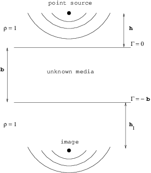
The Bloch representations of and allows us to see that by setting
| (8) |
with defined similarly to , we get .
Problem (4) together with the additional boundary condition (8) is overposed. However, by allowing to vary as a design variable, it may be possible to make (8) hold approximately for each .
3.1 Problem Formulation
Let , where is the weak solution to problem (4).
Consider the minimization
| (9) |
Theorem 2.
The optimization problem has a solution.
Proof.
The proof follows the well-known direct method in the calculus of varations. is weak compact. Consider a minimizing sequence with some subsequence (still denoted by ) converging weak to some . Denote by the solution to the boundary value problem corresponding to . By Lemma (1), the sequence has has a weakly convergent subsequence (still denoted ), in for some . Hence, strongly in . We hold fixed, and we have strongly in . For fixed, as . Here we used the fact that is continuous. Since , as weak . The trace map extends uniquely to a continuous linear operator . Thus, the traces are also convergent: weakly in . This implies weakly in , and, hence, is weak continuous for fixed . But our bound on the solution is independent of , and thus, the minimization problem has at least one solution . ∎
3.2 Adjoint-state derivatives
Let be a ”small” perturbation to the coefficient . We denote the linearization of with respect to by . We have
For fixed ,
and
where solves the linearized problem:
| in | (10) | ||||
| on | |||||
The adjoint of the derivative is the linear operator such that
For all let solve
| in | (11) | ||||
| on | |||||
where . An integration by parts argument shows that
The ”gradient” of the functional is the function for which
where solves (11) with .
Define the normal cones at the minimizer :
and
The gradient is normal to at : . Thus, we have
The continuity of the gradient is sufficient to reduce the above to pointwise optimality conditions. In particular,
for almost every x in .
Similarly,
and the pointwise optimality conditions are:
for almost every x in .
In a similar optimal design problem involving waveguides, one can use the weak continuation property to show [3] that at an optimal , at least one of the four equality bound constraints above on the real and imaginary parts of is attained at almost every point . A similar argument for the present problem is greatly complicated by the form of , involving an integral of a family of PDE solutions, rather than just a single background-adjoint pair. A precise a-priori characterization of optimal solutions is thus difficult.
4 Numerical Results
Approximate solutions of (9) are sought through numerical discretization and optimization. The variational problem (5) was discretized with a first-order finite element method, using piecewise bilinear elements on a uniform, rectangular grid. The design variable was approximated by a piecewise constant function on the same uniform grid. The nonlocal boundary operators defined by (3) were approximated by explicitly calculating the Fourier coefficients of the traces of the finite element basis, then truncating the sum in (3). The resulting finite element scheme can be shown to converge and to conserve energy, provided all the propagating terms are included in the sum [2]. This discretization leads to a large, sparse (except for the boundary terms), non-Hermitian matrix problem, which for simplicity is solved using the direct sparse solver in Matlab.
The integral in (9) was approximated by a discrete sum in . By imposing -axis symmetry in the designs, it suffices to integrate only over positive . In the following examples, we used 20 equally-spaced positive values of to approximate the integral.
Despite the convenience of imposing a positive lower bound on the imaginary part of in Lemma 2.1 for obtaining a uniform upper bound on solutions, we found that the numerical experiments were quite insensitive to small dissipations. Thus in most of the examples below, we set .
After discretizing through finite elements, optimization was accomplished with a straightforward projected gradient descent algorithm as in [3], using the adjoint as derived in Section 3 to calculate the gradient. We performed a large number of numerical experiments with this method, using different initial guesses for the design variable , and varying the frequency , source and focus locations and , and constraints on the real and imaginary parts of .
Generally speaking, we found that the method was able to produce, from almost any initial guess, a structure which produced relatively high field intensity near the desired focus. Some parameter choices and initial guesses resulted in structures with much better focusing properties than others.
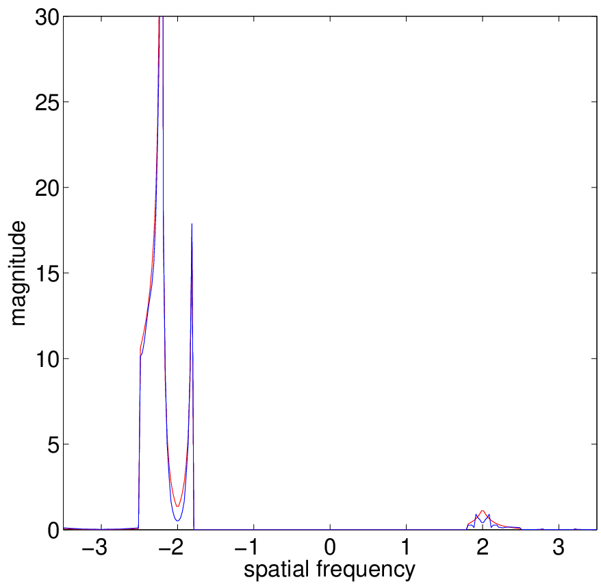
In the first experiment we start with a purely real material and allow the real part of the dielectric coefficient to vary between and . The source is positioned at units from the slab (), and we are looking to obtain a focus units on the opposite side of the slab (). Through numerical optimization we discover the structure shown in Figure 2 which gives a spot size . True subwavelength imaging is only possible if evanescent modes are present at the interface between the structure and the transmission medium. Figure 3 shows the evanescent modes for the generated image versus those of the target, clearly showing that the structure produces evanescent modes which approximate those of the objective.
In the second example we image a source far away from the lens (), and we are looking for the lens that will produce the best image ten units from the lens (). Far away objects are much more difficult to image, but through optimization of the structure, we are able to obtain a spot of size . In the third example we start with a photonic crystal and allow purely real structures varying between and . The source is positioned at units from the slab () and we are looking to obtain a focus four units away on the opposite side of the slab (). The optimized structure is shown in Figure 5, and it gives a focus with spot size , which is much better than the one obtained if we just use photonic crystal as suggested by Luo et al. which produced a focus with spot size [11].
Example four allows both the real and imaginary parts of the dielectric coefficient to vary (, , and , ). The distance between the source and the lens and the distance between the lens and the image are set to four units (, ). The optimized structure gives a focus with a spot size (Figure 6), which is a significant improvement to those obtained by structures described in the research literature so far, although as far as we know, no real materials exist with these dielectric coefficients.
All of the numerical experiments were computationally intensive. Each iteration required the solution of a family of diffraction problems, two for each , and because of the crude optimization method employed, many iterations were typically required. Most of the examples below took on the order of two days to run on a workstation. Since our purpose here was simply to illustrate the feasibility of designing such structures through mathematical optimization, we did not devote much effort to improving the efficiency of the numerical methods. We believe that computation time could be improved by at least an order of magnitude with existing, but more sophisticated, numerical methods.




5 Conclusions
We have demonstrated the feasibility of designing periodic structures with subwavelength focusing properties, via mathematical optimization. The approach is mathematically sound and through numerical discretization yields plausible, if somewhat non-intuitive, solutions.
We point out two weaknesses with the approach presented here, all of which we believe could be improved through further work. First, the performance of the optimized structures tends to be very sensitive to small perturbations in material parameters. This fact combined with the relative complexity of the solutions means that attempting to fabricate these structures is at this point not an attractive idea. Both the sensitivity and the complexity could be addressed through adding appropriate constraints or penalties to the objective. For example, optimization through a level-set approach would necessarily yield structures composed of only two materials, with no intermediate-index areas [18]. This together with total variation penalties may yield “simpler” solutions. Of course such constraints may incur a decrease in the performance of the structure.
Second, the designs created with this approach are not translationally invariant. Specifically, moving the structure laterally relative to the point source may result in decrease of focus. There are a few ways to circumvent this problem. In the simplest case, the distance from the point source to the structure is large so that the wavefront impinging on the structure is nearly planar. Our experiments have shown that in this case focusing is not dependent on the lateral position of the point source (and is much less senstive to vertical translations), although the focus does translate periodically with the structure. One can also optimize for structures whose period is very small compared to the wavelength, although such structures tend to have less focusing power. The ultimate solution to this problem would require building the translation invariance of the focus (not of the medium) into the objective function. Unfortunately this would increase the complexity of the computations beyond the capability of the simplistic approach presented here, but with further work and refinement it should be possible.
References
- [1] W. Cai, D. A. Genov and V.M. Shalaev, Superlens based on metal-dielectric composites, Phys. Rev. B, 72 (2005), 193101
- [2] G. Bao, Finite element approximation of time harmonic waves in periodic structures, SIAM J. Numer. Anal. 32 (1995), 1155–1169.
- [3] D.C. Dobson, Optimal mode coupling in simple planar waveguides, IUTAM Symposium on Topological Design Optimization of Structures, Machines and Materials, M.P. Bendsoe, N. Olhoff, and O. Sigmund, eds., Springer Dordrecht (2006), 311–320.
- [4] A.L. Efros and A.L. Pokrovsky, Dielectric photonic crystals as medium with negative electric permittivity and magnetic permeability, Phys. Rev. B, 68 (2003), 10096
- [5] A.L. Efros, C.Y. Li and J.M. Holt, Far-field Image of Veselago lens, J. Opt. Soc. of A. B, 68 (2006), 60355
- [6] N. Fang, H. Lee, C. Sun, and X. Zhang, Sub-Diffraction-Limited Optical Imaging with a Silver Superlens, Science, 308 (2005), p. 534–537.
- [7] Y.J. Huang, W.T. Lu and S. Sridhar, Alternative approach to all-angle negative refraction in two-dimensional photonic crystals, Phys. Rev. A, 76 (2007), 013824
- [8] C. Luo, S.G. Johnson, J.D. Joannopoulos and J.B. Pendry, Subwave imaging in photonic crystals, Phys. Rev. B, 68 (2003), 10096
- [9] P. Kuchment, Floquet Theory for Partial Differential Equations, Birkhauser, Basel, 1993.
- [10] Z. Liu, N. Fang, T. J. Yen and X. Zhang, Rapid growth of evanescent wave by a silver superlens, Appl. Phys. Lett., 83 (2003), p. 5184–5186
- [11] C. Luo, S.G. Johnson, J.D. Joannopoulos and J.B. Pendry, All-angle negative refraction without negative effective index, Phys. Rev. B, 65 (2002), 201104
- [12] H. Kosaka, T. Kawashima, A. Tomita, M. Notomi, T. Tamamura, T. Sato and S. Kawakami, Superprism phenomena in photonic crystals, Phys. Rev. B, 58(16) (1998), 045115
- [13] D.O.S. Melville, R.J. Blaikie and C.R. Wolf, Submicron imaging with a planar silver lens, Appl. Phys. Lett., 84 (2004), p. 4403–4405
- [14] G.W. Milton, N.P. Nicorovici, R.C. McPhedran and V.A. Podolskiy, A proof of superlensing in the quasistatic regime, and limitations of superlenses in this regime due to anomalous localized resonance, Proc. R. Soc. A, 461 (2005), p. 3999–4034.
- [15] P. Morse and H. Feshbach, Methods of Theoretical Physics, McGraw Hill, New York, 1953, p. 823.
- [16] M. Notomi, Theory of light propagation in strongly modulated photonic crystals: Refractionlike behavior in the vicinity of the photonic band gap, Phys. Rev. B, 62(16) (1996), 10696
- [17] J.B. Pendry, Negative refraction makes a perfect lens, Phys. Rev. Lett., 85 (2000), p. 3966–3969
- [18] F. Santosa, A level-set approach for inverse problems involving obstacles, Control, Optimization, and Calculus of Variations 1 (1996).
- [19] R.A. Shelby, D.R. Smith, and S. Schultz, Experimental Verification of a Negative Index of Refraction, Science, 292 (2001), p. 77–79.
- [20] V.G. Veselago, The electrodynamics of substances with simultaneously negative value of and , Uspehi Fizicheskikh Nauk., 92 (1967), p. 517–526. [English transl. in Soviet Physics Uspekhi, 10 (1968), p. 509–514.