Mass effects and four-particle amplitudes at the two-loop level in QCD
Abstract:
I review the recent progress in the evaluation of two-loop massive QCD amplitudes necessary for the description of hadronic scattering processes at the LHC. I put a special emphasis on the case of top-quark final states.
October 1-5, 2007
Florence, Italy
1 Introduction
There are just a few processes, yet to be observed at the LHC, which require a true NNLO analysis matching a foreseen experimental precision at the percent level. One of the most notable such processes is top-quark pair production. Since the current NLO prediction has a scale dependence of the order of 13% [1] and soft-gluon resummations [2, 3, 4] are not reliable, the case for conducting a complete analysis at the next order of perturbation theory is well grounded.
Here, I review results, which have been obtained thanks to recent advances in the understanding of the application of the factorization theorem to collinear limits [5] on the one hand, and to progress in the evaluation of massive amplitudes started in [6, 7] on the other. By combining the methods, the leading asymptotics in the high-energy regime of the virtual amplitudes have been derived in [8, 9]. From then on, the direct evaluation approach has also provided power corrections in the mass and fully numerical solutions that cover the whole kinematically interesting range [10].
2 Leading asymptotics
Based on experience, it is relatively clear that the logarithmic terms of the expansion of any observable in any limit should be much easier to obtain than the full result. How to actually derive them in the case of collinearly singular limits has been first worked out for Bhabha scattering [11]. Later on, it turned out that even the constant should be within reach thanks to the use of factorization properties of amplitudes [12]. For QCD, the full procedure has been presented in [5] (for application in the context of Bhabha scattering see [13]). Until now, the only part that poses problems is the one due to contributions of closed heavy particle loops, since they actually generate soft singularities, which are process dependent in the sense, that they involve a non-trivial color flow between different external legs.
Let us expand the top-quark pair production amplitude in the strong coupling constant as follows
| (1) |
If the production process involves quark pair annihilation, one can perform the following color decomposition of color averaged amplitudes
| (2) | |||||
where is the number of colors, the number of heavy quarks and the number of light quarks. As noted above, all terms which are free of heavy-quark loops, i.e. can be obtained from factorization. Although the term involves heavy quark loops, it is simple enough to be inferred analogously to the remaining ones. In principle, to complete the expression, one would only have to compute and . These contributions are particularly easy to evaluate with the help of methods based on Mellin-Barnes representations [14, 15, 17, 16]. The results for all the coefficients have been presented in [8], where the authors also checked the factorization formalism by computing directly the , and coefficients finding, as expected, perfect agreement. The interested reader is encouraged to consult [8] for a detailed description of the techniques used. Here, I should only stress that the evaluation of the subleading color coefficients is substantially more complicated due to the occurrence of non-planar graphs. In the mean time, however, all the coefficients have been obtained by the present author, confirming the published results.
Similarly to the quark annihilation channel, the averaged amplitude in the gluon fusion channel can be decomposed as follows
| (3) | |||||
The results for all the coefficients have been given in [9]. The direct computation covered , whereas the factorization formalism provided , , , , , , , , , , , , . Note that this time it was impossible not to compute non-planar graphs, since part of the heavy quark loop contributions involved them. The direct computation of the coefficients covered by factorization only is still under way, since it is necessary for the evaluation of the full amplitude.
3 Power corrections
Due to parton fluxes, a substantial part of top quark pairs will be produced relatively close to threshold. It should, therefore, be clear that the high-energy asymptotics described in the previous section is insufficient for practical purposes. An exact evaluation of the amplitude seems to be out of reach at present, but one can expand in the mass. Introducing
| (4) |
where and are the momenta of the incoming partons and is the momentum of the outgoing top-quark, and
| (5) |
With and , which corresponds to 90 degree scattering, the expansion of the bare leading color term is
![[Uncaptioned image]](0803.1414v1/series.png) |
(6) |
This result in itself looks promising, because we observe asymptotic convergence of the series even at threshold. Unfortunately, the subleading color coefficients cannot behave so nicely, as they contain Coulomb singularities. Moreover, the series suffers from convergence problems for small and large angles as depicted in Fig. 1.


Further discussion and details can be found in [10].
4 Numerical solutions
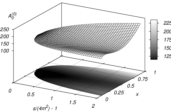
As the discussion of the previous section shows, it is impossible to proceed further without evaluating the amplitude in the threshold region. It turns out that this can be done efficiently with the method of differential equations [18, 19, 20] (for previous applications to physical processes see [21, 22]). The results for the bare leading color coefficient are shown in Fig. 2. For the details the reader is deferred again to [10].
5 Conclusions
Although there is still some work to be done before obtaining a true NNLO prediction for the total cross section for the top-quark pair production cross section, we are at the stage where the virtual amplitudes are almost known (notice that the one-loop squared contributions are known since [23, 24]). The real-virtual corrections are mostly known thanks to the +jet calculation [25] and the necessary phase space integrations of the real radiation corrections can be done with the help of sector decomposition [26, 27], which would then complete the program. Let me also note that similar progress has been obtained in the case of gauge-boson pair production [28] (here, the gauge boson pair production with an additional jet has been studied very recently in [29, 30]).
References
- [1] P. Nason, S. Dawson and R.K. Ellis, Nucl. Phys. B303 (1988) 607.
- [2] E. Laenen, J. Smith and W. L. van Neerven, Nucl. Phys. B 369 (1992) 543.
- [3] R. Bonciani, S. Catani, M. L. Mangano and P. Nason, Nucl. Phys. B 529 (1998) 424.
- [4] N. Kidonakis and R. Vogt, Phys. Rev. D 68 (2003) 114014.
- [5] A. Mitov and S. Moch, JHEP 05 (2007) 001.
- [6] M. Czakon, J. Gluza and T. Riemann, Phys. Rev. D71 (2005) 073009.
- [7] M. Czakon, J. Gluza and T. Riemann, Nucl. Phys. B751 (2006) 1.
- [8] M. Czakon, A. Mitov and S. Moch, Phys. Lett. B651 (2007) 147.
- [9] M. Czakon, A. Mitov, and S. Moch, arXiv:0707.4139 [hep-ph].
- [10] M. Czakon, arXiv:0803.1400 [hep-ph].
- [11] E. W. N. Glover, J. B. Tausk and J. J. Van der Bij, Phys. Lett. B 516 (2001) 33.
- [12] A. A. Penin, Phys. Rev. Lett. 95 (2005) 010408.
- [13] T. Becher and K. Melnikov, JHEP 0706 (2007) 084.
- [14] V.A. Smirnov, Phys. Lett. B460 (1999) 397.
- [15] J.B. Tausk, Phys. Lett. B469 (1999) 225.
- [16] M. Czakon, Comput. Phys. Commun. 175 (2006) 559.
- [17] C. Anastasiou and A. Daleo, JHEP 0610 (2006) 031.
- [18] A. V. Kotikov, Phys. Lett. B 254 (1991) 158.
- [19] E. Remiddi, Nuovo Cim. A 110 (1997) 1435.
- [20] M. Caffo, H. Czyz and E. Remiddi, Nucl. Phys. B 634 (2002) 309.
- [21] R. Boughezal, M. Czakon and T. Schutzmeier, JHEP 0709 (2007) 072.
- [22] M. Czakon and T. Schutzmeier, arXiv:0712.2762 [hep-ph].
- [23] J.G. Korner, Z. Merebashvili and M. Rogal, Phys. Rev. D73 (2006) 034030.
- [24] J.G. Korner, Z. Merebashvili and M. Rogal, arXiv:0802.0106 [hep-ph].
- [25] S. Dittmaier, P. Uwer and S. Weinzierl, Phys. Rev. Lett. 98 (2007) 262002.
- [26] T. Binoth and G. Heinrich, Nucl. Phys. B 585 (2000) 741.
- [27] T. Binoth and G. Heinrich, Nucl. Phys. B 693 (2004) 134.
- [28] G. Chachamis, M. Czakon and D. Eiras, arXiv:0802.4028 [hep-ph].
- [29] S. Dittmaier, S. Kallweit and P. Uwer, Phys. Rev. Lett. 100 (2008) 062003.
- [30] J. M. Campbell, R. Keith Ellis and G. Zanderighi, JHEP 0712 (2007) 056.