Recently, higher dimensional black holes have attracted much interest [1]. In addition to Myers-Perry black holes [2], which have been found as the higher dimensional generalization of Kerr black holes, there are many exotic black holes in higher dimensions [3, 4, 5, 6, 7, 8, 9, 10, 11]. It is quite important to study the stability of these black holes.

The stability of higher dimensional Schwarzschild black holes has been shown [12, 13, 14]. For Myers-Perry black holes, the stability analysis is more difficult because of the difficulty of separation of gravitational perturbation equation.¹¹ 1 The separability of geodesic Hamilton-Jacobi equations, Klein-Gordon equations and Dirac equations in the Myers-Perry spacetime have been shown in Refs. [15, 16, 17, 18, 19, 20, 21, 22, 23, 24, 25, 26, 27, 28, 29, 30, 31]. Nevertheless, there have been several works on the stability analysis. In the case of Myers-Perry black holes with equal angular momenta in odd dimensions higher than five, it was shown that the special modes can be reduced to single ordinary differential equations. For these specific modes, the stability has been shown [32]. In the case of five-dimensional Myers-Perry black holes with equal angular momenta, we have developed a method of analyzing the stability by focusing on the spacetime symmetry $U(2)$ [33]. This method has been proved to be useful for the stability analysis of other $U(2)$ symmetric black holes [34, 35]. The purpose of this work is to study the stability of five-dimensional Myers-Perry black holes with equal angular momenta by making use of our method. We extend the previous stability analysis of Myers-Perry black holes with equal angular momenta [36].

The organization of this paper is as follows. In §2, we introduce Myers-Perry black holes with equal angular momenta and discuss the spacetime symmetry. In §3, we explain how to find master variables with which one can deduce single ordinary equations. In §4, the master equation for most symmetric mode is derived. The stability for this case is analytically shown. In §5, the master equations for other modes are derived and the stability of Myers-Perry black holes for these modes is numerically shown. The final section is devoted to conclusions. In Appendices A and B, detailed calculations for deriving master equations are shown.

In this section, we introduce five-dimensional Myers-Perry black holes with equal angular momenta and clarify the symmetry of the spacetime.

The metric is given by²² 2 In our previous work [33], we used a different coordinate. To put the metric into this form, we need the coordinate transformation $r^{2}+a^{2}\rightarrow r^{2}$ and a change of the parameter $m\rightarrow 2\mu$.

where

and parameters $\mu$ and $a$ are defined for $\mu\geq 0$ and $a^{2}\leq\mu/2$. Here, we define the invariant forms $\sigma^{a}\,(a=1,2,3)$ of $SU(2)$ satisfying the relation $d\sigma^{a}=1/2\epsilon^{abc}\sigma^{b}\wedge\sigma^{c}$ as

and made a combination

The coordinate ranges are $0\leq\theta<\pi$, $0\leq\phi<2\pi$, and $0\leq\psi<4\pi$. The dual vectors of $\sigma^{a}$ are given by

and, by definition, they satisfy the relation $\sigma^{a}_{i}{e}^{i}_{b}=\delta^{a}_{b}$.

The horizon $r=r_{+}$ is found by solving $G(r_{+})=0$, namely,

The angular velocity of the horizon is given by

In term of $r_{+}$ and $\Omega_{H}$, the two parameters $(a,\mu)$ in the metric (1) can be rewritten as

We see the the upper bound of the angular velocity,

Apparently, the metric (1) has the $SU(2)$ symmetry characterized by Killing vectors $\xi_{\alpha}\ ,(\alpha=x,y,z)$:

The symmetry can be explicitly shown by using the relation $\mathcal{L}_{\xi_{\alpha}}\sigma^{a}=0$, where $\mathcal{L}_{\xi_{\alpha}}$ is a Lie derivative along the curve generated by the vector field $\xi_{\alpha}$. From the metric (1), we can also read off the additional $U(1)$ symmetry, which keeps part of the metric, $\sigma^{+}\sigma^{-}$, invariant. Thus, the symmetry of five-dimensional degenerate Myers-Perry black hole becomes $SU(2)\times U(1)\simeq U(2)$.³³ 3 The spacetime (1) also has a time translation symmetry generated by $\partial/\partial t$. Because of this symmetry, we can separate the time dependence of fields as $\propto e^{-i\omega t}$. However, this is obvious and we will not pay much attention to this symmetry hereafter. The Killing vectors ${e}_{3},\xi_{x},\xi_{y}$ and $\xi_{z}$ constitute the symmetry, i.e., ${e}_{3}$ is a generator of $U(1)$ and $\xi_{\alpha}\,(\alpha=x,y,z)$ are generators of $SU(2)$.

Let us define the two kinds of angular momentum operators

where $\alpha,\beta,\cdots=x,y,z$ and $a,b,\cdots=1,2,3$. They satisfy the commutation relations

where $\epsilon_{\alpha\beta\gamma}$ and $\epsilon_{abc}$ are antisymmetric tensors that satisfy $\epsilon_{123}=\epsilon_{xyz}=1$. Note that $L^{2}\equiv L_{\alpha}^{2}=W_{a}^{2}$. The symmetry group, $U(2)\simeq SU(2)\times U(1)$, is generated by $L_{\alpha}$ and $W_{3}$. Here, we should note the fact that

Let us construct the representation of $U(2)$. The eigenfunctions of $L^{2}$ are degenerate, but can be completely specified by eigenvalues of other operators $L_{z}$ and $W_{3}$. They are called Wigner functions and are defined as

where $J=0,1/2,1,3/2\cdots$ and $M,K=-J,-J+1,\cdots,J$. From Eqs. (14), we see that $D^{J}_{KM}$ forms the irreducible representation of $U(2)\simeq SU(2)\times U(1)$. The Wigner functions are functions of $(\theta,\phi,\psi)$ and satisfy the orthonormal relation:

The following relations are useful for later calculations

where we have defined $W_{\pm}=W_{1}\pm iW_{2}$ and $\epsilon_{K}=\sqrt{(J+K)(J-K+1)}$. From this relation, we obtain the differential rule of Wigner functions as

where we have defined $\partial_{\pm}\equiv e_{\pm}^{i}\partial_{i}$ and $\partial_{3}\equiv e_{3}^{i}\partial_{i}$.

For the stability analysis of the Myers-Perry black hole (1), it is necessary to find master equations for metric perturbations. Because Myers-Perry spacetime (1) has the $U(2)$ symmetry, a group theoretical method with a twist can be used  [33, 37]. In this section, we explain a way to find master variables. Once the master variables are found, we can deduce the master equations from the gravitational perturbation equations

where $\nabla_{\mu}$ denotes the covariant derivative with respect to $g_{\mu\nu}$, and we have defined $g_{\mu\nu}\rightarrow g_{\mu\nu}+h_{\mu\nu}$ and $h=g^{\mu\nu}h_{\mu\nu}$.

Now, we consider the mode expansion of $h_{\mu\nu}$. The metric perturbation can be classified into three parts, $h_{AB},h_{Ai}$ and $h_{ij}$ where $A,B=t,r$ and $i,j=\theta,\phi,\psi$. They behave as a scalar, vector and tensor for coordinate transformations of $\theta,\phi$ and $\psi$, respectively. The scalar $h_{AB}$ can be expanded by Wigner functions immediately as

Here, we have omitted the indices $J$ and $M$ because the differential rule of Wigner function (17) cannot shift $J$ and $M$ and therefore the modes with different eigenvalues $J$ and $M$ are trivially decoupled in the perturbation equations.

To expand the vector part $h_{Ai}$, we need an elaborate method. First, we change the basis $\{\partial_{i}\}$ to $\{{e}^{a}\}$, that is, $h_{Ai}=h_{Aa}\sigma^{a}_{i}$ where $a=\pm,3$. Then, because $h_{Aa}$ is scalar, we can expand it, using Wigner functions as

In the expansion of $h_{A+}$, $h_{A-}$ and $h_{A3}$, we shift the index $K$ of Wigner functions, for example, $h_{A+}$ is expanded as $\sum_{K}h_{A+}^{K}D_{K-1}$. The reason is as follows. The invariant forms $\sigma^{\pm}$ and $\sigma^{3}$ have the $U(1)$ charge $\pm 1$ and $0$, respectively (see Eq. (13)), while Wigner function $D_{K}$ has the $U(1)$ charge $K$ (see Eq. (14)). Therefore, by shifting the index $K$, we can assign the same $U(1)$ charge $K$ to $\sigma^{+}_{i}D_{K-1}$, $\sigma^{-}_{i}D_{K+1}$ and $\sigma^{3}_{i}D_{K}$ in Eq. (20).

The expansion of tensor part $h_{ij}$ can be carried out in a similar way as

To assign the same $U(1)$ charge $K$ to each term, we shift the index $K$ of Wigner functions.

Substituting Eqs. (19), (20) and (21) into the perturbation equations (18), we obtain the equations for each mode labelled by $J$, $M$ and $K$. Because of $U(2)$ symmetry, different eigenmodes cannot appear in the same equation.

It is interesting that we can find master variables from the above information. First, we should note that coefficients of the expansion have different indices $K$ and, therefore, coefficients of components $h_{AB}^{K}$, $h_{Aa}^{K}$ and $h_{ab}^{K}$ are restricted as follows:

For example, for the $J=0$ mode, we can classify the metric perturbation as follows:

In the above table, variables in each row can couple with each other. Apparently, $h_{\pm\pm}$ are decoupled, hence, it is straightforward to obtain the master equation for these variables. Other variables, $(h_{A+},h_{+3})$, $(h_{AB},h_{A3},h_{+-},h_{33})$ and $(h_{A-},h_{-3})$, are coupled in each set. However, after fixing the gauge degrees of freedom, we have the master equation for each set. In total, there are five master equations, which matches the physical degrees of freedom of the tensor perturbations at this level. We can continue this analysis. For $J=1/2$ modes, we have the following table:

From the above analysis, we see that $(J,M,K=\pm(J+2))$ modes are always decoupled. Each mode can be reduced to the single master equation. Thus, we have shown that we obtain an infinite number of master equations for the metric perturbations, although they are not everything.

Because of the relations $h_{--}^{\ast}=h_{++}$, $h_{A-}^{\ast}=h_{A+}$ and $h_{-3}^{\ast}=h_{+3}$, we see that $(J,M,-K)$ modes are complex conjugate of $(J,M,K)$ modes. Therefore, we will assume $K\geq 0$ in the following sections.

In the previous section, we showed how to find master variables. In this section, we will derive the master equation for the $J=M=K=0$ mode and show the stability for this mode. The stability for this mode has previously been shown in Ref. [36]. However, we will show the stability again using our formalism.

For the $(J=0,M=0,K=0)$ mode, we must consider metric components $h_{tt},h_{tr},h_{rr},h_{t3},h_{r3},h_{+-}$ and $h_{33}$. We set $h_{\mu\nu}$ as

where ${\rm Re}$ represents the real part of a complex quantity. With the gauge parameters

the gauge transformations for those components are given by

where ${}^{\prime}\equiv\partial_{r}$ and $\delta$ represents the gauge transformation defined by $\delta h_{\mu\nu}=\nabla_{\mu}\xi_{\nu}+\nabla_{\nu}\xi_{\mu}$. The following gauge conditions fix the gauge degrees of freedom completely:

Substituting Eqs. (22) and (25) into Eq. (18), we obtain a set of ordinary differential equations. These equations can be found in Appendix A. Eliminating $h_{tr},h_{rr}$ and $h_{r3}$ from these equations, we obtain the Schrödinger-type master equation,

where we define the new variable

and the tortoise coordinate

The potential $V_{0}$ is given by

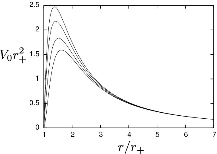
To prove the stability, we must show the positivity of $V_{0}$. The typical profiles of $V_{0}$ shown in Fig. 1 indicate that the potential is always positive. In fact, the positivity can be proved from the expression (29). To see the positivity of $V_{0}(r)$, we focus on $r^{6}$, $r^{4}$ and $r^{0}$ terms in the big bracket in Eq. (29). After dividing them by $16\mu^{4}a^{6}$, we collect them as

If $f(r)$ is positive, $V_{0}(r)$ is also positive. From Eq. (6), we see $\mu\leq r_{+}^{2}$ and $a^{2}\leq r_{+}^{2}/2$. Therefore,

This proves the stability for the $J=M=K=0$ mode.

References

• [1] R. Emparan and H. S. Reall, arXiv:0801.3471 [hep-th].
• [2] R. C. Myers and M. J. Perry, Annals Phys. 172, 304 (1986).
• [3] G. T. Horowitz and A. Strominger, Nucl. Phys. B 360, 197 (1991).
• [4] R. Emparan and H. S. Reall, Phys. Rev. Lett. 88, 101101 (2002) [arXiv:hep-th/0110260].
• [5] A. A. Pomeransky and R. A. Sen’kov, arXiv:hep-th/0612005.
• [6] H. Elvang and P. Figueras, JHEP 0705, 050 (2007) [arXiv:hep-th/0701035].
• [7] H. Iguchi and T. Mishima, Phys. Rev. D 75, 064018 (2007) [arXiv:hep-th/0701043].
• [8] J. Evslin and C. Krishnan, arXiv:0706.1231 [hep-th].
• [9] Y. Morisawa, S. Tomizawa and Y. Yasui, arXiv:0710.4600 [hep-th].
• [10] K. Izumi, arXiv:0712.0902 [hep-th].
• [11] H. Elvang and M. J. Rodriguez, arXiv:0712.2425 [hep-th].
• [12] H. Kodama and A. Ishibashi, Prog. Theor. Phys. 110, 701 (2003) [arXiv:hep-th/0305147].
• [13] A. Ishibashi and H. Kodama, Prog. Theor. Phys. 110, 901 (2003) [arXiv:hep-th/0305185].
• [14] R. A. Konoplya and A. Zhidenko, Nucl. Phys. B 777, 182 (2007) [arXiv:hep-th/0703231].
• [15] G. W. Gibbons and C. A. R. Herdeiro, Class. Quant. Grav. 16, 3619 (1999) [arXiv:hep-th/9906098].
• [16] V. P. Frolov and D. Stojkovic, Phys. Rev. D 67, 084004 (2003) [arXiv:gr-qc/0211055].
• [17] V. P. Frolov and D. Stojkovic, Phys. Rev. D 68, 064011 (2003) [arXiv:gr-qc/0301016].
• [18] H. K. Kunduri and J. Lucietti, Phys. Rev. D 71, 104021 (2005) [arXiv:hep-th/0502124].
• [19] H. K. Kunduri and J. Lucietti, Nucl. Phys. B 724, 343 (2005) [arXiv:hep-th/0504158].
• [20] V. P. Frolov and D. Kubiznak, arXiv:gr-qc/0605058.
• [21] D. Kubiznak and V. P. Frolov, Class. Quant. Grav. 24, F1 (2007) [arXiv:gr-qc/0610144].
• [22] D. N. Page, D. Kubiznak, M. Vasudevan and P. Krtous, Phys. Rev. Lett. 98, 061102 (2007) [arXiv:hep-th/0611083].
• [23] V. P. Frolov, P. Krtous and D. Kubiznak, JHEP 0702, 005 (2007) [arXiv:hep-th/0611245].
• [24] P. Krtous, D. Kubiznak, D. N. Page and V. P. Frolov, JHEP 0702, 004 (2007) [arXiv:hep-th/0612029].
• [25] P. Krtous, D. Kubiznak, D. N. Page and M. Vasudevan, Phys. Rev. D 76, 084034 (2007) [arXiv:0707.0001 [hep-th]].
• [26] T. Houri, T. Oota and Y. Yasui, J. Phys. A 41, 025204 (2008) [arXiv:0707.4039 [hep-th]].
• [27] T. Houri, T. Oota and Y. Yasui, Phys. Lett. B 656, 214 (2007) [arXiv:0708.1368 [hep-th]].
• [28] T. Oota and Y. Yasui, Phys. Lett. B 659, 688 (2008) [arXiv:0711.0078 [hep-th]].
• [29] A. Sergyeyev and P. Krtous, Phys. Rev. D 77, 044033 (2008) [arXiv:0711.4623 [hep-th]].
• [30] V. P. Frolov, arXiv:0712.4157 [gr-qc].
• [31] V. P. Frolov and D. Kubiznak, arXiv:0802.0322 [hep-th].
• [32] H. K. Kunduri, J. Lucietti and H. S. Reall, Phys. Rev. D 74, 084021 (2006) [arXiv:hep-th/0606076].
• [33] K. Murata and J. Soda, Class. Quant. Grav. 25, 035006 (2008) [arXiv:0710.0221 [hep-th]].
• [34] M. Kimura, K. Murata, H. Ishihara and J. Soda, arXiv:0712.4202 [hep-th].
• [35] H. Ishihara, M. Kimura, R. A. Konoplya, K. Murata, J. Soda and A. Zhidenko, arXiv:0802.0655 [hep-th].
• [36] P. Bizon, T. Chmaj, G. W. Gibbons and C. N. Pope, Class. Quant. Grav. 24, 4751 (2007) [arXiv:hep-th/0701190].
• [37] B. L. Hu, J. Math. Phys. 15, 1748 (1974).
• [38] W. H. Press, S. A. Teukolsky, Astrophys. J. 185, 649 (1973)
• [39] R. Gregory and R. Laflamme, Phys. Rev. Lett. 70 (1993) 2837 [arXiv:hep-th/9301052].
• [40] R. Emparan and R. C. Myers, JHEP 0309, 025 (2003) [arXiv:hep-th/0308056].
• [41] G. W. Gibbons, H. Lu, D. N. Page and C. N. Pope, Phys. Rev. Lett. 93, 171102 (2004) [arXiv:hep-th/0409155].
• [42] G. W. Gibbons, H. Lu, D. N. Page and C. N. Pope, J. Geom. Phys. 53, 49 (2005) [arXiv:hep-th/0404008].
• [43] S. W. Hawking, C. J. Hunter and M. Taylor, Phys. Rev. D 59, 064005 (1999) [arXiv:hep-th/9811056].
• [44] S. W. Hawking and H. S. Reall, Phys. Rev. D 61, 024014 (2000) [arXiv:hep-th/9908109].
• [45] V. Cardoso and O. J. C. Dias, Phys. Rev. D 70, 084011 (2004) [arXiv:hep-th/0405006].
• [46] V. Cardoso, O. J. C. Dias and S. Yoshida, Phys. Rev. D 74, 044008 (2006) [arXiv:hep-th/0607162].
• [47] H. Kodama, arXiv:0711.4184 [hep-th].
• [48] B. M. N. Carter and I. P. Neupane, Phys. Rev. D 72, 043534 (2005) [arXiv:gr-qc/0506103].
• [49] P. A. M. Dirac, Lectures on Quantum Mechanics, Dover Pubns, 2001