Collisional statistics of the hard-sphere gas

We consider a hard sphere gas in $d$ dimensions composed of $N$ particles of equal mass $m$ and equal diameter $\sigma$. The gas is thermalized at some temperature $T_{0}$ in a homogeneous state of (constant) density $\rho$, so that the one point distribution function of the system is a Gaussian:

If one decides to follow the evolution of one particle among the $N$, then the velocity probability distribution function (pdf) of that particle will evolve according to the homogeneous linear Boltzmann equation:

where $\ell=(\sigma^{d-1}\rho\chi)^{-1}$ is a length proportional to the mean free path denoted $l$ below, and ${\bf v}_{12}={\bf v}_{1}-{\bf v}_{2}$ . The factor $\chi$ is the pair correlation function at contact and is the so called Enskog correction factor [5]. In the dilute limit where the molecular chaos assumption is justified, it tends to unity. Moreover, the primed integral means that the integration has to be performed in the domain for which ${\bf v}_{12}\cdot\hat{\boldsymbol{\sigma}}>0$. Finally, we are employing the short-hand notation $f^{**}_{i}\equiv f({\bf v}_{i}^{**},t)$, where the two star superscript refers to the precollisional velocity:

In this framework the evolution of our tagged particle is exactly a Markov process. The probability of hopping from a state with velocity ${\bf v}$ to another state of velocity in a narrow interval $\textrm{d}{\bf v}^{\prime}$ around ${\bf v}^{\prime}$ and in a time interval $\textrm{d}t$ is given by $W({\bf v}^{\prime}|{\bf v})\textrm{d}{\bf v}^{\prime}\textrm{d}t$, where

is the transition rate density per unit time (see e.g. [6]). For any general Markov process, the probability of leaving a given configuration ${\boldsymbol{\Gamma}}$ in a time interval $\textrm{d}t$ is $r({\boldsymbol{\Gamma}})\textrm{d}t$, where

This is simply the loss term of the Linear Boltzmann equation (2), and it reads for the hard sphere gas:

where ${}_{1}F_{1}$ is the confluent hyper-geometric function of the first kind [7], and $\omega$ is the collision frequency of the gas:

From the Markovian property, it follows that the probability of having a given velocity ${\bf v}$ for a given time $t$ and making a collision exactly at time $t$ is exponential:

The probability density of the free flight time follows:

Here $\phi_{coll}({\bf v})$ is the velocity pdf of the colliding particles (i.e. obtained sampling the velocity of the particle only on collision):

where the normalization factor $\omega$ is exactly the collision frequency of the gas. The free flight time distribution for hard spheres was already investigated in [8], but the authors used the equilibrium velocity distribution $\phi$ instead of the on collision velocity distribution $\phi_{coll}$ as a weight in (9), and hence obtained an incorrect result (this issue is further commented in Appendix A). Two measurements of the free flight time distribution in an event driven molecular dynamic simulation of hard disks (see section IV for more details) and in a Direct Simulation Monte Carlo (DSMC) [9], are shown in Fig. 1, together with the expression of Eq. (9). The agreement is excellent. The molecular dynamics simulations are performed at a low density ($\rho\sigma^{2}=10^{-2}$) to ensure that molecular chaos holds, whereas the DSMC technique relies by construction on the molecular chaos approximation, and can therefore be considered as providing a $\rho\to 0$ benchmark. Figure 1 also provides a comparison with the exponential law that would hold for a constant $r(v)$, as is the case for Maxwell molecules. The latter expectation [$\omega\exp(-\omega t)$] is seen to hold at early times, but significantly fails at large $t$, a time regime that we investigate in more details in the next section.

Apart from simplified models (see Appendix B), it does not seem possible to obtain a simple exact analytical expression for the free flight time distribution, mainly because of the particular behavior of the hyper-geometric function involved in the expression of the collision rate $r(v)$. In order to get a simpler approximated result, one has to look at limiting cases. For large times, the integral involved in Eq. (9) can be estimated through the saddle-point approximation (a.k.a. method of steepest descent, see e.g. [10]), yielding:

The above function is plotted in Fig. 1, and seen to be in very good agreement with our numerical data provided $t$ is large enough. Note that expression (11) does not provide a normalized probability (a feature visible on Fig. 1), but only an asymptotic expansion.

Besides, a way to get an explicit expression for the collision rate $r(v)$ is to investigate the infinite dimension limit. In this case, the saddle-point approximation yields:

A detailed derivation of this result is given in Appendix C.

From the knowledge of the free flight time distribution, it is straightforward to compute the distribution of the free path length. In fact, for a particle with a velocity ${\bf v}$, the length covered in a time $t$ is $x=|{\bf v}|t=vt$. Therefore, the conditional distribution of free path length is obtained as:

The free path length distribution can be obtained averaging the above expression with the weight $\phi_{coll}$:

Although the conditional probability of free path length is very similar to the conditional probability of free flight time, the step of averaging over the collisional velocity distribution may drastically change the shape of the distribution. A case worthy of attention is discussed in Appendix D, for Maxwell molecules: the free flight time distribution is a pure exponential, while the free path length distribution has a stretched exponential decay. In the case of hard particles, the dominant large path behavior remains exponential, as for the free flight time. Nevertheless, the leading exponential prefactor changes. The free flight time distribution is dominated by $\text{e}^{-r(0)t}$, where $r(0)$ is the minimum of the function $r(v)$. In the case of free path length, the dominant exponential behavior is $\text{e}^{Ax}$, where $A$ is the minimum of $r(v)/v$, which is obtained in the limit $v\to\infty$:

where $l=\omega/\langle v\rangle$ is the mean free path. This yields:

(here the $\sim$ should be understood as an equivalence between the logarithms in the large $x$ limit). Unfortunately, this expression only gives the behavior of the dominating exponential term, which becomes visible at a length scales significantly larger than the mean free path. Hence, if one analyzes the result of MD simulations as in Fig. 2, one sees that there are sub-leading (algebraic) terms in the asymptotic behavior, which still play a role and that are responsible for the mismatch between Eq. (16) and MD data in Fig. 2. A similar feature holds for the free flight time distribution: upon neglecting the algebraic sub-dominant correction in Eq. (11), the agreement displayed at late times in the inset of Fig. 1 would be spoiled.

After having shown how the probability of the time between two subsequent collisions behaves, our interest goes to the probability of the sum of many such times, and in particular, the probability of having ${\cal N}$ collisions in a time $t$. The time interval $t$ in which the ${\cal N}$ collisions take place can be decomposed in a sum of ${\cal N}+1$ (correlated) times:

We are considering that a given particle begins a trajectory with a given initial velocity, and then waits a time $t_{in}$ before it makes a collision and gets a new velocity. During a time $t_{1}$, it then flies freely, before colliding again etc. The successive behavior of the particle’s trajectory will be a sequence of collisions, spaced by other free flight times $t_{2}$, $t_{3}$, $\dots,t_{{\cal N}-1}$, until the last ${\cal N}$-th collision, which will be followed by a final time interval $t_{f}$ which is not ended with a collision. The free flight times $t_{1}$ to $t_{{\cal N}-1}$ are of course distributed following the probability $P_{FFT}$ given by Eq. (9). We will denote by $P_{in}$ and $P_{f}$ the pdf of $t_{in}$ and $t_{f}$, although their precise statistics are irrelevant for our purposes, as becomes clear below.

If one would assume these ${\cal N}+1$ times to be uncorrelated, then the probability $P({\cal N},t)$ of having ${\cal N}$ collisions in a time $t$ could be deduced from the knowledge of the free flight time probability as follows. We first introduce the Laplace transform:

where $P$ can be either $P_{FFT}$, $P_{in}$, or $P_{f}$. The transform of $P({\cal N},t)$ can hence be expressed as:

Of course, since $P_{FFT}$ cannot be computed analytically, a closed form expression for ${\widetilde{P}}({\cal N},z)$ is not available. One interesting limit to analyze is that of large times. To get an asymptotic form of the following integral

we make the remark that the number of collisions increases with time linearly on average, and we define a time intensive counterpart to ${\cal N}$, a fluctuating collision rate, which we denote by $n\equiv{\cal N}/t$. The integral of Eq. (20) then reads:

Finally, when $t\to\infty$, the above probability behaves as:

where $\pi(n)$ is a large deviation function, and is related to ${\widetilde{P}}_{FFT}$ through the following relation:

The result of the previous subsection leads to an approximate evaluation of the large deviation function of the number of collisions that neglects temporal correlations. We will now investigate this large deviation function keeping into account these correlations. Let us define the joint probability $f({\bf v},{\cal N},t)$ of having a velocity ${\bf v}$ and having suffered ${\cal N}$ collisions up until time $t$. In a homogeneous state, the time evolution of the above defined probability is governed by a slightly different form of the linear Boltzmann equation:

The function $\phi({\bf v})$ still represents the one point velocity pdf of the gas, which is in equilibrium. Moreover, since the particle whose collisions we are counting has the same velocity pdf, we enforce that:

It is useful to introduce the generating function of $f$ as:

It can be seen that ${\hat{f}}$ evolves according to

The large time behavior of the solution of the above equation is dominated by the largest eigenvalue $\mu(\lambda)$ of the evolution operator:

where ${\tilde{f}}$ denotes the eigenfunction of $L_{\lambda}$ associated with $\mu$:

Moreover, since ${\hat{P}}(\lambda)\sim\text{e}^{\mu(\lambda)t}$, one sees that $\mu(\lambda)$ is proportional to the cumulant generating function:

Furthermore, $P({\cal N})\sim\int\textrm{d}\lambda\text{e}^{\lambda{\cal N}}{\hat{P}}(\lambda)$, and hence, applying the saddle point method for $t\to\infty$, one has that

where $n={\cal N}/t$ and the large deviation function $\pi$ is related to $\mu$ through a Legendre transform:

In order to derive an algorithm for solving Eq. (28), it is useful to rewrite this equation in the form:

where

is the collision integral describing the elastic collision between two particles having respectively a velocity pdf $f$ and $g$. We are using the short-hand notation $f_{i}^{**}\equiv f({\bf v}^{**}_{i})$. The functional $A[f|g]$ is the loss term of the above collision integral. It actually describes the statistics of hard spheres which annihilate after each collision:

In the context of the nonlinear Boltzmann Equation, i.e. when $\phi={\tilde{f}}$ in Eq. (51), and for positive values of $\lambda$, the rhs of Eq. (51) exactly describes the time evolution of the velocity pdf of the probabilistic ballistic annihilation process. This model, introduced in [3], consists in a system of $N$ particles which move ballistically, and interact when at contact. The interaction may be an elastic collision, with probability $\text{e}^{-\lambda}$, or an annihilation (with probability $1-\text{e}^{-\lambda}$). In the context of the linear Boltzmann equation, this process can be extended in the following way. Consider a set of $N$ independent systems, one of each is just a single particle, characterized by its velocity ${\bf v}_{i}(t)$ ($i=1,\dots,N$), assuming spatial homogeneity. If each of these systems (particles) evolves in a hard sphere gas (in the thermodynamic limit) thermalized at temperature $T_{0}$, with a one point velocity pdf $\phi$, and can both collide elastically (with probability $\text{e}^{-\lambda}$), or annihilate (with probability $1-\text{e}^{-\lambda}$), then, the reduced one point velocity pdf $g({\bf v},t)=\langle\Sigma_{i}^{N}\delta({\bf v}-{\bf v}_{i}(t))\rangle$ will verify the Boltzmann Equation

Since $N(t)=\int\textrm{d}{\bf v}g({\bf v},t)$ is the number of particles at time $t$, and since we know that for long times $g({\bf v},t)\sim\text{e}^{\mu t}$, it is clear that for long times one has that $N(t)\sim N_{0}\text{e}^{\mu t}$. Note that the present interpretation implicitly assumes positive values of $\lambda$. Moreover, the particles can only annihilate or collide; then the total number of particles can only decrease, and hence $\mu$ must be negative. The above observations provide a numerical tool for measuring $\mu(\lambda)$ as the decay rate of the total number of particles. The main difficulty, which we have successfully addressed, with the above algorithm, is that the number of particles constantly decreases, and there is no steady state but the trivial state $N=0$. To circumvent this practical difficulty (that would lead to somewhat noisy statistics in the simulations), we have introduced an external source of particles (systems), acting in such a way that the total number of particles is conserved. If every time that an annihilation takes place, a new particle is inserted as the clone of one of the $N-1$ remaining particles (chosen uniformly among this population), then the evolution equation of $g({\bf v},t)$ reads:

where $s$ is a constant rate. At late times, if the above equation has a steady state, the largest eigenvalue of the operator $L_{\lambda}+s$ vanishes, and hence one has that $\mu(\lambda)+s=0$. Finally one can measure $\mu(\lambda)$ simply as (minus) the steady state average of the number of particles injected by the external source.

So far, we showed how to construct a Markov chain in order to simulate the eigenvalue equation (28) for positive values of $\lambda$. For negative values of $\lambda$ the procedure is almost identical. Introducing a new time scale ${\tilde{t}}=(2\text{e}^{-\lambda}-1)t$, Eq. (54) can be rewritten as:

All the previous physical interpretations and remarks still hold, except that now instead of having annihilation (with probability $(\text{e}^{-\lambda}-1)/(2\text{e}^{-\lambda}-1)$), one has duplication (or cloning). Hence $\mu(\lambda)$ will be positive, and one can add an external source in order to remove particles when new particles are created. Summarizing, the algorithm proceeds as follows:

1. (o)

   The velocity of the $N$ particles are stored in a $N\times d$ matrix. A scalar $s$ is set to 0. A (small) time step $\textrm{d}t$ is chosen.

2. (i)

   A particle is chosen randomly in the population with uniform probability. Its velocity is denoted ${\bf v}_{1}$.

3. (ii)

   An interaction is accepted with a probability $\propto{\bf v}_{12}\cdot\hat{\boldsymbol{\sigma}}\Theta({\bf v}_{12}\cdot\hat{\boldsymbol{\sigma}})\times\textrm{d}t$, where $\hat{\boldsymbol{\sigma}}$ is a random direction in $d$ dimensions, and ${\bf v}_{2}$ a $d$-dimensional zero-mean Gaussian random variable of variance $T_{0}$. In practice, $\textrm{d}t$ has to be chosen in such a way that $|{\bf v}_{12}\cdot\hat{\boldsymbol{\sigma}}|\textrm{d}t$ is always smaller than (or equal to) one.

4. (iii)

   When the interaction is accepted, if $\lambda>0$ (resp. $\lambda<0$), the particle will have a post-collisional velocity ${\bf v}_{1}^{*}$ with probability $\text{e}^{-\lambda}$ $\left(\hbox{resp. }\frac{\text{e}^{-\lambda}}{2\text{e}^{-\lambda}-1}\right)$) or will be removed (resp. duplicated) otherwise.

5. (iv)

   If the particle has been removed (resp. duplicated) in step (iii), one of the $N-1$ remaining particles is chosen randomly and uniformly, and is duplicated (resp. removed). $s$ is increased by 1.

6. (v)

   Time is increased by an amount $\textrm{d}t$ (resp. $\textrm{d}{\tilde{t}}$).

7. (vi)

   Back to (i).

This algorithm bears some similarities with the approach proposed in [12], also intended to directly measure large deviation functions. Nonetheless, the version proposed here is more inspired by some variants of the DSMC algorithm for systems which do not conserve the total number of particles [13, 14, 15]. In order to check the reliability of the algorithm, we have first performed simulations in the case of Maxwell molecules, where the number of collisions is exactly distributed following the Poisson distribution (cf. the Introduction). The measurements of $\mu(\lambda)$ for this particular model are shown in Fig. 4, together with the generating function of the Poisson distribution. The agreement is excellent. In the simulations the temperature scale is set by the temperature of the heat bath $T_{0}$, which we set to unity. The time scale is set by the mean free time, which we also set to unity. In the simulation data, the mean collision frequency is therefore $\omega=1$.

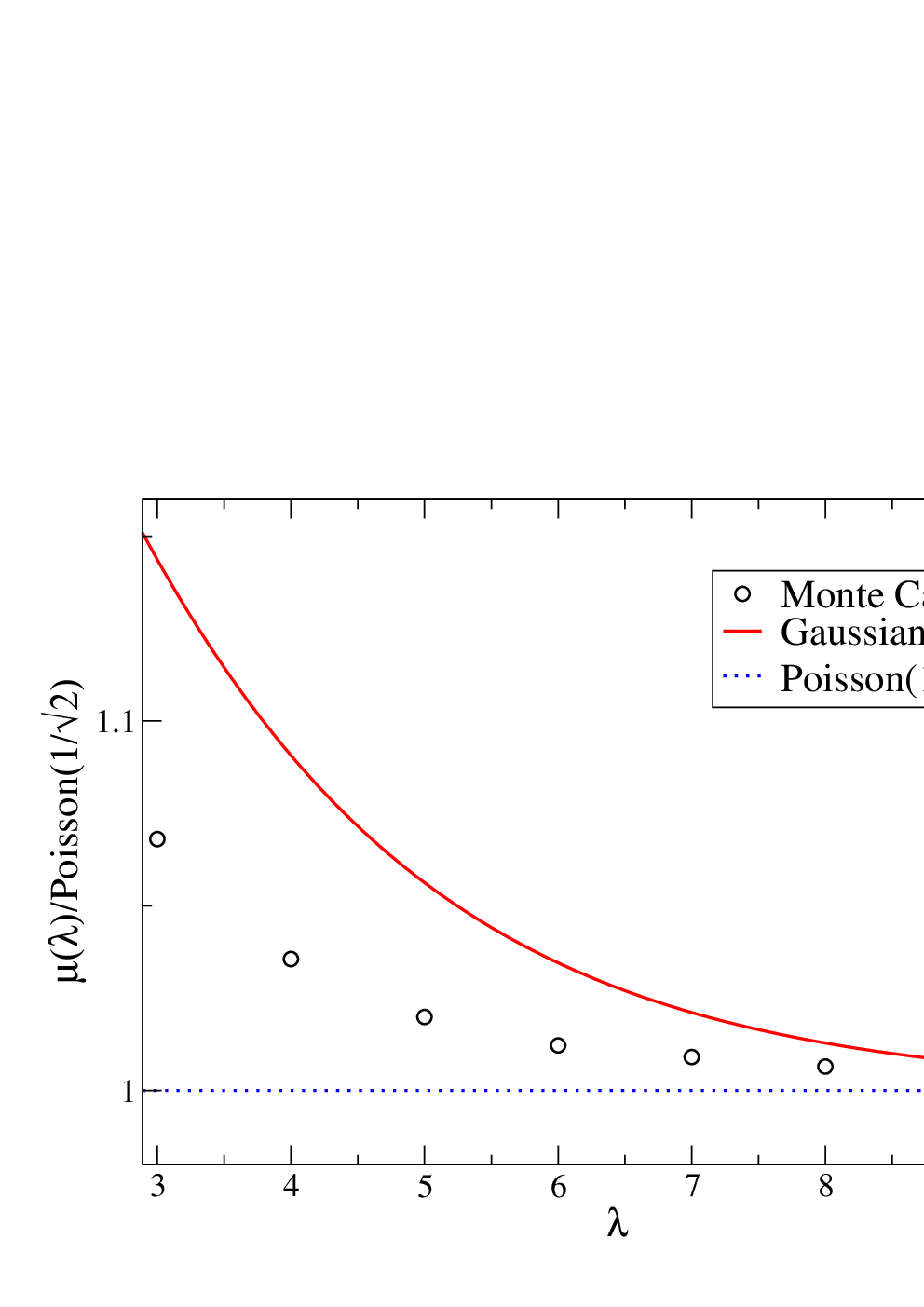
In the case of the hard-sphere model, a measurement of the largest eigenvalue $\mu(\lambda)$ is shown in Fig. 5. One can see that the numerical results are in very good agreement both with the Gaussian and the Sonine approximations. Figure 6 shows the large $\lambda$ behavior of $\mu(\lambda)$ divided by the prediction (38). In this case, a good agreement between the numerical data and the theoretical predictions is found. In the framework of the above described Monte Carlo algorithm, it is also possible to measure the stationary velocity pdf $g({\bf v},t=\infty,\lambda)$ which is equal to the eigenfunction ${\tilde{f}}({\bf v},\lambda)$ associated with $\mu(\lambda)$. Hence one can also compare the analytical predictions for the temperature $T(\lambda)$ and for the Sonine coefficient $a_{2}(\lambda)$ with the Monte Carlo results, see Figs. 7 and 8. In Fig. 7, one can see the temperature $T(\lambda)$. Here the Gaussian approximation is already able to capture the general behavior of this “effective” temperature, and for small values of $\lambda$, the Sonine corrections compare very well with the simulation data. In Fig. 8, one can see the coefficient $a_{2}$ as a function of $\lambda$. As expected, for small values of $\lambda$ the expansion carried out in the previous section correctly describes the result of the simulations.

The most direct way to measure the large deviation function of the number of collisions ${\cal N}$ is of course to count it in a (numerical) experiment, and then construct its probability distribution function. To this end, we have performed Molecular Dynamics (MD) simulations of a two dimensional hard-disk gas of $N=10^{3}$ particles of diameter $\sigma=1$ at density $\rho=N/V=10^{-3}\sigma^{-2}$ and $10^{-2}\sigma^{-2}$. The particles evolve in a square box with periodic boundary conditions, and the time is measured in mean free time units, in such a way that $\langle{\cal N}\rangle=t$. We measured the statistics of the number of collisions ${\cal N}$ suffered by each particle. The value of the first cumulants is reported in Table 1, together with the Poisson prediction, as well as the results from the Gaussian and Sonine approximations. It seems that, when time increases, the cumulants converge towards a value which is close to the Sonine predictions. However, it must be noted that even if increasing time makes finite time corrections smaller, the statistics become poorer and poorer. The agreement with the results from the Sonine approximation is very good, while the Gaussian order already provides a reliable estimation. This is further shown in Figure 9, where two measurements of the large deviation function of the number of collisions for two different times, $t=10$ and $t=50$ (with $\sigma=1$ and $T_{0}=1$), are compared to the numerical inverse Legendre Transform of $\mu(\lambda)$ at Gaussian order (given by Eq. (43)). Here again, the Poisson prediction is distinctly off.

References

- [1] L. Lue, J. Chem. Phys. 122, 044513 (2005).
- [2] M. H. Ernst, Phys. Reports 78, 1 (1981).
- [3] F. Coppex, M. Droz, and E. Trizac, Phys. Rev. E 69, 011303 (2004).
- [4] P. Visco, F. van Wijland and E. Trizac, to appear in Journal of Physical Chemistry B, arXiv:0801.2728.
- [5] D. Enskog, Physik Z. 12, 56 (1911).
- [6] A. Puglisi, P. Visco, E. Trizac, and F. van Wijland, Phys. Rev. E 73, 021301 (2006).
- [7] M. Abramowitz and I. A. Stegun, Handbook of mathematical functions with formulas, graphs and mathematical tables (Dover, New York, 1972).
- [8] F. W. Wiegel and J. P. J. Michels, Chem. Phys. Lett. 40 (1976).
- [9] G. A. Bird, Molecular Gas Dynamics and the Direct Simulation of Gas Flows (Clarendon, Oxford, 1994).
- [10] P. M. Morse and H. Feshbach, Methods of Theoretical Physics (McGraw-Hill, New York, 1953).
- [11] S. Chapman and T. G. Cowling, The mathematical theory of nonuniform gases (Cambridge University Press, London, 1960).
- [12] C. Giardinà, J. Kurchan, and L. Peliti, Phys. Rev. Lett. 96, 120603 (2006).
- [13] E. Trizac, Phys. Rev. Lett. 88, 160601 (2002).
- [14] J. Piasecki, E. Trizac and M. Droz, Phys. Rev. E 66, 066111 (2002).
- [15] E. Trizac and P. L. Krapivsky, Phys. Rev. Lett. 91, 218302 (2003).
- [16] T. Pöschel and S. Luding editors, Granular Gases, Berlin, 2001, Springer, Lecture Notes in Physics 564.
- [17] S. Luding, in: T.A.S.K. Quarterly, Scientific Bulletin of Academic Computer Centre of the Technical University of Gdansk, 2 (3), 417 (1998).
- [18] I. Pagonabarraga, E. Trizac, T.P.C. van Noije and M.H. Ernst, Phys. Rev. E 65, 011303 (2001).
- [19] D. L. Blair and A. Kudrolli, Phys. Rev. E 67, 041301 (2003).
- [20] D. Paolotti, C. Cattuto, U. Marini Bettolo Marconi and A. Puglisi, Granular Matter 5, 75 (2003).
- [21] E. Falcon, S. Aumaître, P. Évesque, F. Palencia, C. Lecoutre-Chabot, S. Fauve, D. Beysens and Y. Garrabos, Europhys. Lett. 74, 830 (2006).
- [22] P. Visco, A. Puglisi, A. Barrat, E. Trizac and F. van Wijland, Europhys. Lett. 72, 55 (2005).
- [23] M. H. Ernst and E. M. Hendriks, Phys. Lett. A 70, 183 (1979).