跳到论文正文
W Papers独立论文阅读器 arXiv:0803.1263 论文正文 计算阅读时间 · 0%
引用这篇论文根据当前论文元数据生成,正式投稿前建议核对。


License: arXiv.org perpetual non-exclusive license
arXiv:0803.1263v1 [cond-mat.str-el] 08 Mar 2008

Kondo effect in single-molecule magnet transistors

Gabriel González Affiliation: NanoScience Technology Center, University of Central Florida, Orlando, FL 32826, USA, Affiliation: Department of Physics, University of Central Florida, P.O. Box 162385, Orlando, FL 32816-2385, USA    Michael N. Leuenberger Email: mleuenbe@mail.ucf.edu Affiliation: NanoScience Technology Center, University of Central Florida, Orlando, FL 32826, USA, Affiliation: Department of Physics, University of Central Florida, P.O. Box 162385, Orlando, FL 32816-2385, USA    Eduardo R. Mucciolo Email: mucciolo@physics.ucf.edu Affiliation: Department of Physics, University of Central Florida, P.O. Box 162385, Orlando, FL 32816-2385, USA
August 24, 2026
Abstract

We present a careful and thorough microscopic derivation of the Kondo Hamiltonian for single-molecule magnets (SMMs) transistors. When the molecule is strongly coupled to metallic leads, we show that by applying a transverse magnetic field it is possible to topologically induce or quench the Kondo effect in the conductance of a SMM with either an integer or a half-integer spin S>1/2S>1/2. This topological Kondo effect is due to the Berry phase interference between multiple quantum tunneling paths of the spin. We calculate the renormalized Berry phase oscillations of the two Kondo peaks as a function of the transverse magnetic field by means of the poor man’s scaling. In particular, we show that the Kondo exchange interaction between itinerant electrons in the leads and the SMM pseudo spin 1/2 depends crucially on the SMM spin selection rules for the addition and subtraction of an electron and can range from antiferromagnetic to ferromagnetic. We illustrate our findings with the SMM Ni4, which we propose as a possible candidate for the experimental observation of the conductance oscillations.

Keywords: 
Single molecule magnets, Kondo effect, Berry phase
pacs
72.10.Fk, 03.65.Vf, 75.45.+j, 75.50.Xx

I Introduction

Single-molecule magnets (SMMs), such as Mn12 (see Refs. 1, 2) and Fe8 (see Refs. 3, 4), have become the focus of intense research since experiments on bulk samples demonstrated the quantum tunneling of a single magnetic moment on a macroscopic scale. These molecules are characterized by a large total spin, a large magnetic anisotropy barrier, and anisotropy terms which allow the spin to tunnel through the barrier. Electronic transport through SMMs offers several unique features with potentially large impact on applications such as high-density magnetic storage as well as quantum computing.[5] Recent experiments have pointed out the importance of the interference between spin tunneling paths in molecules. For instance, measurements of the magnetization in bulk Fe8 have observed oscillations in the tunnel splitting Δm,−m\Delta_{m,-m} between states Sz=mS_{z}=m and −m-m as a function of a transverse magnetic field at temperatures between 0.050.05 K and 0.70.7 K (see Ref. 6). This effect can be explained by the interference between Berry phases associated to spin tunneling paths of opposite windings.[7, 8] Theoretically, a coherent spin-state path integral formulation is used to account for the coherence of the virtual states over which the spin tunnels, although the initial and final spin states do not retain their coherence.

A new approach to the study of SMMs opened up recently with the first observation of quantized electronic transport through an isolated Mn12 molecule.[9] One expects a rich interplay between quantum tunneling, phase coherence, and electronic correlations in the transport properties of SMMs. In fact, it has been argued that the Kondo effect would only be observable for SMMs with half-integer spin [10, 11] and therefore absent for SMMs such as Mn12, Fe8, and Ni4, where the spin is integer. Later, two of us showed that this is not the case:[12] Remarkably, a transverse magnetic field H⊥H_{\bot} can be tuned to topologically quench the two lowest levels of a full-integer spin SMM, making them degenerate. In fact, the same Berry-phase interference also affects transport for SMMs with half-integer spin: In that case, sweeping H⊥H_{\bot} will lead not to one but a series of Kondo resonances. In the case of SMMs, as we show below, the Berry phase oscillations of the tunnel splitting Δm0,m0′\Delta_{m_{0},m^{\prime}_{0}} of the uncharged single-molecule magnet (q=0q=0) for both full- and half-integer spins leads to oscillation of the Kondo effect as a function of H⊥H_{\bot}. This means that the Kondo effect is observable at zero bias for all values of the magnetic field H⊥,0H_{\bot,0} such that Δm0,m0′​(H⊥,0)=0\Delta_{m_{0},m^{\prime}_{0}}(H_{\bot,0})=0.

It is interesting to note that at a finite bias the Kondo effect in a quantum dot in the presence of a magnetic field can be restored by tuning the bias to e​V=±g​μB​H⊥eV=\pm g\mu_{B}H_{\bot} (see Ref. 13). For SMMs, however, the interference between the Berry phases of the molecule total spin makes the distance between the split Kondo peaks, which is equal to e​V=±Δm0,m0′eV=\pm\Delta_{m_{0},m^{\prime}_{0}}, oscillate as a function of H⊥H_{\bot}. A necessary condition for observing these oscillations is a large enough tunnel splitting. Recently a new SMM based on tetranuclear nickel clusters Ni4 with a S=4S=4 ground state has been synthesized. [14] Our motivation for studying this particular nanomagnet stems partly from its high symmetry (S4)(S_{4}) but, more importantly, from the large tunnel splittings: Δm0,−m0∼0.01\Delta_{m_{0},-m_{0}}\sim 0.01 K or larger (depending on the transverse field H⊥H_{\bot}) between the |m⟩=|4⟩|m\rangle=|4\rangle and |m′⟩=|−4⟩|m^{\prime}\rangle=|-4\rangle ground states.

Recently, some authors have argued that the Kondo effect is absent at the diabolic points of the Berry-phase interference.[11] This conclusion came from considering an ad hoc Kondo Hamiltonian [10, 11] which was not derived microscopically. Moreover, in recent analysis of the sequential tunneling regime, an ad hoc exchange Hamiltonian mixed with an Anderson-type Hamiltonian was also used without a proper microscopic derivation.[15] In this paper, we provide a careful microscopic derivation of the Kondo Hamiltonian suitable for full- and half-integer spin single-molecule magnets by means of a Schrieffer-Wolff transformation.[16] By using the exact eigenstates of the positively and negatively charged single-molecule magnet, it is sufficient to apply the Schrieffer-Wolff transformation to second order in the tunneling matrix element. The resulting Kondo exchange parameters exhibit the interference between the second-order transition paths going over the two virtual charged states. We show that this very same interference phenomenon is also responsible for the Berry-phase blockade of the current through the single-molecule magnet in the cotunneling regime, which extends our previous results obtained for the Berry-phase blockade in the sequential tunneling regime.[17]

Our derivation of the Kondo Hamiltonian reveals an important detail: The Anderson-type Hamiltonian of the single-molecule magnet can be mapped onto a spin-1/2 Kondo Hamiltonian in two different ways: Let Sq=0S_{q=0} be the total spin of the uncharged single-molecule magnet.

  1. 1.

    If the total spins Sq=1S_{q=1} and Sq=−1S_{q=-1} in the ground state of the positively (q=−1q=-1) and negatively (q=1q=1) charged single-molecule magnet are equal to Sq=±1=Sq=0−1/2S_{q=\pm 1}=S_{q=0}-1/2, then the Kondo Hamiltonian exhibits an antiferromagnetic exchange coupling, which corresponds to the Kondo problem for spin 1/2 impurities or spin 1/2 quantum dots.

  2. 2.

    If Sq=±1=Sq=0+1/2S_{q=\pm 1}=S_{q=0}+1/2, then the Kondo Hamiltonian exhibits a ferromagnetic exchange coupling that leads to a vanishing renormalized transverse exchange coupling (Ising interaction), in which case the Kondo effect is absent.[18]

This point is at the very heart of the Kondo problem. The Kondo effect depends crucially on the selection rules for the addition and subtraction of a spin on the molecule. This result is in contrast to the Kondo effect seen in lateral quantum dots where the exchange coupling is always antiferromagnetic due to fact that spin states are degenerate in the absence of anisotropies.[19]

In the following, we provide a complete and detailed description of the Kondo effect in SMMs. Starting from a microscopic model (Sec. II), we derive the effective Kondo Hamiltonian for a SMM attached to metallic leads through tunneling barriers (Sec. III). In Sec. IV, we derive expressions for the conductance through a SMM for both zero and finite bias as a function of a transverse magnetic field and use the new SMM Ni4 to comment the experimental significance of our theoretical results. Our conclusions are summarized in Sec. VI.

II Microscopic Hamiltonian

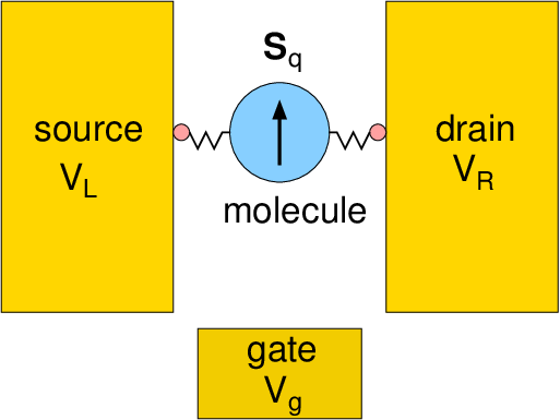
The total Anderson-impurity-like Hamiltonian of a system formed by a single-molecule magnet (SMM) attached to two metallic leads can be separated into three terms (see Fig. 1),

ℋtot=ℋSMM+ℋlead+ℋSMM−lead.{\cal H}_{\rm tot}={\cal H}_{\rm SMM}+{\cal H}_{\rm lead}+{\cal H}_{\rm SMM-lead}. (1)

The first term on the right-hand side of Eq. (1) denotes the SMM part, which can be broken into spin, orbital, charging, and gate contributions,

ℋSMM=ℋspin(q)+ℋorbital+q22​U−q​e​Vg,{\cal H}_{\rm SMM}={\cal H}_{\rm spin}^{(q)}+{\cal H}_{\rm orbital}+\frac{q^{2}}{2}\,U-q\,eV_{g}, (2)

where UU denotes the charging energy, qq is the number of excess electrons (the charge state of the molecule), and VgV_{g} is the electric potential due to an external gate voltage.[20] In the presence of an external magnetic field, the spin Hamiltonian of the SMM reads

ℋspin(q)\displaystyle{\cal H}_{\rm spin}^{(q)} =\displaystyle= −Aq​Sq,z2+B2,q2​(Sq,+2+Sq,−2)\displaystyle-A_{q}S_{q,z}^{2}+\frac{B_{2,q}}{2}\left(S_{q,+}^{2}+S_{q,-}^{2}\right) (3)
+B4,q3​(Sq,+4+Sq,−4)\displaystyle+\frac{B_{4,q}}{3}\left(S_{q,+}^{4}+S_{q,-}^{4}\right)
+12​(h⊥∗​Sq,++h⊥​Sq,−)+h∥​Sq,z,\displaystyle+\frac{1}{2}\left(h_{\bot}^{\ast}S_{q,+}+h_{\bot}S_{q,-}\right)+h_{\parallel}S_{q,z},

where the easy axis is taken along the zz direction and Sq,±=Sq,x±i​Sq,yS_{q,\pm}=S_{q,x}\pm iS_{q,y}. The magnetic field components were rescaled to h⊥=g​μB​(Hx+i​Hy)h_{\bot}=g\mu_{B}(H_{x}+iH_{y}) and h∥=g​μB​Hzh_{\parallel}=g\mu_{B}H_{z} for the transversal and longitudinal parts, respectively, where gg denotes the electron gyromagnetic factor. Note that the transverse magnetic field lies in the x​yxy plane. In this Hamiltonian, the dominant longitudinal anisotropy term creates a ladder structure in the molecule spectrum where the |±mq⟩|\pm m_{q}\rangle eigenstates of Sq,zS_{q,z} are degenerate. The weak transverse anisotropy terms couple these states. The total spin as well as the coupling parameters depend on the charging state of the molecule. For example, it is known that Mn12 changes its easy-axis anisotropy constant (and its total spin) from A0=56A_{0}=56 μ\mueV (Sq=0=10S_{q=0}=10) to A−1=43A_{-1}=43 μ\mueV (Sq=1=19/2S_{q=1}=19/2) and A−2=32A_{-2}=32 μ\mueV (Sq=2=10S_{q=2}=10) when singly and doubly charged, respectively.[21]
Refer to caption
Figure 1: (Color online) Schematic illustration of a single-molecule field-effect transistor formed by a single-molecule magnet attached to two metallic leads (source and drain) and controlled by a back gate voltage.

The orbital contribution to the SMM energy is given by

ℋorbital=∑n,σεn​σ​ψn​σ†​ψn​σ,{\cal H}_{\rm orbital}=\sum_{n,\sigma}\varepsilon_{n\sigma}\psi^{\dagger}_{n\sigma}\psi_{n\sigma}, (4)

where ψn​σ†\psi^{\dagger}_{n\sigma} (ψn​σ\psi_{n\sigma}) creates (annihilates) electrons in the molecular orbital state nn with spin orientation σ\sigma and energy εn​σ\varepsilon_{n\sigma}. Here we neglect any diamagnetic response to external magnetic fields.

The second and third terms on the right-hand side of Eq. (1) read, respectively,

ℋlead\displaystyle{\cal H}_{\rm lead} =\displaystyle= ∑a,k,σ[ξk(a)+12​(h⊥∗​𝐬a,++h⊥​𝐬a,−)+h∥​𝐬a,z]\displaystyle\sum_{a,k,\sigma}\left[\xi_{k}^{(a)}+\frac{1}{2}\left(h_{\bot}^{\ast}{\bf s}_{a,+}+h_{\bot}{\bf s}_{a,-}\right)+h_{\parallel}{\bf s}_{a,z}\right] (5)
×ψk​σ,a†​ψk​σ,a\displaystyle\times\psi_{k\sigma,a}^{\dagger}\psi_{k\sigma,a}

and

ℋSMM−lead=−∑a,k,σ,n[tn,k(a)ψk​σ,a†ψn​σ+H.c.],{\cal H}_{\rm SMM-lead}=-\sum_{a,k,\sigma,n}\left[t_{n,k}^{(a)}\psi^{\dagger}_{k\sigma,a}\psi_{n\sigma}+{\rm H.c.}\right], (6)

where 𝐬a=∑k,k′,σ,σ′∑a=R,Lψk​σ,a†​(σσ​σ′/2)​ψk′​σ′,a{\bf s}_{a}=\sum_{k,k^{\prime},\sigma,\sigma^{\prime}}\sum_{a=R,L}\psi_{k\sigma,a}^{\dagger}({\bf\sigma}_{\sigma\sigma^{\prime}}/2)\psi_{k^{\prime}\sigma^{\prime},a} and tn,k(a)t_{n,k}^{(a)} is the lead-molecule tunneling amplitude. The operator ψk​σ,a†\psi_{k\sigma,a}^{\dagger} (ψk​σ,a\psi_{k\sigma,a}) creates (annihilates) electronic states in the aa lead (a=R,La=R,L) with linear momentum kk, spin orientation σ\sigma, and energy ξk(a)\xi_{k}^{(a)}.

III The Kondo Hamiltonian

The weak tunneling amplitudes between the leads and the molecule and the large charging energy cause an effective exchange interaction between electrons in the leads and the spin of the molecule. Although this interaction at first glance seems to have the familiar Kondo ss-dd form, it is actually unusual because the transversal coupling involves only a subspace of the spin of the molecule. Below, we use perturbation theory to carefully derive an expression for the effective Kondo Hamiltonian of a SMM.

We begin by considering only the SMM and SMM-lead terms in Eq. (1). We divide the Hilbert space into subspaces corresponding to distinct charge sectors of the SMM. Using a block matrix representation, we have

ℋSMM+ℋSMM−lead=(⋱ℋq−1𝒱0𝒱†ℋq𝒲0𝒲†ℋq+1⋱),{\cal H}_{\rm SMM}+{\cal H}_{\rm SMM-lead}=\left(\begin{array}[]{ccccc}\ddots&&&&\\ &{\cal H}_{q-1}&{\cal V}&0&\\ &{\cal V}^{\dagger}&{\cal H}_{q}&{\cal W}&\\ &0&{\cal W}^{\dagger}&{\cal H}_{q+1}&\\ &&&&\ddots\end{array}\right), (7)

where ℋq{\cal H}_{q} is the SMM Hamiltonian for the charge sector qq [see Eq. (2)], while 𝒱{\cal V} and 𝒲{\cal W} represent the lead-SMM tunneling Hamiltonian, Eq. (6). For certain values of the gate voltage, the charging energy is compensated and Coulomb blockade is lifted. Away from these resonant points, there is an energy gap of order UU between consecutive diagonal elements in Eq. (7). Since U≫|tn,k|U\gg|t_{n,k}|, we can assume that the off-diagonal elements 𝒱{\cal V} and 𝒲{\cal W} are small perturbations and use a Schrieffer-Wolff transformation to decouple distinct charge sectors up to terms of order O⁡(|tn,k|2/U2)O(|t_{n,k}|^{2}/U^{2}).[16]

For simplicity, let us consider the sectors q=−1,0,+1q=-1,0,+1 only, where qq denotes the number of excess electrons, and write[22]

ℋ=𝒜+ℬ,{\cal H}={\cal A}+{\cal B}, (8)

where

𝒜=(ℋ−1000ℋ0000ℋ+1),ℬ=(0𝒱0𝒱†0𝒲0𝒲†0).{\cal A}=\left(\begin{array}[]{ccc}{\cal H}_{-1}&0&0\\ 0&{\cal H}_{0}&0\\ 0&0&{\cal H}_{+1}\end{array}\right),\ {\cal B}=\left(\begin{array}[]{ccc}0&{\cal V}&0\\ {\cal V}^{\dagger}&0&{\cal W}\\ 0&{\cal W}^{\dagger}&0\end{array}\right). (9)

Using the similarity transformation ℋ~=e𝒯​ℋ​e−𝒯\tilde{\cal H}=e^{{\cal T}}{\cal H}\,e^{-\cal T}, where 𝒯{\cal T} is anti-Hermitian, we have

ℋ~=ℋ+[𝒯,ℋ]+12​[𝒯,[𝒯,ℋ]]+⋯.\tilde{\cal H}={\cal H}+[{\cal T},{\cal H}]+\frac{1}{2}\left[{\cal T},[{\cal T},{\cal H}]\right]+\cdots. (10)

We want to determine 𝒯{\cal T} such that ℬ+[𝒯,𝒜]=0{\cal B}+[{\cal T},{\cal A}]=0. For that purpose, it is sufficient to assume that TT has the form

𝒯=(0𝒞0−𝒞†0𝒟0−𝒟†0),{\cal T}=\left(\begin{array}[]{ccc}0&{\cal C}&0\\ -{\cal C}^{\dagger}&0&{\cal D}\\ 0&-{\cal D}^{\dagger}&0\end{array}\right), (11)

with 𝒞{\cal C} and 𝒟{\cal D} satisfying

ℋ−1​𝒞−𝒞ℋ0=𝒱{\cal H}_{-1}{\cal C}-{\cal C}{\cal H}_{0}={\cal V} (12)

and

ℋ0​𝒟−𝒟ℋ+1=𝒲,{\cal H}_{0}{\cal D}-{\cal D}{\cal H}_{+1}={\cal W}, (13)

respectively. Thus,

ℋ~=𝒜+12​[𝒯,ℬ]+O⁡(ℬ3),\tilde{\cal H}={\cal A}+\frac{1}{2}[{\cal T},{\cal B}]+O({\cal B}^{3}), (14)

where

[𝒯,ℬ]=(𝒞𝒱†+𝒱𝒞†0𝒞𝒲−𝒱𝒟0𝒟𝒲†+𝒲𝒟†−𝒞†​𝒱−𝒱†​𝒞0𝒲†​𝒞†−𝒟†​𝒱†0−𝒟†​𝒲−𝒲†​𝒟.).[{\cal T},{\cal B}]=\left(\begin{array}[]{ccc}{\cal C}{\cal V}^{\dagger}+{\cal V}{\cal C}^{\dagger}&0&{\cal C}{\cal W}-{\cal V}{\cal D}\\ 0&{\cal D}{\cal W}^{\dagger}+{\cal W}{\cal D}^{\dagger}-{\cal C}^{\dagger}{\cal V}-{\cal V}^{\dagger}{\cal C}&0\\ {\cal W}^{\dagger}{\cal C}^{\dagger}-{\cal D}^{\dagger}{\cal V}^{\dagger}&0&-{\cal D}^{\dagger}{\cal W}-{\cal W}^{\dagger}{\cal D}.\end{array}\right). (15)

Note that the neutral sector (q=0q=0) has been decoupled from the charged sectors at the expense of adding two contributions of order O​(𝒱,𝒲)2O({\cal V,W})^{2} to ℋ0{\cal H}_{0}. To specify the form of these contributions, we use the eigenbasis {|α⟩q}\{|\alpha\rangle_{q}\} of ℋq{\cal H}_{q}, namely,

⟨α|ℋq|β⟩qq=[ℋq]α​β=δα,βEα(q).{{}_{q}}\langle\alpha|{\cal H}_{q}|\beta\rangle_{q}=[{\cal H}_{q}]_{\alpha\beta}=\delta_{\alpha,\beta}\,E^{(q)}_{\alpha}. (16)

Equations (12) and (13) can be solved in this representation to yield

⟨α|𝒞|β⟩0−1=[𝒞]α​β=[𝒱]α​βEα(−1)−Eβ(0){{}_{-1}}\langle\alpha|{\cal C}|\beta\rangle_{0}=[{\cal C}]_{\alpha\beta}=\frac{[{\cal V}]_{\alpha\beta}}{E_{\alpha}^{(-1)}-E_{\beta}^{(0)}} (17)

and

⟨α|𝒟|β⟩+10=[𝒟]α​β=[𝒲]α​βEα(0)−Eβ(+1),{{}_{0}}\langle\alpha|{\cal D}|\beta\rangle_{+1}=[{\cal D}]_{\alpha\beta}=\frac{[{\cal W}]_{\alpha\beta}}{E_{\alpha}^{(0)}-E_{\beta}^{(+1)}}, (18)

respectively, where [𝒱]α​β=⟨α|𝒱|β⟩0−1[{\cal V}]_{\alpha\beta}=\left.{{}_{-1}}\langle\alpha|{\cal V}|\beta\rangle_{0}\right. and [𝒲]α​β=⟨α|𝒲|β⟩−10[{\cal W}]_{\alpha\beta}=\left.{{}_{0}}\langle\alpha|{\cal W}|\beta\rangle_{-1}\right.. This allows us to write the following matrix elements for the neutral sector:

⟨α|𝒟𝒲†|β⟩00=∑γ[𝒲]α​γ​[𝒲†]γ​βEα(0)−Eγ(+1){{}_{0}}\langle\alpha|{\cal D}{\cal W}^{\dagger}|\beta\rangle_{0}=\sum_{\gamma}\frac{[{\cal W}]_{\alpha\gamma}[{\cal W}^{\dagger}]_{\gamma\beta}}{E_{\alpha}^{(0)}-E_{\gamma}^{(+1)}} (19)

and

⟨α|𝒱†𝒞|β⟩00=∑γ[𝒱†]α​γ​[𝒱]γ​βEγ(−1)−Eβ(0).{{}_{0}}\langle\alpha|{\cal V}^{\dagger}{\cal C}|\beta\rangle_{0}=\sum_{\gamma}\frac{[{\cal V}^{\dagger}]_{\alpha\gamma}[{\cal V}]_{\gamma\beta}}{E_{\gamma}^{(-1)}-E_{\beta}^{(0)}}. (20)
Refer to caption
Figure 2: (Color online) Energy spectra of consecutive charging sectors of the SMM Hamiltonian (q=−1,0,1q=-1,0,1). Δq≡Δmq,−mq\Delta_{q}\equiv\Delta_{m_{q},-m_{q}} is the tunnel splitting due to the in-plane anisotropy and Es/a,mq(q)E^{(q)}_{{\rm s/a},m_{q}} denote energy eigenstates corresponding to symmetric and antisymmetric combinations of the ground eigenstates |±sq⟩|\pm s_{q}\rangle of the longitudinal component of the SMM total spin Sq,zS_{q,z}.

In the Coulomb blockade valley, when Vg=0V_{g}=0 in Eq. (2), the eigenstates of the Hamiltonian ℋq{\cal H}_{q} are expressed in terms of symmetric and antisymmetric combinations of the eigenstates of the Sq,zS_{q,z} operator, namely,

|s,a⟩mq=12[|mq⟩0±|−mq⟩0],|{\rm s,a}\rangle_{m_{q}}=\frac{1}{\sqrt{2}}\left[|m_{q}\rangle_{0}\pm|-m_{q}\rangle_{0}\right], (21)

with mq=0,1,2,…,Sqm_{q}=0,1,2,\ldots,S_{q} if SqS_{q} is integer and mq=12,32,…,Sqm_{q}=\frac{1}{2},\frac{3}{2},\ldots,S_{q} if SqS_{q} is half-integer.[23] Note that since the matrices 𝒲{\cal W} and 𝒱{\cal V} represent the addition (subtraction) of an electron to (from) the SMM, only q=0q=0 states that differ in spin projection by 11 are coupled through Eqs. (19) and (20). Conservation of angular momentum upon electron tunneling requires that the intermediate states in the q=1q=1 or q=−1q=-1 sectors obey |S±1−S0|=1/2|S_{\pm 1}-S_{0}|=1/2. For instance, when the SMM total spin is lowered by the addition or subtraction of an electron, longitudinal spin components satisfy m±1=S±1=S0−1/2m_{\pm 1}=S_{\pm 1}=S_{0}-1/2 and −m±1=−S±1=−S0+1/2-m_{\pm 1}=-S_{\pm 1}=-S_{0}+1/2. Therefore, we define the spin states of the ground state to be |↑q⟩=|mq⟩\left|\uparrow_{q}\right>=\left|m_{q}\right> and |↓q⟩=|−mq⟩\left|\downarrow_{q}\right>=\left|-m_{q}\right>. The corresponding eigenenergies are represented in Fig. 2.

Let us first consider intermediate states involving the q=1q=1 sector. This situation corresponds to a small positive gate voltage (Vg>0V_{g}>0). Equation (19) can be used to write the matrix elements of the reduced Hamiltonian of the q=0q=0 sector in terms of a product of energy denominators and matrix elements of 𝒲{\cal W}. Using the {|↑⟩q,|↓⟩q}\{|\uparrow\rangle_{q},|\downarrow\rangle_{q}\} basis and inserting complete eigenvector sets for each sector, i.e. ℐ(q)=|s⟩q⟨s|+|a⟩qq⟨a|q{\cal I}^{(q)}=|s\rangle_{q}{{}_{q}}\langle s|+|a\rangle_{q}{{}_{q}}\langle a|, we find

⟨↑|𝒟𝒲†+𝒲𝒟†|↑⟩00\displaystyle{{}_{0}}\langle\uparrow|{\cal D}{\cal W}^{\dagger}+{\cal W}{\cal D}^{\dagger}|\uparrow\rangle_{0} =\displaystyle= ⟨↑|s⟩00⟨s|𝒟|s⟩10⟨s|𝒲†|↑⟩01+⟨↑|a⟩00⟨a|𝒟|s⟩10⟨s|𝒲†|↑⟩01\displaystyle{{}_{0}}\langle\uparrow|s\rangle_{0}{{}_{0}}\langle s|{\cal D}|s\rangle_{1}{{}_{1}}\langle s|{\cal W}^{\dagger}|\uparrow\rangle_{0}+\,{{}_{0}}\langle\uparrow|a\rangle_{0}{{}_{0}}\langle a|{\cal D}|s\rangle_{1}{{}_{1}}\langle s|{\cal W}^{\dagger}|\uparrow\rangle_{0} (22)
+⟨↑|s⟩00⟨s|𝒟|a⟩10⟨a|𝒲†|↑⟩01+⟨↑|a⟩00⟨a|𝒟|a⟩10⟨a|𝒲†|↑⟩01+H.c.,\displaystyle\left.\ +\,{{}_{0}}\langle\uparrow|s\rangle_{0}{{}_{0}}\langle s|{\cal D}|a\rangle_{1}{{}_{1}}\langle a|{\cal W}^{\dagger}|\uparrow\rangle_{0}+\,{{}_{0}}\langle\uparrow|a\rangle_{0}{{}_{0}}\langle a|{\cal D}|a\rangle_{1}{{}_{1}}\langle a|{\cal W}^{\dagger}|\uparrow\rangle_{0}+\,\mbox{H.c.},\right.
⟨↓|𝒟𝒲†+𝒲𝒟†|↓⟩00\displaystyle{{}_{0}}\langle\downarrow|{\cal D}{\cal W}^{\dagger}+{\cal W}{\cal D}^{\dagger}|\downarrow\rangle_{0} =\displaystyle= ⟨↓|s⟩00⟨s|𝒟|s⟩10⟨s|𝒲†|↓⟩01+⟨↓|a⟩00⟨a|𝒟|s⟩10⟨s|𝒲†|↓⟩01\displaystyle{{}_{0}}\langle\downarrow|s\rangle_{0}{{}_{0}}\langle s|{\cal D}|s\rangle_{1}{{}_{1}}\langle s|{\cal W}^{\dagger}|\downarrow\rangle_{0}+\,{{}_{0}}\langle\downarrow|a\rangle_{0}{{}_{0}}\langle a|{\cal D}|s\rangle_{1}{{}_{1}}\langle s|{\cal W}^{\dagger}|\downarrow\rangle_{0} (23)
+⟨↓|s⟩00⟨s|𝒟|a⟩10⟨a|𝒲†|↓⟩01+⟨↓|a⟩00⟨a|𝒟|a⟩10⟨a|𝒲†|↓⟩01+H.c.,\displaystyle\left.\ +\,{{}_{0}}\langle\downarrow|s\rangle_{0}{{}_{0}}\langle s|{\cal D}|a\rangle_{1}{{}_{1}}\langle a|{\cal W}^{\dagger}|\downarrow\rangle_{0}+\,{{}_{0}}\langle\downarrow|a\rangle_{0}{{}_{0}}\langle a|{\cal D}|a\rangle_{1}{{}_{1}}\langle a|{\cal W}^{\dagger}|\downarrow\rangle_{0}+\,\mbox{H.c.},\right.

and

⟨↑|𝒟𝒲†+𝒲𝒟†|↓⟩00\displaystyle{{}_{0}}\langle\uparrow|{\cal D}{\cal W}^{\dagger}+{\cal W}{\cal D}^{\dagger}|\downarrow\rangle_{0} =\displaystyle= ⟨↑|𝒟𝒲†|↓⟩00+(⟨↓|𝒟𝒲†|↑⟩00)†,\displaystyle{{}_{0}}\langle\uparrow|{\cal D}{\cal W}^{\dagger}|\downarrow\rangle_{0}+\left({{}_{0}}\langle\downarrow|{\cal D}{\cal W}^{\dagger}|\uparrow\rangle_{0}\right)^{\dagger}, (24)

where

⟨↑|𝒟𝒲†|↓⟩00\displaystyle{{}_{0}}\langle\uparrow|{\cal D}{\cal W}^{\dagger}|\downarrow\rangle_{0} =\displaystyle= ⟨↑|s⟩00⟨s|𝒟|s⟩10⟨s|𝒲†|↓⟩01+⟨↑|a⟩00⟨a|𝒟|a⟩10⟨a|𝒲†|↓⟩01\displaystyle{{}_{0}}\langle\uparrow|s\rangle_{0}{{}_{0}}\langle s|{\cal D}|s\rangle_{1}{{}_{1}}\langle s|{\cal W}^{\dagger}|\downarrow\rangle_{0}+\,{{}_{0}}\langle\uparrow|a\rangle_{0}{{}_{0}}\langle a|{\cal D}|a\rangle_{1}{{}_{1}}\langle a|{\cal W}^{\dagger}|\downarrow\rangle_{0} (25)
+⟨↑|s⟩00⟨s|𝒟|a⟩10⟨a|𝒲†|↓⟩01+⟨↑|a⟩00⟨a|𝒟|s⟩10⟨s|𝒲†|↓⟩01,\displaystyle\left.\ +\,{{}_{0}}\langle\uparrow|s\rangle_{0}{{}_{0}}\langle s|{\cal D}|a\rangle_{1}{{}_{1}}\langle a|{\cal W}^{\dagger}|\downarrow\rangle_{0}+\,{{}_{0}}\langle\uparrow|a\rangle_{0}{{}_{0}}\langle a|{\cal D}|s\rangle_{1}{{}_{1}}\langle s|{\cal W}^{\dagger}|\downarrow\rangle_{0},\right.

and

⟨↓|𝒟𝒲†|↑⟩00\displaystyle{{}_{0}}\langle\downarrow|{\cal D}{\cal W}^{\dagger}|\uparrow\rangle_{0} =\displaystyle= ⟨↓|s⟩00⟨s|𝒟|s⟩10⟨s|𝒲†|↑⟩01+⟨↓|a⟩00⟨a|𝒟|s⟩10⟨s|𝒲†|↑⟩01\displaystyle{{}_{0}}\langle\downarrow|s\rangle_{0}{{}_{0}}\langle s|{\cal D}|s\rangle_{1}{{}_{1}}\langle s|{\cal W}^{\dagger}|\uparrow\rangle_{0}+\,{{}_{0}}\langle\downarrow|a\rangle_{0}{{}_{0}}\langle a|{\cal D}|s\rangle_{1}{{}_{1}}\langle s|{\cal W}^{\dagger}|\uparrow\rangle_{0} (26)
+⟨↓|s⟩00⟨s|𝒟|a⟩10⟨a|𝒲†|↑⟩01+⟨↓|a⟩00⟨a|𝒟|a⟩10⟨a|𝒲†|↑⟩01.\displaystyle\left.\ +\,{{}_{0}}\langle\downarrow|s\rangle_{0}{{}_{0}}\langle s|{\cal D}|a\rangle_{1}{{}_{1}}\langle a|{\cal W}^{\dagger}|\uparrow\rangle_{0}+\,{{}_{0}}\langle\downarrow|a\rangle_{0}{{}_{0}}\langle a|{\cal D}|a\rangle_{1}{{}_{1}}\langle a|{\cal W}^{\dagger}|\uparrow\rangle_{0}.\right.

Using Eq. (18) and the fact that Ea(+1)=Es(+1)+Δ1E_{a}^{(+1)}=E_{s}^{(+1)}+\Delta_{1}, ⟨↑|s⟩00=⟨↓|s⟩00=⟨↑|a⟩00=1/2{{}_{0}}\langle\uparrow|s\rangle_{0}=\,{{}_{0}}\langle\downarrow|s\rangle_{0}=\,{{}_{0}}\langle\uparrow|a\rangle_{0}=1/\sqrt{2}, and ⟨↓|a⟩00=−1/2{{}_{0}}\langle\downarrow|a\rangle_{0}=-1/\sqrt{2}, we find, after some algebra,

⟨↑|𝒟𝒲†+𝒲𝒟†|↑⟩00\displaystyle{{}_{0}}\langle\uparrow|{\cal D}{\cal W}^{\dagger}+{\cal W}{\cal D}^{\dagger}|\uparrow\rangle_{0} =\displaystyle= 12​Δs​Δs​a[⟨s|(Δs𝒲ℐ(1)𝒲†−Δ1𝒲|s⟩1⟨s|𝒲†)1|↑⟩00]\displaystyle\frac{1}{\sqrt{2}\Delta_{s}\Delta_{sa}}\left[{{}_{0}}\langle s|\left(\Delta_{s}{\cal W}{\cal I}^{(1)}{\cal W}^{\dagger}-\Delta_{1}{\cal W}|s\rangle_{1}{{}_{1}}\langle s|{\cal W}^{\dagger}\right)\ |\uparrow\rangle_{0}\right] (27)
+12​Δa​Δa​s[⟨a|(Δa​s𝒲ℐ(1)𝒲†−Δ1𝒲|s⟩1⟨s|𝒲†)1|↑⟩00]+H.c.,\displaystyle\left.\ +\,\frac{1}{\sqrt{2}\Delta_{a}\Delta_{as}}\left[{{}_{0}}\langle a|\left(\Delta_{as}{\cal W}{\cal I}^{(1)}{\cal W}^{\dagger}-\Delta_{1}{\cal W}|s\rangle_{1}{{}_{1}}\langle s|{\cal W}^{\dagger}\right)|\uparrow\rangle_{0}\right]+\mbox{H.c.},\right.
⟨↓|𝒟𝒲†+𝒲𝒟†|↓⟩00\displaystyle{{}_{0}}\langle\downarrow|{\cal D}{\cal W}^{\dagger}+{\cal W}{\cal D}^{\dagger}|\downarrow\rangle_{0} =\displaystyle= 12​Δs​Δs​a[⟨s|(Δs𝒲ℐ(1)𝒲†−Δ1𝒲|s⟩1⟨s|𝒲†)1|↓⟩00]\displaystyle\frac{1}{\sqrt{2}\Delta_{s}\Delta_{sa}}\left[{}_{0}\langle s|\left(\Delta_{s}{\cal W}{\cal I}^{(1)}{\cal W}^{\dagger}-\Delta_{1}{\cal W}|s\rangle_{1}{{}_{1}}\langle s|{\cal W}^{\dagger}\right)\ |\downarrow\rangle_{0}\right] (28)
−12​Δa​Δa​s[⟨a|(Δa​s𝒲ℐ(1)𝒲†−Δ1𝒲|s⟩1⟨s|𝒲†)1|↓⟩00]+H.c.,\displaystyle\left.\ -\,\frac{1}{\sqrt{2}\Delta_{a}\Delta_{as}}\left[{{}_{0}}\langle a|\left(\Delta_{as}{\cal W}{\cal I}^{(1)}{\cal W}^{\dagger}-\Delta_{1}{\cal W}|s\rangle_{1}{{}_{1}}\langle s|{\cal W}^{\dagger}\right)|\downarrow\rangle_{0}\right]+\mbox{H.c.},\right.
⟨↑|𝒟𝒲†|↓⟩00\displaystyle{{}_{0}}\langle\uparrow|{\cal D}{\cal W}^{\dagger}|\downarrow\rangle_{0} =\displaystyle= 12​Δs​Δs​a[⟨s|(Δs𝒲ℐ(1)𝒲†−Δ1𝒲|s⟩1⟨s|𝒲†)1|↓⟩00]\displaystyle\frac{1}{\sqrt{2}\Delta_{s}\Delta_{sa}}\left[{{}_{0}}\langle s|\left(\Delta_{s}{\cal W}{\cal I}^{(1)}{\cal W}^{\dagger}-\Delta_{1}{\cal W}|s\rangle_{1}{{}_{1}}\langle s|{\cal W}^{\dagger}\right)\ |\downarrow\rangle_{0}\right] (29)
+12​Δa​Δa​s[⟨a|(Δa​s𝒲ℐ(1)𝒲†−Δ1𝒲|s⟩1⟨s|𝒲†)1|↓⟩00],\displaystyle\left.\ +\,\frac{1}{\sqrt{2}\Delta_{a}\Delta_{as}}\left[{{}_{0}}\langle a|\left(\Delta_{as}{\cal W}{\cal I}^{(1)}{\cal W}^{\dagger}-\Delta_{1}{\cal W}|s\rangle_{1}{{}_{1}}\langle s|{\cal W}^{\dagger}\right)|\downarrow\rangle_{0}\right],\right.

and

⟨↓|𝒟𝒲†|↑⟩00\displaystyle{{}_{0}}\langle\downarrow|{\cal D}{\cal W}^{\dagger}|\uparrow\rangle_{0} =\displaystyle= 12​Δs​Δs​a[⟨s|(Δs𝒲ℐ(1)𝒲†−Δ1𝒲|s⟩1⟨s|𝒲†)1|↑⟩00]\displaystyle\frac{1}{\sqrt{2}\Delta_{s}\Delta_{sa}}\left[{{}_{0}}\langle s|\left(\Delta_{s}{\cal W}{\cal I}^{(1)}{\cal W}^{\dagger}-\Delta_{1}{\cal W}|s\rangle_{1}{{}_{1}}\langle s|{\cal W}^{\dagger}\right)\ |\uparrow\rangle_{0}\right] (30)
−12​Δa​Δa​s[⟨a|(Δa​s𝒲ℐ(1)𝒲†−Δ1𝒲|s⟩1⟨s|𝒲†)1|↑⟩00],\displaystyle\left.\ -\,\frac{1}{\sqrt{2}\Delta_{a}\Delta_{as}}\left[{{}_{0}}\langle a|\left(\Delta_{as}{\cal W}{\cal I}^{(1)}{\cal W}^{\dagger}-\Delta_{1}{\cal W}|s\rangle_{1}{{}_{1}}\langle s|{\cal W}^{\dagger}\right)|\uparrow\rangle_{0}\right],\right.

where Δs=Es(0)−Es(+1)\Delta_{s}=E_{s}^{(0)}-E_{s}^{(+1)}, Δs​a=Es(0)−Ea(+1)\Delta_{sa}=E_{s}^{(0)}-E_{a}^{(+1)}, Δa=Ea(0)−Ea(+1)\Delta_{a}=E_{a}^{(0)}-E_{a}^{(+1)}, and Δa​s=Ea(0)−Es(+1)\Delta_{as}=E_{a}^{(0)}-E_{s}^{(+1)}. To calculate the matrix elements in Eqs. (27), (23), (24), and (25) we use the following definition for the operator 𝒲{\cal W} that originates from the lead-SMM Hamiltonian in Eq. (6):

𝒲=−∑a,k,σ,ntn,k(a)ψ†k​σ,aψn​σ,{\cal W}=-\sum_{a,k,\sigma,n}t_{n,k}^{(a)}\,\psi^{\dagger}_{k\sigma,a}\psi_{n\sigma}, (31)

with nn being an occupied molecular orbital for a SMM in the charge state q=1q=1. Similarly, we define

𝒲†=∑a,k,σ,ntn,k(a)​ψk​σ,a​ψn​σ†,{\cal W}^{\dagger}=\sum_{a,k,\sigma,n}t_{n,k}^{(a)}\,\psi_{k\sigma,a}\psi_{n\sigma}^{\dagger}, (32)

which leads to

𝒲ℐ(1)𝒲†=−∑a,k,σ,n∑a′,k′,σ′,n′tn,k(a)tn′,k′(a′)ψk​σ,a†ψk′​σ′,a′(ψn​σℐ(1)ψn′​σ′†){\cal W}{\cal I}^{(1)}{\cal W}^{\dagger}=-\sum_{a,k,\sigma,n}\sum_{a^{\prime},k^{\prime},\sigma^{\prime},n^{\prime}}t_{n,k}^{(a)}t_{n^{\prime},k^{\prime}}^{(a^{\prime})}\psi^{\dagger}_{k\sigma,a}\psi_{k^{\prime}\sigma^{\prime},a^{\prime}}\left(\psi_{n\sigma}{\cal I}^{(1)}\psi_{n^{\prime}\sigma^{\prime}}^{\dagger}\right) (33)

and

𝒲|s⟩1⟨s|𝒲†=−∑a,k,σ,n∑a′,k′,σ′,n′tn,k(a)tn′,k′(a′)ψk​σ,a†ψk′​σ′,a′(ψn​σ|s⟩1⟨s|ψn′​σ′†)1.1{\cal W}|s\rangle_{1}{{}_{1}}\langle s|{\cal W}^{\dagger}=-\sum_{a,k,\sigma,n}\sum_{a^{\prime},k^{\prime},\sigma^{\prime},n^{\prime}}t_{n,k}^{(a)}t_{n^{\prime},k^{\prime}}^{(a^{\prime})}\psi^{\dagger}_{k\sigma,a}\psi_{k^{\prime}\sigma^{\prime},a^{\prime}}\left(\psi_{n\sigma}|s\rangle_{1}{{}_{1}}\langle s|\psi_{n^{\prime}\sigma^{\prime}}^{\dagger}\right). (34)

III.1 First set of spin selection rules

We will now consider the case when adding or subtracting an electron always decreases the SMM total spin, namely, Sq=±1=Sq=0−1/2S_{q=\pm 1}=S_{q=0}-1/2. This selection rule can be enforced through the adoption of the following matrix elements:

⟨↑|ψn​σ|↑⟩10=δm0,m1−σδσ,↓,{{}_{0}}\langle\uparrow|\psi_{n\sigma}|\uparrow\rangle_{1}=\delta_{m_{0},m_{1}-\sigma}\,\delta_{\sigma,\downarrow}, (35)
⟨↓|ψn​σ|↓⟩10=δ−m0,−m1−σδσ,↑,{{}_{0}}\langle\downarrow|\psi_{n\sigma}|\downarrow\rangle_{1}=\delta_{-m_{0},-m_{1}-\sigma}\,\delta_{\sigma,\uparrow}, (36)
⟨↑|ψn​σ†|↑⟩01=δm0,m1−σδσ,↓,{{}_{1}}\langle\uparrow|\psi_{n\sigma}^{\dagger}|\uparrow\rangle_{0}=\delta_{m_{0},m_{1}-\sigma}\,\delta_{\sigma,\downarrow}, (37)

and

⟨↓|ψn​σ†|↓⟩01=δ−m0,−m1−σδσ,↑,{{}_{1}}\langle\downarrow|\psi_{n\sigma}^{\dagger}|\downarrow\rangle_{0}=\delta_{-m_{0},-m_{1}-\sigma}\,\delta_{\sigma,\uparrow}, (38)

(For the sake of simplicity, we will assume that m0,m1>12m_{0},m_{1}>\frac{1}{2} and σ=±12\sigma=\pm\frac{1}{2} hereafter.) Then, substituting Eq. (33) and Eq. (34) into Eqs. (27), (23), (24) and (25), we arrive at

⟨↑|𝒟𝒲†+𝒲𝒟†|↑⟩00=−∑k,a,n∑k′,a′,n′Jk,a;k′,a′z⁡(+1)ψk↓,a†ψk′↓,a′−∑k,a,n∑k′,a′,n′jk,a;k′,a′⟂(+1)(ψk↑,a†ψk′↓,a′+ψk↓,a†ψk′↑,a′),{{}_{0}}\langle\uparrow|{\cal D}{\cal W}^{\dagger}+{\cal W}{\cal D}^{\dagger}|\uparrow\rangle_{0}=-\sum_{k,a,n}\sum_{k^{\prime},a^{\prime},n^{\prime}}J_{k,a;k^{\prime},a^{\prime}}^{z\,(+1)}\psi^{\dagger}_{k\downarrow,a}\psi_{k^{\prime}\downarrow,a^{\prime}}\,-\sum_{k,a,n}\sum_{k^{\prime},a^{\prime},n^{\prime}}j_{k,a;k^{\prime},a^{\prime}}^{\perp\,(+1)}\left(\psi^{\dagger}_{k\uparrow,a}\psi_{k^{\prime}\downarrow,a^{\prime}}+\psi^{\dagger}_{k\downarrow,a}\psi_{k^{\prime}\uparrow,a^{\prime}}\right), (39)
⟨↓|𝒟𝒲†+𝒲𝒟†|↓⟩00=−∑k,a,n∑k′,a′,n′Jk,a;k′,a′z⁡(+1)ψk↑,a†ψk′↑,a′−∑k,a,n∑k′,a′,n′jk,a;k′,a′⟂(+1)(ψk↑,a†ψk′↓,a′+ψk↓,a†ψk′↑,a′),{{}_{0}}\langle\downarrow|{\cal D}{\cal W}^{\dagger}+{\cal W}{\cal D}^{\dagger}|\downarrow\rangle_{0}=-\sum_{k,a,n}\sum_{k^{\prime},a^{\prime},n^{\prime}}J_{k,a;k^{\prime},a^{\prime}}^{z\,(+1)}\psi^{\dagger}_{k\uparrow,a}\psi_{k^{\prime}\uparrow,a^{\prime}}\,-\sum_{k,a,n}\sum_{k^{\prime},a^{\prime},n^{\prime}}j_{k,a;k^{\prime},a^{\prime}}^{\perp\,(+1)}\left(\psi^{\dagger}_{k\uparrow,a}\psi_{k^{\prime}\downarrow,a^{\prime}}+\psi^{\dagger}_{k\downarrow,a}\psi_{k^{\prime}\uparrow,a^{\prime}}\right), (40)
⟨↑|𝒟𝒲†+𝒲𝒟†|↓⟩00=−∑k,a,n∑k′,a′,n′Jk,a;k′,a′⟂(+1)ψk↓,a†ψk′↑,a′−∑k,a,n∑k′,a′,n′jk,a;k′,a′z⁡(+1)(ψk↑,a†ψk′↑,a′+ψk↓,a†ψk′↓,a′),\displaystyle{{}_{0}}\langle\uparrow|{\cal D}{\cal W}^{\dagger}+{\cal W}{\cal D}^{\dagger}|\downarrow\rangle_{0}=-\sum_{k,a,n}\sum_{k^{\prime},a^{\prime},n^{\prime}}J_{k,a;k^{\prime},a^{\prime}}^{\perp\,(+1)}\psi^{\dagger}_{k\downarrow,a}\psi_{k^{\prime}\uparrow,a^{\prime}}\,-\sum_{k,a,n}\sum_{k^{\prime},a^{\prime},n^{\prime}}j_{k,a;k^{\prime},a^{\prime}}^{z\,(+1)}\left(\psi^{\dagger}_{k\uparrow,a}\psi_{k^{\prime}\uparrow,a^{\prime}}+\psi^{\dagger}_{k\downarrow,a}\psi_{k^{\prime}\downarrow,a^{\prime}}\right), (41)

and

⟨↓|𝒟𝒲†+𝒲𝒟†|↑⟩00=−∑k,a,n∑k′,a′,n′Jk,a;k′,a′⟂(+1)ψk↑,a†ψk′↓,a′−∑k,a,n∑k′,a′,n′jk,a;k′,a′z⁡(+1)(ψk↑,a†ψk′↑,a′+ψk↓,a†ψk′↓,a′).\displaystyle{{}_{0}}\langle\downarrow|{\cal D}{\cal W}^{\dagger}+{\cal W}{\cal D}^{\dagger}|\uparrow\rangle_{0}=-\sum_{k,a,n}\sum_{k^{\prime},a^{\prime},n^{\prime}}J_{k,a;k^{\prime},a^{\prime}}^{\perp\,(+1)}\psi^{\dagger}_{k\uparrow,a}\psi_{k^{\prime}\downarrow,a^{\prime}}\,-\sum_{k,a,n}\sum_{k^{\prime},a^{\prime},n^{\prime}}j_{k,a;k^{\prime},a^{\prime}}^{z\,(+1)}\left(\psi^{\dagger}_{k\uparrow,a}\psi_{k^{\prime}\uparrow,a^{\prime}}+\psi^{\dagger}_{k\downarrow,a}\psi_{k^{\prime}\downarrow,a^{\prime}}\right). (42)

Using a similar procedure, we also find

⟨↑|𝒞†𝒱+𝒱†𝒞|↑⟩00=∑k,a,n∑k′,a′,n′Jk,a;k′,a′z⁡(−1)ψk′↑,a′ψk↑,a†+∑k,a,n∑k′,a′,n′jk,a;k′,a′⟂(−1)(ψk′↓,a′ψk↑,a†+ψk′↑,a′ψk↓,a†),{{}_{0}}\langle\uparrow|{\cal C}^{\dagger}{\cal V}+{\cal V}^{\dagger}{\cal C}|\uparrow\rangle_{0}=\sum_{k,a,n}\sum_{k^{\prime},a^{\prime},n^{\prime}}J_{k,a;k^{\prime},a^{\prime}}^{z\,(-1)}\psi_{k^{\prime}\uparrow,a^{\prime}}\psi^{\dagger}_{k\uparrow,a}\,+\sum_{k,a,n}\sum_{k^{\prime},a^{\prime},n^{\prime}}j_{k,a;k^{\prime},a^{\prime}}^{\perp\,(-1)}\left(\psi_{k^{\prime}\downarrow,a^{\prime}}\psi^{\dagger}_{k\uparrow,a}+\psi_{k^{\prime}\uparrow,a^{\prime}}\psi^{\dagger}_{k\downarrow,a}\right), (43)
⟨↓|𝒞†𝒱+𝒱†𝒞|↓⟩00=∑k,a,n∑k′,a′,n′Jk,a;k′,a′z⁡(−1)ψk′↓,a′ψk↓,a†+∑k,a,n∑k′,a′,n′jk,a;k′,a′⟂(−1)(ψk′↓,a′ψk↑,a†+ψk′↑,a′ψk↓,a†),{{}_{0}}\langle\downarrow|{\cal C}^{\dagger}{\cal V}+{\cal V}^{\dagger}{\cal C}|\downarrow\rangle_{0}=\sum_{k,a,n}\sum_{k^{\prime},a^{\prime},n^{\prime}}J_{k,a;k^{\prime},a^{\prime}}^{z\,(-1)}\psi_{k^{\prime}\downarrow,a^{\prime}}\psi^{\dagger}_{k\downarrow,a}\,+\sum_{k,a,n}\sum_{k^{\prime},a^{\prime},n^{\prime}}j_{k,a;k^{\prime},a^{\prime}}^{\perp\,(-1)}\left(\psi_{k^{\prime}\downarrow,a^{\prime}}\psi^{\dagger}_{k\uparrow,a}+\psi_{k^{\prime}\uparrow,a^{\prime}}\psi^{\dagger}_{k\downarrow,a}\right), (44)
⟨↑|𝒞†𝒱+𝒱†𝒞|↓⟩00=∑k,a,n∑k′,a′,n′Jk,a;k′,a′⟂(−1)ψk′↑,a′ψk↓,a†+∑k,a,n∑k′,a′,n′jk,a;k′,a′z⁡(−1)(ψk′↑,a′ψk↑,a†+ψk′↓,a′ψk↓,a†),\displaystyle{{}_{0}}\langle\uparrow|{\cal C}^{\dagger}{\cal V}+{\cal V}^{\dagger}{\cal C}|\downarrow\rangle_{0}=\sum_{k,a,n}\sum_{k^{\prime},a^{\prime},n^{\prime}}J_{k,a;k^{\prime},a^{\prime}}^{\perp\,(-1)}\psi_{k^{\prime}\uparrow,a^{\prime}}\psi^{\dagger}_{k\downarrow,a}\,+\sum_{k,a,n}\sum_{k^{\prime},a^{\prime},n^{\prime}}j_{k,a;k^{\prime},a^{\prime}}^{z\,(-1)}\left(\psi_{k^{\prime}\uparrow,a^{\prime}}\psi^{\dagger}_{k\uparrow,a}+\psi_{k^{\prime}\downarrow,a^{\prime}}\psi^{\dagger}_{k\downarrow,a}\right), (45)

and

⟨↓|𝒞†𝒱+𝒱†𝒞|↑⟩00=∑k,a,n∑k′,a′,n′Jk,a;k′,a′⟂(−1)ψk′↓,a′ψk↑,a†+∑k,a,n∑k′,a′,n′jk,a;k′,a′z⁡(−1)(ψk′↑,a′ψk↑,a†+ψk′↓,a′ψk↓,a†),\displaystyle{{}_{0}}\langle\downarrow|{\cal C}^{\dagger}{\cal V}+{\cal V}^{\dagger}{\cal C}|\uparrow\rangle_{0}=\sum_{k,a,n}\sum_{k^{\prime},a^{\prime},n^{\prime}}J_{k,a;k^{\prime},a^{\prime}}^{\perp\,(-1)}\psi_{k^{\prime}\downarrow,a^{\prime}}\psi^{\dagger}_{k\uparrow,a}\,+\sum_{k,a,n}\sum_{k^{\prime},a^{\prime},n^{\prime}}j_{k,a;k^{\prime},a^{\prime}}^{z\,(-1)}\left(\psi_{k^{\prime}\uparrow,a^{\prime}}\psi^{\dagger}_{k\uparrow,a}+\psi_{k^{\prime}\downarrow,a^{\prime}}\psi^{\dagger}_{k\downarrow,a}\right), (46)

where

Jk,a;k′,a′z⁡(±1)\displaystyle J_{k,a;k^{\prime},a^{\prime}}^{z\,(\pm 1)} =\displaystyle= 2​tn,k(a)​tn′,k′(a′)​[U+Δ0(U+Δ0)2−Δ±12+U−Δ0(U−Δ0)2−Δ±12]\displaystyle 2t^{(a)}_{n,k}\,t^{(a^{\prime})}_{n^{\prime},k^{\prime}}\,\left[\frac{U+\Delta_{0}}{(U+\Delta_{0})^{2}-\Delta_{\pm 1}^{2}}+\frac{U-\Delta_{0}}{(U-\Delta_{0})^{2}-\Delta_{\pm 1}^{2}}\right] (47)
Jk,a;k′,a′⟂(±1)\displaystyle J_{k,a;k^{\prime},a^{\prime}}^{\perp\,(\pm 1)} =\displaystyle= ±2​tn,k(a)​tn′,k′(a′)​[Δ±1(U+Δ0)2−Δ±12+Δ±1(U−Δ0)2−Δ±12],\displaystyle\pm 2t^{(a)}_{n,k}\,t^{(a^{\prime})}_{n^{\prime},k^{\prime}}\,\left[\frac{\Delta_{\pm 1}}{(U+\Delta_{0})^{2}-\Delta_{\pm 1}^{2}}+\frac{\Delta_{\pm 1}}{(U-\Delta_{0})^{2}-\Delta_{\pm 1}^{2}}\right], (48)
jk,a;k′,a′z⁡(±1)\displaystyle j_{k,a;k^{\prime},a^{\prime}}^{z\,(\pm 1)} =\displaystyle= tn,k(a)​tn′,k′(a′)​[U+Δ0(U+Δ0)2−Δ±12−U−Δ0(U−Δ0)2−Δ±12],\displaystyle t^{(a)}_{n,k}\,t^{(a^{\prime})}_{n^{\prime},k^{\prime}}\,\left[\frac{U+\Delta_{0}}{(U+\Delta_{0})^{2}-\Delta_{\pm 1}^{2}}-\frac{U-\Delta_{0}}{(U-\Delta_{0})^{2}-\Delta_{\pm 1}^{2}}\right], (49)

and

jk,a;k′,a′⟂(±1)\displaystyle j_{k,a;k^{\prime},a^{\prime}}^{\perp\,(\pm 1)} =\displaystyle= ±tn,k(a)​tn′,k′(a′)​[Δ±1(U+Δ0)2−Δ±12−Δ±1(U−Δ0)2−Δ±12].\displaystyle\pm t^{(a)}_{n,k}\,t^{(a^{\prime})}_{n^{\prime},k^{\prime}}\,\left[\frac{\Delta_{\pm 1}}{(U+\Delta_{0})^{2}-\Delta_{\pm 1}^{2}}-\frac{\Delta_{\pm 1}}{(U-\Delta_{0})^{2}-\Delta_{\pm 1}^{2}}\right]. (50)

In order to arrive at each matrix element expressed in Eqs. (39) to (42) and Eqs. (43) to (46), we have only taken into account the leading terms in the small ratio Δq/U\Delta_{q}/U. For instance, in Eqs. (39) and (40) we have neglected spin-flipping terms which carry an amplitude smaller than the direct, non spin-flipping terms by Δ0/U\Delta_{0}/U. Note that the longitudinal exchange coupling is positive, i.e. antiferromagnetic. Moreover, since U≫Δ0,Δ±1U\gg\Delta_{0},\Delta_{\pm 1}, we find that the exchange couplings are strongly anisotropic, with

|Jk,a;k′,a′⟂(±1)|≈Δ±1U​Jk,a;k′,a′z⁡(±1).|J^{\perp\,(\pm 1)}_{k,a;k^{\prime},a^{\prime}}|\approx\frac{\Delta_{\pm 1}}{U}\,J^{z\,(\pm 1)}_{k,a;k^{\prime},a^{\prime}}. (51)

Finally, introducing pseudospin operators that act solely on the q=0q=0 sector of the SMM, namely,

Σ0z\displaystyle\Sigma_{0}^{z} =\displaystyle= |↑⟩0⟨↑|−|↓⟩00⟨↓|,0\displaystyle|\uparrow\rangle_{0}\,{{}_{0}}\langle\uparrow|-|\downarrow\rangle_{0}\,{{}_{0}}\langle\downarrow|, (52)
Σ0+\displaystyle\Sigma_{0}^{+} =\displaystyle= |↑⟩0⟨↓|,0\displaystyle|\uparrow\rangle_{0}\,{{}_{0}}\langle\downarrow|, (53)
Σ0−\displaystyle\Sigma_{0}^{-} =\displaystyle= |↓⟩0⟨↑|,0\displaystyle|\downarrow\rangle_{0}\,{{}_{0}}\langle\uparrow|, (54)

and assuming, for brevity, that Δ1=Δ−1\Delta_{1}=\Delta_{-1}, we can write the effective Hamiltonian of the q=0q=0 charge sector as

ℋ~0\displaystyle\tilde{\cal H}_{0} =\displaystyle= ℋ0+∑k′,a′∑k,a[Jk,a;k′,a′zΣ0z(ψk↑,a†ψk′↑,a′−ψk↓,a†ψk′↓,a′)−Jk,a;k′,a′⟂(Σ0+ψk↓,a†ψk′↑,a′+Σ0−ψk↑,a†ψk′↓,a′)\displaystyle{\cal H}_{0}+\sum_{k^{\prime},a^{\prime}}\sum_{k,a}\left[J^{z}_{k,a;k^{\prime},a^{\prime}}\Sigma^{z}_{0}\left(\psi^{\dagger}_{k\uparrow,a}\psi_{k^{\prime}\uparrow,a^{\prime}}-\psi^{\dagger}_{k\downarrow,a}\psi_{k^{\prime}\downarrow,a^{\prime}}\right)-J^{\perp}_{k,a;k^{\prime},a^{\prime}}\left(\Sigma^{+}_{0}\psi^{\dagger}_{k\downarrow,a}\psi_{k^{\prime}\uparrow,a^{\prime}}+\Sigma^{-}_{0}\psi^{\dagger}_{k\uparrow,a}\psi_{k^{\prime}\downarrow,a^{\prime}}\right)\right. (55)
−jk,a;k′,a′⟂(ψk↓,a†ψk′↑,a′+ψk↑,a†ψk′↓,a′)],\displaystyle\left.\ -\,j^{\perp}_{k,a;k^{\prime},a^{\prime}}\left(\psi^{\dagger}_{k\downarrow,a}\psi_{k^{\prime}\uparrow,a^{\prime}}+\psi^{\dagger}_{k\uparrow,a}\psi_{k^{\prime}\downarrow,a^{\prime}}\right)\right],

where the last term in Eq. (55) is a scattering term that does not affect the dynamics of the SMM and can neglected. The effective exchange coupling constants that appear in Eq. (55) are given by the following expressions:

Jk,a;k′,a′z\displaystyle J^{z}_{k,a;k^{\prime},a^{\prime}} =\displaystyle= 2​tk(a)​tk′(a′)​[U+Δ0(U+Δ0)2−Δ12+U−Δ0(U−Δ0)2−Δ12],\displaystyle 2t^{(a)}_{k}\,t^{(a^{\prime})}_{k^{\prime}}\,\left[\frac{U+\Delta_{0}}{(U+\Delta_{0})^{2}-\Delta_{1}^{2}}+\frac{U-\Delta_{0}}{(U-\Delta_{0})^{2}-\Delta_{1}^{2}}\right], (56)
Jk,a;k′,a′⟂\displaystyle J^{\perp}_{k,a;k^{\prime},a^{\prime}} =\displaystyle= 4​tk(a)​tk′(a′)​[Δ1(U+Δ0)2−Δ12+Δ1(U−Δ0)2−Δ12],\displaystyle 4t^{(a)}_{k}\,t^{(a^{\prime})}_{k^{\prime}}\,\left[\frac{\Delta_{1}}{(U+\Delta_{0})^{2}-\Delta_{1}^{2}}+\frac{\Delta_{1}}{(U-\Delta_{0})^{2}-\Delta_{1}^{2}}\right], (57)
jk,a;k′,a′⟂\displaystyle j^{\perp}_{k,a;k^{\prime},a^{\prime}} =\displaystyle= 2​tk(a)​tk′(a′)​[Δ1(U+Δ0)2−Δ12−Δ1(U−Δ0)2−Δ12].\displaystyle 2t^{(a)}_{k}\,t^{(a^{\prime})}_{k^{\prime}}\,\left[\frac{\Delta_{1}}{(U+\Delta_{0})^{2}-\Delta_{1}^{2}}-\frac{\Delta_{1}}{(U-\Delta_{0})^{2}-\Delta_{1}^{2}}\right]. (58)

The longitudinal exchange coupling is positive, which indicates an antiferromagnetic Kondo exchange. We have neglected the dependence of the hopping matrix elements on the SMM molecular orbital number nn. This is justified when the addition or subtraction of an electron brings the molecule to the electronic ground state of the particular charge sector. In this sense, only one orbital state can be filled (emptied) when an electron is added (removed).

A diagrammatic representation of the longitudinal and transverse exchanging interactions is shown in Fig. 3. These diagrams differ from the usual Kondo effect in the sense that the transverse, spin-flipping interaction in a SMM requires a quantum tunneling of the total magnetization during its virtual state.

Refer to caption
Refer to caption
Figure 3: (Color online) Diagrams representing the (a) longitudinal and (b) transversal exchange interactions between the SMM magnetization and the electrons in the leads.

III.2 Second set of spin selection rules

If we consider the case where adding or subtracting an electron always increases the total spin in the SMM, namely, Sq=±1=Sq=0+1/2S_{q=\pm 1}=S_{q=0}+1/2, we have to modify Eqs. (35), (36), (37), and (35) by adopting instead the following matrix elements:

⟨↑|ψn​σ|↑⟩10=δm0,m1+σδσ↑,{{}_{0}}\langle\uparrow|\psi_{n\sigma}|\uparrow\rangle_{1}=\delta_{m_{0},m_{1}+\sigma}\delta_{\sigma\uparrow}, (59)
⟨↓|ψn​σ|↓⟩10=δ−m0,−m1+σδσ↓,{{}_{0}}\langle\downarrow|\psi_{n\sigma}|\downarrow\rangle_{1}=\delta_{-m_{0},-m_{1}+\sigma}\delta_{\sigma\downarrow}, (60)
⟨↑|ψn​σ†|↑⟩01=δm0,m1+σδσ↑,{{}_{1}}\langle\uparrow|\psi_{n\sigma}^{\dagger}|\uparrow\rangle_{0}=\delta_{m_{0},m_{1}+\sigma}\delta_{\sigma\uparrow}, (61)

and

⟨↓|ψn​σ†|↓⟩01=δ−m0,−m1+σδσ↓.{{}_{1}}\langle\downarrow|\psi_{n\sigma}^{\dagger}|\downarrow\rangle_{0}=\delta_{-m_{0},-m_{1}+\sigma}\delta_{\sigma\downarrow}. (62)

Using these selection rules, we arrive at a Kondo Hamiltonian with exactly the same form as that in Eq. (55). The expressions for the exchange coupling constants are the same as those given in Eqs. (56), (57), and (58), except for the longitudinal coupling Jk,a;k′,a′zJ^{z}_{k,a;k^{\prime},a^{\prime}}, which changes its overall sign and becomes negative, signaling a ferromagnetic Kondo exchange interaction. However, the strong anisotropy remains, with the bare longitudinal coupling dominant over the transversal one.

We can summarize our results so far by stating that

  1. 1.

    if Sq=±1=Sq=0−1/2S_{q=\pm 1}=S_{q=0}-1/2 then Jk,a;k′,a′z≫Jk,a;k′,a′⟂>0J^{z}_{k,a;k^{\prime},a^{\prime}}\gg J^{\perp}_{k,a;k^{\prime},a^{\prime}}>0 (antiferromagnetic exchange coupling);

  2. 2.

    if Sq=±1=Sq=0+1/2S_{q=\pm 1}=S_{q=0}+1/2 then Jk,a;k′,a′z≪−Jk,a;k′,a′⟂<0J^{z}_{k,a;k^{\prime},a^{\prime}}\ll-J^{\perp}_{k,a;k^{\prime},a^{\prime}}<0 (ferromagnetic exchange coupling).

IV Conductance and the Kondo effect in a SMM

In order to evaluate the conductance of the SMM subjected to the Hamiltonian of Eq. (55), we make use of the standard poor man’s scaling to renormalize the effective exchange coupling constants JzJ^{z} and J⟂J^{\perp} and the gg-factor. We start by calculating the renormalization flow at the points where the Kondo effect is observable at zero bias, namely, where the tunnel splitting vanishes: Δ0​(h⊥(l))=0\Delta_{0}\left(h_{\bot}^{(l)}\right)=0. For half-integer spins, it is reasonable to assume that h⊥(l)≫TKh_{\bot}^{(l)}\gg T_{K}, except for the first zero (l=0l=0). The total Hamiltonian reads

ℋtot\displaystyle{\cal H}_{\rm tot} =\displaystyle= ∑m[ϵm+12​η​(h⊥∗​Σ++h⊥​Σ−)]\displaystyle\sum_{m}\left[\epsilon_{m}+\frac{1}{2}\eta(h_{\bot}^{\ast}\Sigma_{+}+h_{\bot}\Sigma_{-})\right] (63)
+∑k,sξkψk​sψk​s+ℋ~0,\displaystyle+\sum_{k,s}\xi_{k}\psi_{ks}\psi_{ks}+\tilde{\cal H}_{0},

where ϵm\epsilon_{m} is the eigenvalue of |m⟩\left|m\right> for h⊥=0h_{\bot}=0 and, due the Knight shift, η=1−ρ0​J⟂/2\eta=1-\rho_{0}J^{\perp}/2, with ρ0\rho_{0} denoting the density of states of the itinerant electrons at the Fermi energy.[19] We do not include the Zeeman term for the itinerant electrons in Eq. (63) because at finite values of h⊥(l)h_{\bot}^{(l)} one has to cut the edges of the spin-up and spin-down bands in the leads to make them symmetric with respect to the Fermi energy.[19] We call DD the resulting band width.

The Hamiltonian of Eq. (63) remains invariant under renormalization group transformations (see the appendix for details). Using Eq. (), we obtain the flow equations

d​J⟂d​ζ=2​ρ0​J⟂​Jz,\frac{dJ^{\perp}}{d\zeta}=2\rho_{0}\,J^{\perp}J^{z}, (64)
d​Jzd​ζ=2​ρ0​(J⟂)2,\frac{dJ^{z}}{d\zeta}=2\rho_{0}\,\left(J^{\perp}\right)^{2}, (65)

and

d​ηd​ζ=−ρ02​J⟂​Jz,\frac{d\eta}{d\zeta}=-\rho_{0}^{2}\,J^{\perp}J^{z}, (66)

where ζ=ln⁡(D~/D)\zeta=\ln(\tilde{D}/D) and D~\tilde{D} is the rescaled band width. Dividing Eq. (64) by (65) and integrating by parts gives (Jz)2−(J⟂)2=C2\left(J^{z}\right)^{2}-\left(J^{\perp}\right)^{2}=C^{2}, where CC is a positive constant.[24]

We have to distinguish between two cases: JzJ^{z} is either positive or negative. If JzJ^{z} is positive, the exchange coupling constants remain antiferromagnetic during the flow but the exchange interaction become increasingly isotropic. Solving Eqs. (64) and (65) yields

12​ρ0​C​arctanh​(CJz)=ln⁡(D~TK).\frac{1}{2\rho_{0}C}\,{\rm arctanh}\left(\frac{C}{J^{z}}\right)=\ln\left(\frac{\tilde{D}}{T_{K}}\right). (67)

The solution for J⟂J^{\perp} is determined by Jz=(J⟂)2+C2J^{z}=\sqrt{\left(J^{\perp}\right)^{2}+C^{2}}. The flow of η\eta is shown in Fig. 5. The flow stops at D~≈ω∼T>TK\tilde{D}\approx\omega\sim T>T_{K}. In the antiferromagnetic case the Berry-phase oscillations get strongly renormalized by the scaling of the Knight shift.

Since |Jz|≫J⟂\left|J^{z}\right|\gg J^{\perp}, when JzJ^{z} is negative, the transverse exchange coupling J⟂J^{\perp} renormalizes to zero. Therefore, in this case the Kondo resonance cannot form and the interaction becomes Ising-like. The interesting feature of J⟂=0J^{\perp}=0 is that the Knight shift vanishes.

IV.1 Linear conductance

In order to calculate the linear conductance through the SMM we use the following well-known expression for the weak coupling regime (TK≪TT_{K}\ll T):[19]

G⁡(T)=G0​∫−∞∞d​ω​(−d​fd​ω)​π2​ρ0216​|A⁡(ω)|2,G(T)=G_{0}\int_{-\infty}^{\infty}d\omega\,\left(-\frac{df}{d\omega}\right)\frac{\pi^{2}\rho_{0}^{2}}{16}\left|A(\omega)\right|^{2}, (68)

where G0G_{0} is the classical (incoherent) conductance of the molecule, d​f/d​ωdf/d\omega is the derivative of the Fermi function, and A⁡(ω)A(\omega) is the transition amplitude. At the end of the flow, the transition amplitude can be calculated in first-order perturbation theory as

AD~≈ω=Jω⟂=C⁡[(ω/TK)2​ρ0​C(ω/TK)4​ρ0​C−1],A_{\tilde{D}\approx\omega}=J^{\perp}_{\omega}=C\left[\frac{(\omega/T_{K})^{2\rho_{0}C}}{(\omega/T_{K})^{4\rho_{0}C}-1}\right], (69)

The Knight shift is related to the transition amplitude by

ηD~≈ω=1−ρ0​AD~≈ω2.\eta_{\tilde{D}\approx\omega}=1-\frac{\rho_{0}\,A_{\tilde{D}\approx\omega}}{2}. (70)

By making the substitution ω→T\omega\rightarrow T into Eq. (69), one finds that the linear conductance diverges when T→TKT\rightarrow T_{K}, signaling the onset of the Kondo effect. Since C>0C>0, the singularity in Eq. (69) differs from the usual logarithmic behavior found for isotropic exchange interactions. We note, however, that in reality, the conductance does not diverge but is rather strongly enhanced near the Kondo temperature. The poor man’s scaling breaks down near the Kondo temperature and more accurate nonperturbative methods, such as the density matrix renormalization group,[25] have to be employed for obtaining a quantitative description of the conductance dependence on temperature.

Using Eq. (68), we get for the linear conductance

G⁡(T)G0=π2​ρ0216​(JD~≈T⟂)2,\frac{G(T)}{G_{0}}=\frac{\pi^{2}\rho_{0}^{2}}{16}\left(J^{\perp}_{\tilde{D}\approx T}\right)^{2}, (71)

which has the same functional form as the result of Ref. 26 for the resistivity of bulk metals in the presence of Kondo impurities.

All the zero points of the Berry phase oscillation are rescaled by the gg-factor renormalization: b⊥(l)=h⊥(l)/ηD~≈Tb_{\bot}^{(l)}=h_{\bot}^{(l)}/\eta_{\tilde{D}\approx T}. Thus, the zero points become dependent on the contributing states |m⟩|m\rangle and |−m⟩|-m\rangle. This result indicates that the period of the Berry phase oscillations becomes temperature dependent at T>TKT>T_{K} (see Fig. 4). This fact allows us to conclude that the scaling equations can be checked experimentally by measuring the renormalized zero points of the Berry phase. Furthermore, due to the scale invariance of the Kondo effect, the distance between the zeros should follow a universal function of T/TKT/T_{K} (see Fig. 4).

Refer to caption
Refer to caption
(a) (b)
Refer to caption
Refer to caption
(c) (d)
Refer to caption
Refer to caption
(e) (f)
Figure 4: The graph shows the temperature dependence of the zeros for the Berry phase oscillation as a function of the transverse magnetic field for the tunnel splittings between |4⟩|4\rangle and |−4⟩|-4\rangle states (S0=4S_{0}=4) and the following temperature values: (a) T/TK=1.5T/T_{K}=1.5, (b) T/TK=1.6T/T_{K}=1.6, (c) T/TK=1.7T/T_{K}=1.7, (d) T/TK=1.8T/T_{K}=1.8, (e) T/TK=1.9T/T_{K}=1.9, and (f) T/TK=2.0T/T_{K}=2.0.
Refer to caption
Figure 5: The renormalization of the gg-factor due to the Knight shift. As an estimate, we use ρ0​J±=ρ0​Jz=0.15\rho_{0}J_{\pm}=\rho_{0}J_{z}=0.15 where ρ0=9.45×10²⁰\rho_{0}=9.45\times 10^{20} J-1 (see Ref. 27).

IV.2 Nonlinear conductance

Let us now study the conductance for nonzero bias, V≠0V\neq 0. For this purpose, we first express the current flowing through the SMM in terms of tunneling rates and lead occupation factors, namely,

I=eh​∑σ∫0∞d​E​ΓL​σ​ΓR​σΓL​σ+ΓR​σ​ρ​(E)​[fL​(E)−fR​(E)],I=\frac{e}{h}\sum_{\sigma}\int^{\infty}_{0}dE\,\frac{\Gamma_{L\sigma}\Gamma_{R\sigma}}{\Gamma_{L\sigma}+\Gamma_{R\sigma}}\,\rho(E)\,\left[f_{L}(E)-f_{R}(E)\right], (72)

where ρ⁡(E)\rho(E) is the energy dependent density of states, ΓL​σ\Gamma_{L\sigma} (ΓR​σ\Gamma_{R\sigma}) is the escape rate for the left (right) lead, and fLf_{L} (fRf_{R}) is the Fermi function for the left (right) lead. For the sake of simplicity, we assume ΓL​σ=ΓR​σ=Γ\Gamma_{L\sigma}=\Gamma_{R\sigma}=\Gamma. Since, at low temperatures,

fL​(E)−fR​(E)≈{1if​EF−e​V/2≤E≤EF+e​V/2,0otherwise,f_{L}(E)-f_{R}(E)\approx\left\{\begin{array}[]{ll}1&\mbox{if}\ E_{F}-eV/2\leq E\leq E_{F}+eV/2,\\ 0&\mbox{otherwise},\end{array}\right. (73)

where EFE_{F} is the Fermi energy of the leads, we get the following expression for the differential conductance:

G=d​Id​V\displaystyle G=\frac{dI}{dV} =\displaystyle= π​e22​h∫0∞dE|A(E)|2[δ(E−EF−eV/2)\displaystyle\frac{\pi e^{2}}{2h}\int^{\infty}_{0}\,dE\,|A(E)|^{2}\left[\delta(E-E_{F}-eV/2)\right. (74)
−δ(E−EF+eV/2)].\displaystyle\left.-\ \delta(E-E_{F}+eV/2)\right].
Refer to caption
Refer to caption
(a) (b)
Refer to caption
Refer to caption
(c) (d)
Refer to caption
Refer to caption
(e) (f)
Figure 6: Plots showing the temperature dependence of the conductance as a function of the transverse magnetic field for the tunnel splittings between states |4⟩|4\rangle and |−4⟩|-4\rangle for the following temperature values: (a) T/TK=1.5T/T_{K}=1.5, (b) T/TK=1.6T/T_{K}=1.6, (c) T/TK=1.7T/T_{K}=1.7, (d) T/TK=1.8T/T_{K}=1.8, (e) T/TK=1.9T/T_{K}=1.9, and (f) T/TK=2.0T/T_{K}=2.0. We used a bias voltage of Vb=VL−VR=2.7​μ​VV_{b}=V_{L}-V_{R}=2.7\mu V.

Consider the situation where one moves from zero point b⊥(n)b_{\bot}^{(n)} to the magnetic field value b⊥=b⊥(l)+Δ​b⊥b_{\bot}=b_{\bot}^{(l)}+\Delta b_{\bot}, where Δ​b⊥=Δ​h⊥/η\Delta b_{\bot}=\Delta h_{\bot}/\eta. If |e​V|≪Δ0​(b⊥)≪TK|eV|\ll\Delta_{0}(b_{\bot})\ll T_{K}, the transmission amplitude is well approximated by Eq. (69). On the other hand, for |e​V|≫TK≫Δ0​(b⊥)|eV|\gg T_{K}\gg\Delta_{0}(b_{\bot}), the transmission amplitude is given by Ae​V=Je​V⟂A_{eV}=J^{\perp}_{eV}. For the case |e​V|∼Δ0​(b⊥)≫TK|eV|\sim\Delta_{0}(b_{\bot})\gg T_{K}, we can expand AD~≈max⁡{T,Δ0​(b⊥)}A_{\tilde{D}\approx\max\{T,\Delta_{0}(b_{\bot})\}} up to second order in perturbation theory at the end of the flow, yielding

AD~​(ω)\displaystyle A_{\tilde{D}}(\omega) =\displaystyle= JD~⟂+ρ0​∫−D~+e​V/2D~−e​V/2d​ϵ′​JD~⟂​JD~zω−ϵ′\displaystyle J^{\perp}_{\tilde{D}}+\rho_{0}\int_{-\tilde{D}+eV/2}^{\tilde{D}-eV/2}d\epsilon^{\prime}\frac{J^{\perp}_{\tilde{D}}\,J^{z}_{\tilde{D}}}{\omega-\epsilon^{\prime}} (75)
=\displaystyle= JD~⟂+ρ0​JD~⟂​JD~z​ln⁡|ω+D~−e​V/2ω−D~+e​V/2|,\displaystyle J^{\perp}_{\tilde{D}}+\rho_{0}J^{\perp}_{\tilde{D}}J^{z}_{\tilde{D}}\ln\left|\frac{\omega+\tilde{D}-eV/2}{\omega-\tilde{D}+eV/2}\right|,

where the integration limits account for the asymmetric cut of the bands (see Fig. 7). For |e​V|∼Δ0​(b⊥)>T|eV|\sim\Delta_{0}(b_{\bot})>T, the renormalization flow stops at D~=Δ0​(b⊥)\tilde{D}=\Delta_{0}(b_{\bot}). Substituting Eq. (75) into Eq. (74) and setting EF=0E_{F}=0, we obtain the differential conductance up to third order in JD~J_{\tilde{D}} for both positive and negative biases e​VeV,

GG0=π2​ρ0316​JD~⟂2​JD~z​ln⁡(Δ0||e​V|−Δ0|),\frac{G}{G_{0}}=\frac{\pi^{2}\rho_{0}^{3}}{16}J^{\perp 2}_{\tilde{D}}J^{z}_{\tilde{D}}\ln\left(\frac{\Delta_{0}}{\left||eV|-\Delta_{0}\right|}\right), (76)

which agrees with the corresponding expression found in Ref. 26. Equation (76) represents the conductance of the SMM as a function of temperature and tunnel splittings between the |4⟩|4\rangle and |−4⟩|-4\rangle states. In Fig. 6 one can see how the conductance depends on the temperature and takes a minimum value for those points where the tunnel splitting is zero, which correspond to the zeros in Fig. 4. Note that our conductance formula depends only on the bias voltage and not on the individual chemical potentials of the leads, i.e. our conductance formula is gauge-invariant, which is a result of the asymmetric band cutting shown in Fig. 7.

Refer to caption
Figure 7: Diagrams showing the asymmetric cut of the left- and right-contact bands when a finite bias is applied.

The two split Kondo peaks appear at |e​V|=Δ0​(b⊥)|eV|=\Delta_{0}(b_{\bot}). Thus the distance between the two peaks oscillates with the magnetic field, following the renormalized periodic oscillations of the tunnel splitting Δ0​(b⊥)\Delta_{0}(b_{\bot}).

V Conductance and the Kondo effect in a SMM in the cotunneling regime

At zero temperature, the current in a single electron transistor can be understood as a sequential process of single electrons tunneling in and out of the left and right electrodes through the SMM, where the transport channel is in between the electrochemical potentials of the source and drain reservoir. The electron transport through the SMM is also possible for any off-resonant energy, which is commonly called the cotunneling regime, but it is expected to be very small compared with the sequential tunneling. The cotunneling contribution can be calculated by Fermi’s golden rule in second-order perturbation theory, i.e.

wi→f=2​πℏ​|⟨f|H|i⟩+∑m⟨f|H|m⟩​⟨m|H|i⟩Em−Ef|2​ρ​(E),w_{i\rightarrow f}=\frac{2\pi}{\hbar}\left|\langle f|H|i\rangle+\sum_{m}\frac{\langle f|H|m\rangle\langle m|H|i\rangle}{E_{m}-E_{f}}\right|^{2}\rho(E), (77)

and plays a dominant role whenever the sequential tunneling is suppressed, i.e. ⟨f|H|i⟩=0\left<f|H|i\right>=0. In contrast to the Kondo effect, where the tunnel coupling tt to the leads is very large, in the cotunneling regime tt is typically small and thus it is necessary to apply a gate voltage VgV_{g} in order to get close to the resonance condition of for example the q=1q=1 charged state. Thus we need to take only the electron scattering into account, thereby neglecting the hole scattering contribution. Using the incoherent spin states for temperatures around 1 K,[17] we can calculate the cotunneling contribution by means of Eq. (77) in the following form

w↓→↑\displaystyle w_{\downarrow\rightarrow\uparrow} =\displaystyle= 2​πℏ|0⟨↓|ℋtot|s⟩⟨s|ℋtot|↑⟩0U~/2−Δ1/2\displaystyle\frac{2\pi}{\hbar}\left|\frac{{{}_{0}}\langle\downarrow|{\cal H}_{\rm tot}|s\rangle\langle s|{\cal H}_{\rm tot}|\uparrow\rangle_{0}}{\tilde{U}/2-\Delta_{1}/2}\right. (78)
+0⟨↓|ℋtot|a⟩⟨a|ℋtot|↑⟩0U~/2+Δ1/2|2ρ(E),\displaystyle+\left.\frac{{{}_{0}}\langle\downarrow|{\cal H}_{\rm tot}|a\rangle\langle a|{\cal H}_{\rm tot}|\uparrow\rangle_{0}}{\tilde{U}/2+\Delta_{1}/2}\right|^{2}\rho(E),

where U~=U+Vg\tilde{U}=U+V_{g}. Using Eq. (21) in Eq. (78) we get

w↓→↑\displaystyle w_{\downarrow\rightarrow\uparrow} =\displaystyle= 2​πℏ|0⟨↓|ℋ~|↓⟩00⟨↑|ℋ~|↑⟩0U~−Δ1\displaystyle\frac{2\pi}{\hbar}\left|\frac{{{}_{0}}\langle\downarrow|\tilde{\cal H}|\downarrow\rangle_{0}\,{{}_{0}}\langle\uparrow|\tilde{\cal H}|\uparrow\rangle_{0}}{\tilde{U}-\Delta_{1}}\right. (79)
−0⟨↓|ℋ~|↓⟩00⟨↑|ℋ~|↑⟩0U~+Δ1|2ρ(E).\displaystyle-\left.\frac{{{}_{0}}\langle\downarrow|\tilde{\cal H}|\downarrow\rangle_{0}\,{{}_{0}}\langle\uparrow|\tilde{\cal H}|\uparrow\rangle_{0}}{\tilde{U}+\Delta_{1}}\right|^{2}\rho(E).

After some simple algebra, we arrive at the following expression for the tunnel rate process,

w↓→↑=2​πℏt4|2​Δ1U~2−Δ12|2ρ(E),w_{\downarrow\rightarrow\uparrow}=\frac{2\pi}{\hbar}t^{4}\left|\frac{2\Delta_{1}}{\tilde{U}^{2}-\Delta_{1}^{2}}\right|^{2}\rho(E), (80)

where tt is the lead-molecule tunneling amplitude. Comparing Eq. (80) with Jk,a;k′,a′⟂J^{\perp}_{k,a;k^{\prime},a^{\prime}} from Eq. (58) we see that the second contribution to Fermi’s golden rule is a function of the coupling constant, which is to be expected since the Schrieffer-Wolff transformation is a perturbative approach of the second order. The advantage of using the Schrieffer-Wolff transformation is that you can apply the formalism of renormalization theory to get a better description of the physical system near the Kondo temperature.

Focusing on the Ni4 single-molecule magnet, we use Eq. (80) to calculate the total cotunneling rate between states |↑⟩=|4⟩|\uparrow\rangle=|4\rangle and |↓⟩=|−4⟩|\downarrow\rangle=|-4\rangle that will contribute to the current flowing through the single-electron transistor,

W4,−4=2​π​t4​Δ12ℏ∫−eV/2−U~e​V/2−U~d​E(E2−Δ12)2,W_{4,-4}=\frac{2\pi\,t^{4}\Delta_{1}^{2}}{\hbar}\int_{-eV/2-\tilde{U}}^{eV/2-\tilde{U}}\frac{dE}{(E^{2}-\Delta_{1}^{2})^{2}}, (81)

where we integrate over all initial and final states that are available within the range of the bias voltage VV. Performing the integration in Eq. (81) yields

W4,−4\displaystyle W_{4,-4} =\displaystyle= 4​π​t4ℏ[U~−e​V/2(U~−e​V/2)2−Δ12−U~+e​V/2(U~+e​V/2)2−Δ12\displaystyle\frac{4\pi\,t^{4}}{\hbar}\left[\frac{\tilde{U}-eV/2}{(\tilde{U}-eV/2)^{2}-\Delta_{1}^{2}}-\frac{\tilde{U}+eV/2}{(\tilde{U}+eV/2)^{2}-\Delta_{1}^{2}}\right. (82)
+12​Δ1ln|(Δ1+e​V/2)2−U~2(Δ1−e​V/2)2−U~2|].\displaystyle\left.+\frac{1}{2\Delta_{1}}\ln\left|\frac{(\Delta_{1}+eV/2)^{2}-\tilde{U}^{2}}{(\Delta_{1}-eV/2)^{2}-\tilde{U}^{2}}\right|\right].

The total current flowing through the single-molecule magnet can be calculated in terms of the density matrix by using the master equation. Following the same procedure as in Ref. 17, we obtain the coupled differential equations

ρ˙4\displaystyle\dot{\rho}_{4} =\displaystyle= (Δ1ℏ)2​2​γ4,−4Vg2/ℏ2+γ4,−42​(ρ−4−ρ4)\displaystyle\left(\frac{\Delta_{1}}{\hbar}\right)^{2}\frac{2\,\gamma_{4,-4}}{V_{g}^{2}/\hbar^{2}+\gamma_{4,-4}^{2}}(\rho_{-4}-\rho_{4}) (83)
+W4,−4​ρ−4−W−4,4​ρ4,\displaystyle+W_{4,-4}\rho_{-4}-W_{-4,4}\rho_{4},

and

ρ˙−4\displaystyle\dot{\rho}_{-4} =\displaystyle= (Δ1ℏ)2​2​γ4,−4Vg2/ℏ2+γ4,−42​(ρ4−ρ−4)\displaystyle\left(\frac{\Delta_{1}}{\hbar}\right)^{2}\frac{2\,\gamma_{4,-4}}{V_{g}^{2}/\hbar^{2}+\gamma_{4,-4}^{2}}(\rho_{4}-\rho_{-4}) (84)
+W−4,4​ρ4−W4,−4​ρ−4,\displaystyle+W_{-4,4}\rho_{4}-W_{4,-4}\rho_{-4},

where γ4,−4\gamma_{4,-4} is the incoherent tunneling rate from the lead to the molecule. Solving the set of differential equations for ρ4\rho_{4} and ρ−4\rho_{-4} for the stationary case, we obtain the current flowing through the SMM for the case where the source and the drain leads are oppositely spin-polarized, as described in Ref. 17:

I=e​W4,−4​ρ−4=2​e​γ4,−4​Δ12​W4,−4W4,−4​(Vg2+γ4,−42​ℏ2)+4​γ4,−42​Δ12.I=e\,W_{4,-4}\rho_{-4}=\frac{2\,e\,\gamma_{4,-4}\,\Delta_{1}^{2}\,W_{4,-4}}{W_{4,-4}(V_{g}^{2}+\gamma_{4,-4}^{2}\hbar^{2})+4\gamma_{4,-4}^{2}\Delta_{1}^{2}}. (85)

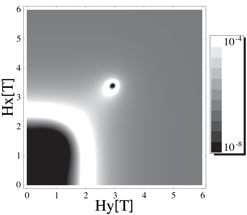
Figure 8 shows the cotunneling current as a function of the transverse magnetic field. Interestingly, the current is suppressed at the zeros of the tunnel splittings Δ1\Delta_{1} and Δ0\Delta_{0}, exactly as in the sequential tunneling regime.[17]

Refer to caption
Figure 8: Graph showing log10⁡I\log_{10}I versus the transverse magnetic field for Vb=VL−VR=4×10⁻³V_{b}=V_{L}-V_{R}=4\times 10^{-3}eV, Vg=0.01V_{g}=0.01eV and γ4,−4=1012\gamma_{4,-4}=10^{12}s-1. One can see that the current is suppressed at the zeros of the tunnel splittings Δ1\Delta_{1} and Δ0\Delta_{0}.

VI Conclusions

The main contribution of this paper is to show how the total Hamiltonian of a single-molecule magnet transistor can be mapped into the Kondo Hamiltonian by means of a Schrieffer-Wolff transformation. While the derivation of the effective Kondo Hamiltonian in other contexts, such as quantum dots and ordinary single (nonmagnetic) molecule coupled to leads is well-known, the case is different for SMM. The dominant Kondo effect is unusual for a SMM, since it involves a pseudospin of the molecule rather than its total spin. We show that if the total spin of the molecule is reduced (increased) for the charged states, the Kondo Hamiltonian exhibits an antiferromagnetic (ferromagnetic) coupling, leading to screening (anti-screening) of the total spin of the single-molecule magnet. In the case of antiferromagnetic coupling the renormalization leads to a Kondo effect, i.e. the conductance through the SMM exhibits a resonance at the Fermi energy. In the case of the ferromagnetic coupling the transverse exchange is renormalized to zero, in which case the Kondo resonance is absent. This result is in contrast to the case of the Kondo effect in lateral quantum dots exhibiting only antiferromagnetic exchange coupling, which is due to the fact that all the spin states are degenerate in the absence of anisotropies.[19] The standard Kondo screening of the molecule magnetization by itinerant electrons in the leads is a very weak effect in this context given the large spin of a SMM (its onset is therefore likely to occur only at exceedingly small temperatures, inaccessible to current experiments).

A careful derivation of the effective Kondo Hamiltonian shows that the strong dependence of this phenomenon on the amplitude and orientation of an external magnetic field. The strong uniaxial magnetic anisotropy of the SMM combined with the weaker in-plane anisotropy creates a pseudo spin 1/2 involving states with opposite magnetization orientation. A transverse magnetic field modulates the tunnel barrier between these states through a Berry phase interference effect. That, in turn, modulates periodically the Kondo effect in SMMs.

We have calculated the conductance of the single-molecule transistor in the presence of the Kondo effect by using the standard poor man’s scaling approach. We have show that in the case of antiferromagnetic Kondo exchange coupling by applying a transverse magnetic field to a single-molecule magnet with a large full- or half-integer spin S>1/2S>1/2 it is possible to topologically induce or quench the Kondo effect of the conductance of a current through the single-molecule magnet that is sufficiently well coupled to metallic leads. We have also shown how the zero points of the Berry phase oscillation become temperature dependent above the Kondo temperature and how they change direction within the plane (Fig. 4). The latter indicates that the parity of the Berry-phase oscillations [7, 8] changes from an integer spin S=4S=4 to a half-integer spin S=7/2S=7/2. We have also shown how this motion affects the temperature dependence of the conductance (see Fig. 6). Interestingly, the maximum value of the conductance encircles the zeros of the Berry phase oscillation, providing a mechanism for establishing the location of these zeros when the orientation of the molecule symmetry axis with respect to the metallic contacts is not known. We illustrate these features of the conductance of a SMM using as an example the new single-molecule magnet Ni4. In our view, due to its large ground state tunnel splitting this is currently the best SMM available for the experimental observation of the Berry-phase oscillations of the Kondo resonance.

Acknowledgments

The authors gratefully acknowledge useful discussions with George Christou, Enrique del Barco, Leonid Glazman, Chris Ramsey, and Peter Schmitteckert. E.R.M. acknowledges partial support through the NSF Grant No. CCF 0523603 and by the I2Lab at UCF. He also thanks the Max-Planck Institute for the Physics of Complex Systems for its hospitality. M.N.L. acknowledges partial support through the NSF Grant No. ECCS 0725514.

References

  • [1] A. Caneschi, J. Magn. Magn. Mater. 140-144, 379 (1995); J. R. Friedman, M. P. Sarachik, J. Tejada, and R. Ziolo, Phys. Rev. Lett. 76, 3830 (1996); L. Thomas, F. Lionti, R. Ballou, D. Gatteschi, R. Sessoli, and B. Barbara, Nature (London) 383, 145 (1996).
  • [2] E. del Barco, A. D. Kent, S. Hill, J. M. North, N. S. Dalal, E. M. Rumberger, D. N. Hendrickson, N. Chakov, G. Christou, J. Low Temp. Phys. 140, 119 (2005).
  • [3] C. Sangregorio, T. Ohm, C. Paulsen, R. Sessoli, and D. Gatteschi, Phys. Rev. Lett. 78, 4645 (1997).
  • [4] W. Wernsdorfer and R. Sessoli, Science 284, 133 (1999).
  • [5] E. Chudnovsky and L. Gunther, Phys. Rev. Lett. 60, 661 (1988); J. Tejada, E. M. Chudnovsky, E. del Barco, and J. M. Hernandez, Nanotechnology 12, 181 (2001); M. N. Leuenberger and D. Loss, Nature (London) 410, 789 (2001).
  • [6] W. Wernsdorfer, R. Sessoli, A. Caneschi, D. Gatteschi, and A. Cornia, Europhys. Lett. 50, 552 (2000); M. N. Leuenberger and D. Loss, Phys. Rev. B 61, 12200 (2000).
  • [7] D. Loss, D. P. DiVincenzo, and G. Grinstein, Phys. Rev. Lett. 69, 3232 (1992); J. von Delft and C. L. Henley, ibid. 69, 3236 (1992); A. Garg, Europhys. Lett. 22, 205 (1993).
  • [8] M. N. Leuenberger and D. Loss, Phys. Rev. B 63, 054414 (2001).
  • [9] H. B. Heersche, Z. de Groot, J. A. Folk, H. S. J. van der Zant, C. Romeike, M. R. Wegewijs, L. Zobbi, D. Barreca, E. Tondello, and A. Cornia Phys. Rev. Lett. 96, 206801 (2006).
  • [10] C. Romeike, M. R. Wegewijs, W. Hofstetter, and H. Schoeller, Phys. Rev. Lett. 96, 196601 (2006).
  • [11] M. R. Wegewijs, C. Romeike, H. Schoeller, and W. Hofstetter, New J. of Phys. 9, 344 (2007).
  • [12] M. N. Leuenberger and E. R. Mucciolo, Phys. Rev. Lett. 97, 126601 (2006).
  • [13] D. Goldhaber-Gordon, H. Shtrikman, D. Mahalu, D. Abusch-Madger, U. Meirav, and M. A. Kastner, Nature (London) 391, 156 (1998).
  • [14] A. Sieber, C. Boskovic, R. Bircher, O. Waldmann, S. T. Ochsenbein, G. Chaboussant, H.-U. Guedel, N. Kirchner, J. van Slageren, W. Wernsdorfer, A. Neels, H. Stoeckli-Evans, S. Janssen, F. Jurannyi, and H. Mutka, Inorg. Chem. 44, 4315 (2005).
  • [15] F. Elste, C. Timm, Phys. Rev. B 73, 235304 (2006); F. Elste, C. Timm, ibid. 73, 235305 (2006); F. Elste, C. Timm, ibid. 75, 195341 (2007); C. Timm, ibid. 76, 014421 (2007).
  • [16] J. R. Schrieffer and P. A. Wolff, Phys. Rev. 149, 491 (1966).
  • [17] G. González and M. N. Leuenberger, Phys. Rev. Lett. 98, 256804 (2007).
  • [18] A. C. Hewson, The Kondo Problem to Heavy Fermions (Cambridge University Press, 1997).
  • [19] L. I. Glazman and M. Pustilnik, in Nanophysics: Coherence and Transport, edited by H. Bouchiat et al. (Elsevier, 2005).
  • [20] The actual applied gate voltage is typically much larger than VgV_{g} due to screening and the setup geometry.
  • [21] R. Basler, A. Sieber, G. Chaboussant, H.-U. Guedel, N. E. Chakov, M. Soler, G. Christou, A. Desmedt, and R. Lechner, Inorg. Chem. 44, 649 (2005).
  • [22] Generalizations to include additional charge sectors are straightforward.
  • [23] The state with mq=0m_{q}=0 can be easily included in this description. However, since it typically requires a relatively high temperature or bias to be accessed, it will be neglected here.
  • [24] P. W. Anderson, J. Phys. C 3, 2436 (1970).
  • [25] S. R. White, Phys. Rev. Lett. 69, 2863 (1992).
  • [26] J. Appelbaum, Phys. Rev. 154, 633 (1967).
  • [27] J. Park, A. N. Pascupathy, J. I. Goldsmith, C. Chang, Y. Yaish, J. R. Petta, M. Rinkoski, J. P. Sethna, H. D. Abruna, P. L. McEuen, and D. C. Ralph, Nature (London) 417, 722 (2002).