跳到论文正文
W Papers独立论文阅读器 arXiv:0803.1212 论文正文 计算阅读时间 · 0%
引用这篇论文根据当前论文元数据生成,正式投稿前建议核对。


License: arXiv.org perpetual non-exclusive license
arXiv:0803.1212v3 [hep-th] 03 Apr 2008

An Exceptional Algebraic Origin
of the AdS/CFT Yangian Symmetry

Takuya Matsumoto ††thanks: m05044c@math.nagoya-u.ac.jp    and    Sanefumi Moriyama ††thanks: moriyama@math.nagoya-u.ac.jp Affiliation: Graduate School of Mathematics, Nagoya University, Affiliation: Nagoya 464-8602, Japan
March, 2008

In the 𝔰​𝔲​(2|2)\mathfrak{su}(2|2) spin chain motivated by the AdS/CFT correspondence, a novel symmetry extending the superalgebra 𝔰​𝔲​(2|2)\mathfrak{su}(2|2) into 𝔲⁡(2|2)\mathfrak{u}(2|2) was found. We pursue the origin of this symmetry in the exceptional superalgebra 𝔡⁡(2,1,ε)\mathfrak{d}(2,1;\varepsilon), which recovers 𝔰​𝔲​(2|2)\mathfrak{su}(2|2) when the parameter ε\varepsilon is taken to zero. Especially, we rederive the Yangian symmetries of the AdS/CFT spin chain using the exceptional superalgebra and find that the ε\varepsilon-correction corresponds to the novel symmetry. Also, we reproduce the non-canonical classical r-matrix of the AdS/CFT spin chain expressed with this symmetry from the canonical one of the exceptional algebra.

1 Introduction

Symmetry algebra always plays an important role in physics. The AdS/CFT correspondence is no exception, which relates the anomalous dimension of operators in 𝒩=4{\cal N}=4 super Yang-Mills theory with Hamiltonian of string states on the AdS5×S5{\rm AdS}_{5}\times{\rm S}^{5} spacetime. On the super Yang-Mills theory side, whose description is valid in the weak ’t Hooft coupling region λ=gYM2​N≪1\lambda=g_{\rm YM}^{2}N\ll 1, the perturbative dilatation operator was mapped to the Hamiltonian of an integrable spin chain model [1] where infinite conserved charges lead to solvability. On the string sigma model side, valid in the strong coupling region λ≫1\lambda\gg 1, flat connection which implies infinite symmetries was also constructed [2]. It was then expected that we can interpolate these two regions by integrability and solve the theory completely. See reviews [3] for a summary of current progress and a list of references.

This expectation was made more concrete in the subsequent analysis. The 𝒩=4{\mathcal{N}}=4 super Yang-Mills theory has a global symmetry of the Lie superalgebra 𝔭​𝔰​𝔲​(2,2|4)\mathfrak{psu}(2,2|4), which is broken down to two copies of 𝔰​𝔲​(2|2)\mathfrak{su}(2|2) algebra once we fix a vacuum. The spin chain model with this 𝔰​𝔲​(2|2)\mathfrak{su}(2|2) symmetry, which interpolates the two coupling regions, was constructed in [4]. To take care of the off-shell trace operators, the centrally extended 𝔰​𝔲​(2|2)\mathfrak{su}(2|2) superalgebra was considered, which contains not only the center of 𝔰​𝔲​(2|2)\mathfrak{su}(2|2), ℭ{\mathfrak{C}}, whose eigenvalue is the energy of the spin chain, but also two additional centers, 𝔓{\mathfrak{P}} and 𝔎{\mathfrak{K}}, whose eigenvalues correspond to the momentum and should vanish on the on-shell trace operators where the total momentum vanishes. In other words, this spin chain has the 𝔭​𝔰​𝔲​(2|2)⋉ℝ3\mathfrak{psu}(2|2)\ltimes\mathbb{R}^{3} symmetry. A remarkable property is that the S-matrix 𝒮{\mathcal{S}} on the fundamental representation is determined uniquely by the Lie algebraic symmetry up to an overall phase factor. It was also checked that this S-matrix satisfies the Yang-Baxter equation as the S-matrix of an integrable spin chain model is expected to.

In order to clarify the full symmetry structure, it is an important subject to study the universal R-matrix 𝒮=Π∘ℛ{\mathcal{S}}=\Pi\circ{\mathcal{R}} that does not depend on the representation. Here Π\Pi denotes the graded permutation operator. The first step to investigate the universal R-matrix is to study its classical limit ℛ12=1+ℏ​r12+𝒪⁡(ℏ2){\mathcal{R}}_{12}=1+\hbar r_{12}+{\mathcal{O}}(\hbar^{2}). It is known that a canonical form of the classical r-matrix

r12=𝒯12𝔤i⁡(u1−u2),\displaystyle r_{12}=\frac{\mathcal{T}_{12}^{\mathfrak{g}}}{i(u_{1}-u_{2})}~, (1.1)

is a solution to the classical Yang-Baxter equation, where 𝒯12𝔤\mathcal{T}_{12}^{\mathfrak{g}} is the two-site Casimir operator of the Lie algebra 𝔤\mathfrak{g} and uu is the spectral parameter. This fact is the starting point for the classification of solutions of the classical Yang-Baxter equation, as well as for the study of the symmetry structure [5, 6].

In the case of the AdS/CFT spin chain, however, the relevant Killing form of the centrally extended Lie superalgebra 𝔭​𝔰​𝔲​(2|2)⋉ℝ3\mathfrak{psu}(2|2)\ltimes{\mathbb{R}}^{3} is degenerate. Hence, the quadratic Casimir operator 𝒯𝔤\mathcal{T}^{\mathfrak{g}} commuting with all generators (and the corresponding two-site Casimir operator 𝒯12𝔤\mathcal{T}^{\mathfrak{g}}_{12}) does not exist in the strict sense. To cure the degeneracy of the Killing form, several different regularizations were proposed. The first one [4] is to consider the exceptional superalgebra 𝔡⁡(2,1,ε)\mathfrak{d}(2,1;\varepsilon) which recovers 𝔭​𝔰​𝔲​(2|2)⋉ℝ3\mathfrak{psu}(2|2)\ltimes{\mathbb{R}}^{3} when the parameter ε\varepsilon is taken to zero. In the exceptional algebra 𝔡⁡(2,1,ε)\mathfrak{d}(2,1;\varepsilon), the generators ℭ{\mathfrak{C}}, 𝔓{\mathfrak{P}} and 𝔎{\mathfrak{K}} are not central but form the usual 𝔰​𝔲​(2)\mathfrak{su}(2) algebra. The second one [7] is to couple the central charges to the 𝔰​𝔲​(2)\mathfrak{su}(2) outer automorphism, which has a similar origin as the above case. In [8], to find an expression for the classical r-matrix similar to (1.1), another regularization was adopted by introducing a new generator ℑ{\mathfrak{I}} which complements the original superalgebra 𝔰​𝔲​(2|2)\mathfrak{su}(2|2) into 𝔲⁡(2|2)\mathfrak{u}(2|2) and couples to the center of 𝔰​𝔲​(2|2)\mathfrak{su}(2|2). Subsequently, the corresponding coproduct and antipode of this new generator ℑ{\mathfrak{I}} at level-1 were proposed [9]

Δℑ^=ℑ^⊗1+1⊗ℑ^+ℏ2(𝔔α𝒰−1a⊗𝔖a+α𝔖a𝒰+1α⊗𝔔α)a,S(ℑ^)=−ℑ^+2ℏℭ,\displaystyle\Delta\widehat{\mathfrak{I}}=\widehat{\mathfrak{I}}\otimes 1+1\otimes\widehat{\mathfrak{I}}+\frac{\hbar}{2}\left({\mathfrak{Q}}^{\alpha}{}_{a}{\mathcal{U}}^{-1}\otimes{\mathfrak{S}}^{a}{}_{\alpha}+{\mathfrak{S}}^{a}{}_{\alpha}{\mathcal{U}}^{+1}\otimes{\mathfrak{Q}}^{\alpha}{}_{a}\right)~,\quad{\rm S}(\widehat{\mathfrak{I}})=-\widehat{\mathfrak{I}}+2\hbar{\mathfrak{C}}~, (1.2)

(with ℏ\hbar related to the ’t Hooft coupling λ\lambda by 1/ℏ=g=λ/4​π1/\hbar=g=\sqrt{\lambda}/{4\pi}) and found to be a symmetry of the fundamental S-matrix. However, it is still mysterious what the origin of this novel symmetry is.

Though the original proposal of the classical r-matrix is complicated, an elegant expression was found by [10]

r12\displaystyle r_{12} =𝒯12𝔭​𝔰​𝔲−𝒯𝔭​𝔰​𝔲​𝔇−1⊗𝔇−𝔇⊗𝒯𝔭​𝔰​𝔲​𝔇−1i⁡(u1−u2)\displaystyle=\frac{\mathcal{T}^{\mathfrak{psu}}_{12}-\mathcal{T}^{\mathfrak{psu}}{\mathfrak{D}}^{-1}\otimes{\mathfrak{D}}-{\mathfrak{D}}\otimes\mathcal{T}^{\mathfrak{psu}}{\mathfrak{D}}^{-1}}{i(u_{1}-u_{2})}
=𝒯12𝔭​𝔰​𝔲−(u1/u2)​𝒯𝔭​𝔰​𝔲​ℭ−1⊗ℭ−(u2/u1)​ℭ⊗𝒯𝔭​𝔰​𝔲​ℭ−1i⁡(u1−u2),\displaystyle=\frac{\mathcal{T}^{\mathfrak{psu}}_{12}-(u_{1}/u_{2})\mathcal{T}^{\mathfrak{psu}}{\mathfrak{C}}^{-1}\otimes{\mathfrak{C}}-(u_{2}/u_{1}){\mathfrak{C}}\otimes\mathcal{T}^{\mathfrak{psu}}{\mathfrak{C}}^{-1}}{i(u_{1}-u_{2})}~, (1.3)

where 𝒯𝔭​𝔰​𝔲\mathcal{T}^{\mathfrak{psu}} is the quadratic Casimir-like operator of 𝔭​𝔰​𝔲​(2|2)\mathfrak{psu}(2|2) and 𝒯12𝔭​𝔰​𝔲\mathcal{T}^{\mathfrak{psu}}_{12} is the corresponding two-site operator. In the above expression 𝔇{\mathfrak{D}} comes from the classical limit of the centers 𝔓{\mathfrak{P}} and 𝔎{\mathfrak{K}} and relates to ℭ{\mathfrak{C}} by 𝔇=2​u−1​ℭ{\mathfrak{D}}=2u^{-1}{\mathfrak{C}}. The Casimir-like operator 𝒯𝔭​𝔰​𝔲\mathcal{T}^{\mathfrak{psu}} takes the opposite sign on bosons and fermions

𝒯𝔭​𝔰​𝔲​|ϕa⟩=−14​|ϕa⟩,𝒯𝔭​𝔰​𝔲​|ψα⟩=+14​|ψα⟩,\displaystyle\mathcal{T}^{\mathfrak{psu}}|\phi^{a}\rangle=-\frac{1}{4}|\phi^{a}\rangle~,\quad\mathcal{T}^{\mathfrak{psu}}|\psi^{\alpha}\rangle=+\frac{1}{4}|\psi^{\alpha}\rangle~, (1.4)

and serves the same role as ℑ{\mathfrak{I}}. Interestingly, it was further noted that the eigenvalue of the new generator ℑ{\mathfrak{I}} and the composite operator 𝒯𝔭​𝔰​𝔲​ℭ−1\mathcal{T}^{\mathfrak{psu}}{\mathfrak{C}}^{-1} coincides and that both the composite operator 𝒯𝔭​𝔰​𝔲​ℭ−1\mathcal{T}^{\mathfrak{psu}}{\mathfrak{C}}^{-1} and the Cartan generator of the 𝔰​𝔲​(2)\mathfrak{su}(2) outer automorphism 2𝔅=𝔅11−𝔅222{\mathfrak{B}}={\mathfrak{B}}^{1}{}_{1}-{\mathfrak{B}}^{2}{}_{2} satisfy similar commutation relations.

The above classical r-matrix (1.3) implies a beautiful Lie bialgebraic structure. Especially, the classical cobrackets of all the generators, including the new one ℑ{\mathfrak{I}}, were constructed. This analysis indicates, among others, the Yangian symmetries of the generator ℑ{\mathfrak{I}} of all levels. However, unfortunately, aside from the level-1 Yangian symmetry (1.2), we cannot show that they are exact quantum symmetries of the fundamental S-matrix. We believe that this unsatisfactory fact stems from the non-canonical form of the classical r-matrix (1.3), or in other words, the degeneracy of the Killing form of 𝔭​𝔰​𝔲​(2|2)⋉ℝ3\mathfrak{psu}(2|2)\ltimes{\mathbb{R}}^{3}.

In this paper we would like to pursue the origin of this novel generator in the exceptional superalgebra 𝔡⁡(2,1,ε)\mathfrak{d}(2,1;\varepsilon) and interpret the symmetry ℑ{\mathfrak{I}} as the ε\varepsilon-correction of the generators ℭ{\mathfrak{C}}, 𝔓{\mathfrak{P}} and 𝔎{\mathfrak{K}}. We first investigate the Yangian coproducts of ℭ{\mathfrak{C}}, 𝔓{\mathfrak{P}} and 𝔎{\mathfrak{K}} in the exceptional superalgebra 𝔡⁡(2,1,ε)\mathfrak{d}(2,1;\varepsilon) and show that the non-trivial coproduct of ℑ{\mathfrak{I}} (1.2) coincides with the ε\varepsilon-correction of the coproduct of ℭ{\mathfrak{C}}. Secondly, we shall reproduce the classical r-matrix (1.3) by taking the ε→0\varepsilon\to 0 limit in the canonical classical r-matrix of the exceptional superalgebra 𝔡⁡(2,1,ε)\mathfrak{d}(2,1;\varepsilon):

r12=𝒯12𝔡i⁡(u1−u2)|ε→0,\displaystyle r_{12}=\frac{\mathcal{T}^{\mathfrak{d}}_{12}}{i(u_{1}-u_{2})}\Big|_{\varepsilon\to 0}~, (1.5)

where T12𝔡T^{\mathfrak{d}}_{12} is the two-site quadratic Casimir operator of 𝔡⁡(2,1,ε)\mathfrak{d}(2,1;\varepsilon). Since the generators ℭ{\mathfrak{C}}, 𝔓{\mathfrak{P}} and 𝔎{\mathfrak{K}} in 𝔡⁡(2,1,ε)\mathfrak{d}(2,1;\varepsilon) are not central, the action on bosons and fermions is slightly different. As we shall see later, this is the origin of ℑ{\mathfrak{I}} in the exceptional algebra 𝔡⁡(2,1,ε)\mathfrak{d}(2,1;\varepsilon).

In the next section we first review the exceptional superalgebra 𝔡⁡(2,1,ε)\mathfrak{d}(2,1;\varepsilon) and the 𝔰​𝔲​(2|2)\mathfrak{su}(2|2) spin chain model. In section 3, We proceed to studying the Yangian coproducts of all the 𝔭​𝔰​𝔲​(2|2)⋉ℝ3\mathfrak{psu}(2|2)\ltimes{\mathbb{R}}^{3} generators from the superalgebra 𝔡⁡(2,1,ε)\mathfrak{d}(2,1;\varepsilon) and find that the non-trivial coproduct of the symmetry ℑ{\mathfrak{I}} coincides with the ε\varepsilon-correction of that of ℭ{\mathfrak{C}}. Then we reproduce the non-canonical AdS/CFT classical r-matrix from the canonical one of 𝔡⁡(2,1,ε)\mathfrak{d}(2,1;\varepsilon) in section 4. Finally in section 5, we conclude with some discussions.

2 Review of the exceptional Lie superalgebra

In this section we would like to review the exceptional Lie superalgebra 𝔡⁡(2,1,ε)\mathfrak{d}(2,1;\varepsilon), the limit which recovers the symmetry 𝔭​𝔰​𝔲​(2|2)⋉ℝ3\mathfrak{psu}(2|2)\ltimes{\mathbb{R}}^{3} and the AdS/CFT spin chain with this symmetry [4].

2.1 Exceptional Superalgebra 𝔡⁡(2,1,ε)\mathfrak{d}(2,1;\varepsilon)

The exceptional Lie superalgebra 𝔡⁡(2,1,ε)\mathfrak{d}(2,1;\varepsilon) is given by three orthogonal sets of 𝔰​𝔲​(2)\mathfrak{su}(2) triplet bosonic generators ℜab{\mathfrak{R}}^{a}{}_{b}, 𝔏αβ{\mathfrak{L}}^{\alpha}{}_{\beta}, ℭ𝔞𝔟{\mathfrak{C}}^{\mathfrak{a}}{}_{\mathfrak{b}} and an octet of fermionic generators 𝔉a​α​𝔞{\mathfrak{F}}^{a\alpha\mathfrak{a}}. The non-trivial commutation relations between the 𝔰​𝔲​(2)\mathfrak{su}(2) bosonic generators are given by

[ℜa,bℜc]d=δbcℜa−dδdaℜc,b[𝔏α,β𝔏γ]δ=δβγ𝔏α−δδδα𝔏γ,β[ℭ𝔞,𝔟ℭ𝔠]𝔡=δ𝔟𝔠ℭ𝔞−𝔡δ𝔡𝔞ℭ𝔠,𝔟\displaystyle[{\mathfrak{R}}^{a}{}_{b},{\mathfrak{R}}^{c}{}_{d}]=\delta^{c}_{b}{\mathfrak{R}}^{a}{}_{d}-\delta^{a}_{d}{\mathfrak{R}}^{c}{}_{b}~,\quad[{\mathfrak{L}}^{\alpha}{}_{\beta},{\mathfrak{L}}^{\gamma}{}_{\delta}]=\delta^{\gamma}_{\beta}{\mathfrak{L}}^{\alpha}{}_{\delta}-\delta^{\alpha}_{\delta}{\mathfrak{L}}^{\gamma}{}_{\beta}~,\quad[{\mathfrak{C}}^{\mathfrak{a}}{}_{\mathfrak{b}},{\mathfrak{C}}^{\mathfrak{c}}{}_{\mathfrak{d}}]=\delta^{\mathfrak{c}}_{\mathfrak{b}}{\mathfrak{C}}^{\mathfrak{a}}{}_{\mathfrak{d}}-\delta^{\mathfrak{a}}_{\mathfrak{d}}{\mathfrak{C}}^{\mathfrak{c}}{}_{\mathfrak{b}}~, (2.1)

while the fermionic generators transform in the fundamental representation of each 𝔰​𝔲​(2)\mathfrak{su}(2) as

[ℜa,b𝔉c​γ​𝔠]=δbc𝔉a​γ​𝔠−12δba𝔉c​γ​𝔠,[𝔏α,β𝔉c​γ​𝔠]=δβγ𝔉c​α​𝔠−12δβα𝔉c​γ​𝔠,[ℭ𝔞,𝔟𝔉c​γ​𝔠]=δ𝔟𝔠𝔉c​γ​𝔞−12δ𝔟𝔞𝔉c​γ​𝔠.\displaystyle[{\mathfrak{R}}^{a}{}_{b},{\mathfrak{F}}^{c\gamma\mathfrak{c}}]=\delta^{c}_{b}{\mathfrak{F}}^{a\gamma\mathfrak{c}}\!-\!\frac{1}{2}\delta^{a}_{b}{\mathfrak{F}}^{c\gamma\mathfrak{c}},\quad[{\mathfrak{L}}^{\alpha}{}_{\beta},{\mathfrak{F}}^{c\gamma\mathfrak{c}}]=\delta^{\gamma}_{\beta}{\mathfrak{F}}^{c\alpha\mathfrak{c}}\!-\!\frac{1}{2}\delta^{\alpha}_{\beta}{\mathfrak{F}}^{c\gamma\mathfrak{c}},\quad[{\mathfrak{C}}^{\mathfrak{a}}{}_{\mathfrak{b}},{\mathfrak{F}}^{c\gamma\mathfrak{c}}]=\delta^{\mathfrak{c}}_{\mathfrak{b}}{\mathfrak{F}}^{c\gamma\mathfrak{a}}\!-\!\frac{1}{2}\delta^{\mathfrak{a}}_{\mathfrak{b}}{\mathfrak{F}}^{c\gamma\mathfrak{c}}. (2.2)

Also, the anti-commutation relation between the fermionic generators is

{𝔉a​α​𝔞,𝔉b​β​𝔟}=αϵa​kϵα​βϵ𝔞​𝔟ℜb+kβϵa​bϵα​κϵ𝔞​𝔟𝔏β+κγϵa​bϵα​βϵ𝔞​𝔨ℭ𝔟,𝔨\displaystyle\{{\mathfrak{F}}^{a\alpha\mathfrak{a}},{\mathfrak{F}}^{b\beta\mathfrak{b}}\}=\alpha\epsilon^{ak}\epsilon^{\alpha\beta}\epsilon^{\mathfrak{a}\mathfrak{b}}{\mathfrak{R}}^{b}{}_{k}+\beta\epsilon^{ab}\epsilon^{\alpha\kappa}\epsilon^{\mathfrak{a}\mathfrak{b}}{\mathfrak{L}}^{\beta}{}_{\kappa}+\gamma\epsilon^{ab}\epsilon^{\alpha\beta}\epsilon^{\mathfrak{a}\mathfrak{k}}{\mathfrak{C}}^{\mathfrak{b}}{}_{\mathfrak{k}}~, (2.3)

where the constants α\alpha, β\beta, γ\gamma have to satisfy α+β+γ=0\alpha+\beta+\gamma=0 due to the Jacobi identity. Since the overall rescaling does not change the algebraic structure, the only one parameter which characterizes 𝔡⁡(2,1,ε)\mathfrak{d}(2,1;\varepsilon) is ε=−γ/α\varepsilon=-\gamma/\alpha. The Killing form of this algebra is non-degenerate, and therefore, this algebra has a well-defined quadratic Casimir operator,

𝒯𝔡=12(−αℜaℜbb−aβ𝔏α𝔏ββ−αγℭ𝔞ℭ𝔟𝔟−𝔞ϵa​bϵα​βϵ𝔞​𝔟𝔉a​α​𝔞𝔉b​β​𝔟).\displaystyle\mathcal{T}^{\mathfrak{d}}=\frac{1}{2}\Bigl(-\alpha\mathfrak{R}^{a}{}_{b}\mathfrak{R}^{b}{}_{a}-\beta\mathfrak{L}^{\alpha}{}_{\beta}\mathfrak{L}^{\beta}{}_{\alpha}-\gamma\mathfrak{C}^{\mathfrak{a}}{}_{\mathfrak{b}}\mathfrak{C}^{\mathfrak{b}}{}_{\mathfrak{a}}-\epsilon_{ab}\epsilon_{\alpha\beta}\epsilon_{\mathfrak{a}\mathfrak{b}}{\mathfrak{F}}^{a\alpha\mathfrak{a}}{\mathfrak{F}}^{b\beta\mathfrak{b}}\Bigr)~. (2.4)

To reproduce the centrally extended superalgebra 𝔭​𝔰​𝔲​(2|2)⋉ℝ3\mathfrak{psu}(2|2)\ltimes{\mathbb{R}}^{3}, let us choose

α=−1,β=1−ε,γ=ε,\displaystyle\alpha=-1~,\quad\beta=1-\varepsilon~,\quad\gamma=\varepsilon~, (2.5)

and take the limit ε→0\varepsilon\to 0. To avoid the singular behavior and match the convention with the usual one used in 𝔭​𝔰​𝔲​(2|2)⋉ℝ3\mathfrak{psu}(2|2)\ltimes{\mathbb{R}}^{3}, let us further rewrite the last bosonic 𝔰​𝔲​(2)\mathfrak{su}(2) generator ℭ𝔞𝔟{\mathfrak{C}}^{\mathfrak{a}}{}_{\mathfrak{b}} and the fermionic generator 𝔉a​α​𝔞{\mathfrak{F}}^{a\alpha\mathfrak{a}} as

(ℭ)=𝔞𝔟1ε(ℭ𝔓−𝔎−ℭ),(𝔉a​α)=𝔞(ϵa​k𝔔αkϵα​κ𝔖aκ).\displaystyle({\mathfrak{C}}){}^{\mathfrak{a}}{}_{\mathfrak{b}}=\frac{1}{\varepsilon}\begin{pmatrix}{\mathfrak{C}}&{\mathfrak{P}}\\ -{\mathfrak{K}}&-{\mathfrak{C}}\end{pmatrix}~,\quad({\mathfrak{F}}^{a\alpha}){}^{\mathfrak{a}}=\begin{pmatrix}\epsilon^{ak}{\mathfrak{Q}}^{\alpha}{}_{k}\\ \epsilon^{\alpha\kappa}{\mathfrak{S}}^{a}{}_{\kappa}\end{pmatrix}~. (2.6)

In the new convention, the anti-commutation relations between the fermionic generators become

{𝔔α,a𝔔β}b\displaystyle\{{\mathfrak{Q}}^{\alpha}{}_{a},{\mathfrak{Q}}^{\beta}{}_{b}\} =ϵα​β​ϵa​b​𝔓,\displaystyle=\epsilon^{\alpha\beta}\epsilon_{ab}{\mathfrak{P}}~,
{𝔖a,α𝔖b}β\displaystyle\{{\mathfrak{S}}^{a}{}_{\alpha},{\mathfrak{S}}^{b}{}_{\beta}\} =ϵa​b​ϵα​β​𝔎,\displaystyle=\epsilon^{ab}\epsilon_{\alpha\beta}{\mathfrak{K}}~,
{𝔔α,a𝔖b}β\displaystyle\{{\mathfrak{Q}}^{\alpha}{}_{a},{\mathfrak{S}}^{b}{}_{\beta}\} =δβαℜb+a(1−ε)δab𝔏α+βδβαδabℭ,\displaystyle=\delta^{\alpha}_{\beta}{\mathfrak{R}}^{b}{}_{a}+(1-\varepsilon)\delta^{b}_{a}{\mathfrak{L}}^{\alpha}{}_{\beta}+\delta^{\alpha}_{\beta}\delta^{b}_{a}{\mathfrak{C}}~, (2.7)

while the commutation relations involving the last bosonic 𝔰​𝔲​(2)\mathfrak{su}(2) generators are

[ℭ,𝔓]=ε​𝔓,[ℭ,𝔎]=−ε​𝔎,[𝔓,𝔎]=−2​ε​ℭ,\displaystyle[{\mathfrak{C}},{\mathfrak{P}}]=\varepsilon{\mathfrak{P}}~,\quad[{\mathfrak{C}},{\mathfrak{K}}]=-\varepsilon{\mathfrak{K}}~,\quad[{\mathfrak{P}},{\mathfrak{K}}]=-2\varepsilon{\mathfrak{C}}~,
[ℭ,𝔔α]a=+(ε/2)𝔔α,a[𝔓,𝔔α]a=0,[𝔎,𝔔α]a=εϵα​βϵa​b𝔖b,β\displaystyle[{\mathfrak{C}},{\mathfrak{Q}}^{\alpha}{}_{a}]=+(\varepsilon/2){\mathfrak{Q}}^{\alpha}{}_{a}~,\quad[{\mathfrak{P}},{\mathfrak{Q}}^{\alpha}{}_{a}]=0~,\quad[{\mathfrak{K}},{\mathfrak{Q}}^{\alpha}{}_{a}]=\varepsilon\epsilon^{\alpha\beta}\epsilon_{ab}{\mathfrak{S}}^{b}{}_{\beta}~,
[ℭ,𝔖a]α=−(ε/2)𝔖a,α[𝔓,𝔖a]α=−εϵa​bϵα​β𝔔β,b[𝔎,𝔖a]α=0.\displaystyle[{\mathfrak{C}},{\mathfrak{S}}^{a}{}_{\alpha}]=-(\varepsilon/2){\mathfrak{S}}^{a}{}_{\alpha}~,\quad[{\mathfrak{P}},{\mathfrak{S}}^{a}{}_{\alpha}]=-\varepsilon\epsilon^{ab}\epsilon_{\alpha\beta}{\mathfrak{Q}}^{\beta}{}_{b}~,\quad[{\mathfrak{K}},{\mathfrak{S}}^{a}{}_{\alpha}]=0~. (2.8)

The rest commutation relations involving the other two 𝔰​𝔲​(2)\mathfrak{su}(2) generators ℜab{\mathfrak{R}}^{a}{}_{b} and 𝔏αβ{\mathfrak{L}}^{\alpha}{}_{\beta} do not contain the parameter ε\varepsilon. These commutation relations are easily identified with those of 𝔭​𝔰​𝔲​(2|2)⋉ℝ3\mathfrak{psu}(2|2)\ltimes{\mathbb{R}}^{3} in the limit ε→0\varepsilon\to 0. Note that, among others, ℭ{\mathfrak{C}}, 𝔓{\mathfrak{P}} and 𝔎{\mathfrak{K}} become central in this limit.

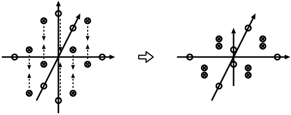
The root lattice should be helpful in understanding the ε→0\varepsilon\to 0 limit intuitively. (See Fig. 1.) As we will see in subsection 4.2, the additional dimension of the 𝔡⁡(2,1,ε)\mathfrak{d}(2,1;\varepsilon) root lattice plays an important role in constructing the representation of 𝔡⁡(2,1,ε)\mathfrak{d}(2,1;\varepsilon). In the next subsection let us recapitulate the representation of 𝔭​𝔰​𝔲​(2|2)⋉ℝ3\mathfrak{psu}(2|2)\ltimes{\mathbb{R}}^{3} first.

Refer to caption
R R 1 2 R 2 1 L L 1 2 L 2 1 C P K Q 1 2 S 1 2 Q 2 2 S 1 1 Q 1 1 S 2 2 Q 2 1 S 2 1 C R L → ε 0
Figure 1: Root lattice of 𝔡⁡(2,1,ε)\mathfrak{d}(2,1;\varepsilon) and the limit to reproduce 𝔭​𝔰​𝔲​(2|2)⋉ℝ3\mathfrak{psu}(2|2)\ltimes{\mathbb{R}}^{3}. Here we have defined ℜ=(ℜ1−1ℜ2)2/2{\mathfrak{R}}=({\mathfrak{R}}^{1}{}_{1}-{\mathfrak{R}}^{2}{}_{2})/2 and 𝔏=(𝔏1−1𝔏2)2/2{\mathfrak{L}}=({\mathfrak{L}}^{1}{}_{1}-{\mathfrak{L}}^{2}{}_{2})/2.

2.2 Fundamental representation of 𝔭​𝔰​𝔲​(2|2)⋉ℝ3\mathfrak{psu}(2|2)\ltimes{\mathbb{R}}^{3}

The algebra 𝔭​𝔰​𝔲​(2|2)⋉ℝ3\mathfrak{psu}(2|2)\ltimes{\mathbb{R}}^{3} has a 𝟐|𝟐\boldsymbol{2}|\boldsymbol{2}-dimensional representation, which is called the fundamental representation. The states in the representation space are labeled by two bosons |ϕa⟩|\phi^{a}\rangle and two fermions |ψα⟩|\psi^{\alpha}\rangle.

This representation has a physical meaning in the 𝔰​𝔲​(2|2)\mathfrak{su}(2|2) spin chain model motivated by super Yang-Mills theory. In the model, the vacuum state is identified with the infinitely long trace operator

|0⟩=|𝒵𝒵⋯𝒵⟩⇔Tr(𝒵𝒵⋯𝒵),\displaystyle|0\rangle=|{\mathcal{Z}}{\mathcal{Z}}\cdots{\mathcal{Z}}\rangle\quad\Leftrightarrow\quad{\rm Tr}({\mathcal{Z}}{\mathcal{Z}}\cdots{\mathcal{Z}})~, (2.9)

where 𝒵{\mathcal{Z}} corresponds to one of the complex scalar fields in super Yang-Mills theory. This identification of the vacuum state breaks the original global 𝔭​𝔰​𝔲​(2,2|4)\mathfrak{psu}(2,2|4) symmetry into two copies of the 𝔰​𝔲​(2|2)\mathfrak{su}(2|2) symmetry. Hence, the excitation of the original super Yang-Mills theory is expressed by two excitations in each 𝔰​𝔲​(2|2)\mathfrak{su}(2|2) spin chain. The excitation χ∈{ϕ1,ϕ2|ψ1,ψ2}\chi\in\{\phi^{1},\phi^{2}|\psi^{1},\psi^{2}\} in the 𝔰​𝔲​(2|2)\mathfrak{su}(2|2) spin chain form the fundamental representation of 𝔰​𝔲​(2|2)\mathfrak{su}(2|2). We shall consider the KK-magnon asymptotic state where the excitations are well-separated:

|χ1χ2′⋯χK′′⟩=∑n1≪n2≪⋯≪nKei​p1​n1ei​p2​n2⋯ei​pK​nK|𝒵⋯𝒵χ1𝒵⋯𝒵χ2′𝒵⋯𝒵χK′′𝒵⋯𝒵⟩,\displaystyle|\chi_{1}\chi^{\prime}_{2}\cdots\chi^{\prime\prime}_{K}\rangle=\sum_{n_{1}\ll n_{2}\ll\cdots\ll n_{K}}e^{ip_{1}n_{1}}e^{ip_{2}n_{2}}\cdots e^{ip_{K}n_{K}}|{\mathcal{Z}}\cdots{\mathcal{Z}}\chi_{1}{\mathcal{Z}}\cdots{\mathcal{Z}}\chi^{\prime}_{2}{\mathcal{Z}}\cdots{\mathcal{Z}}\chi^{\prime\prime}_{K}{\mathcal{Z}}\cdots{\mathcal{Z}}\rangle~, (2.10)

with nkn_{k} denoting the site of the kk-th excitation χk\chi_{k}. Here, the excitation χk\chi_{k} carries the momentum pkp_{k} on the spin chain.

Refer to caption
R L | ϕ 1 ⟩ | ϕ 2 ⟩ | ψ 1 ⟩ | ψ 2 ⟩
Figure 2: Weight lattice of the fundamental representation of 𝔭​𝔰​𝔲​(2|2)\mathfrak{psu}(2|2).

The two sets of 𝔰​𝔲​(2)\mathfrak{su}(2) bosonic generators ℜab{\mathfrak{R}}^{a}{}_{b} and 𝔏αβ{\mathfrak{L}}^{\alpha}{}_{\beta} act kinematically on the states:

ℜa|bϕkc⟩=δbc|ϕka⟩−12δba|ϕkc⟩,𝔏α|βψkγ⟩=δβγ|ψkα⟩−12δβα|ψkγ⟩.\displaystyle{\mathfrak{R}}^{a}{}_{b}|\phi^{c}_{k}\rangle=\delta^{c}_{b}|\phi^{a}_{k}\rangle-\dfrac{1}{2}\delta^{a}_{b}|\phi^{c}_{k}\rangle~,\quad{\mathfrak{L}}^{\alpha}{}_{\beta}|\psi^{\gamma}_{k}\rangle=\delta^{\gamma}_{\beta}|\psi^{\alpha}_{k}\rangle-\dfrac{1}{2}\delta^{\alpha}_{\beta}|\psi^{\gamma}_{k}\rangle~. (2.11)

Let us postulate the generic action of the fermionic generators 𝔔αa{\mathfrak{Q}}^{\alpha}{}_{a} and 𝔖aα{\mathfrak{S}}^{a}{}_{\alpha} as

𝔔α|aϕkb⟩=akδab|𝒵+1/2ψkα⟩,𝔔α|aψkβ⟩=bkϵα​βϵa​b|𝒵+1/2ϕkb⟩,\displaystyle{{\mathfrak{Q}}}^{\alpha}{}_{a}|\phi^{b}_{k}\rangle=a_{k}{\,}\delta^{b}_{a}|{\mathcal{Z}}^{+1/2}\psi^{\alpha}_{k}\rangle~,\quad{{\mathfrak{Q}}}^{\alpha}{}_{a}|\psi^{\beta}_{k}\rangle=b_{k}{\,}\epsilon^{\alpha\beta}\epsilon_{ab}|{\mathcal{Z}}^{+1/2}\phi^{b}_{k}\rangle~,
𝔖a|αϕkb⟩=ckϵa​bϵα​β|𝒵−1/2ψkβ⟩,𝔖a|αψkβ⟩=dkδαβ|𝒵−1/2ϕka⟩.\displaystyle{{\mathfrak{S}}}^{a}{}_{\alpha}|\phi^{b}_{k}\rangle=c_{k}{\,}\epsilon^{ab}\epsilon_{\alpha\beta}|{\mathcal{Z}}^{-1/2}\psi^{\beta}_{k}\rangle~,\quad{{\mathfrak{S}}}^{a}{}_{\alpha}|\psi^{\beta}_{k}\rangle=d_{k}{\,}\delta^{\beta}_{\alpha}|{\mathcal{Z}}^{-1/2}\phi^{a}_{k}\rangle~. (2.12)

(See Fig. 2.) Here 𝒵±1(/2){\mathcal{Z}}^{\pm 1(/2)} stands for insertion or removal of (half of) the 𝒵{\mathcal{Z}} field. This is important when we consider the action on the multi-magnon state. If we stick to the convention of placing the extra 𝒵{\mathcal{Z}} fields on the most left, a braiding factor Uk=ei​pk/2U_{k}=e^{ip_{k}/2} will emerge in moving the 𝒵{\mathcal{Z}} field to the left as in |χk​𝒵n⟩=Uk2​n​|𝒵n​χk⟩|\chi_{k}{\mathcal{Z}}^{n}\rangle=U_{k}^{2n}|{\mathcal{Z}}^{n}\chi_{k}\rangle. This effect can alternatively be interpreted as the inclusion of a braiding factor Uk=ei​pk/2U_{k}=e^{ip_{k}/2} in the tensor product such as coproducts and two-site Casimir operators [11]. The power of the 𝒵{\mathcal{Z}} field nn, which depends on the generators, is called grading and corresponds to the eigenvalues of ℭ{\mathfrak{C}} in the adjoint representation (2.8) (in the unit of ε\varepsilon).

The consistency condition with the algebra, especially (2.7) in the limit ε→0\varepsilon\to 0, requires the coefficients aka_{k}, bkb_{k}, ckc_{k} and dkd_{k} to satisfy the relation

ak​dk−bk​ck=1,\displaystyle a_{k}d_{k}-b_{k}c_{k}=1~, (2.13)

as well as determines the action of centers ℭ{\mathfrak{C}}, 𝔓{\mathfrak{P}} and 𝔎{\mathfrak{K}}

ℭ⁡|χk⟩=12​(ak​dk+bk​ck)​|χk⟩,𝔓⁡|χk⟩=ak​bk​|𝒵+1​χk⟩,𝔎⁡|χk⟩=ck​dk​|𝒵−1​χk⟩,\displaystyle{\mathfrak{C}}|\chi_{k}\rangle=\dfrac{1}{2}(a_{k}d_{k}+b_{k}c_{k})|\chi_{k}\rangle~,\quad{\mathfrak{P}}|\chi_{k}\rangle=a_{k}b_{k}|{\mathcal{Z}}^{+1}\chi_{k}\rangle~,\quad{\mathfrak{K}}|\chi_{k}\rangle=c_{k}d_{k}|{\mathcal{Z}}^{-1}\chi_{k}\rangle~, (2.14)

where χk\chi_{k} is an arbitrary kk-th excitation. The coefficients aka_{k}, bkb_{k}, ckc_{k} and dkd_{k} are expressed by parameters xk±x^{\pm}_{k}, γk\gamma_{k} and a constant α\alpha:

ak=g​γk,bk=g​αγk​(1−xk+xk−),ck=g​i​γkα​xk+,dk=g​xk+i​γk​(1−xk−xk+),\displaystyle a_{k}=\sqrt{g}\gamma_{k}~,\quad b_{k}=\sqrt{g}\frac{\alpha}{\gamma_{k}}\left(1-\frac{x^{+}_{k}}{x^{-}_{k}}\right)~,\quad c_{k}=\sqrt{g}\frac{i\gamma_{k}}{\alpha x^{+}_{k}}~,\quad d_{k}=\sqrt{g}\frac{x^{+}_{k}}{i\gamma_{k}}\left(1-\frac{x^{-}_{k}}{x^{+}_{k}}\right)~, (2.15)

where the parameters xk±x^{\pm}_{k} relate to the momentum of the kk-th excitation by

xk+xk−=ei​pk(=Uk2),\displaystyle\frac{x^{+}_{k}}{x^{-}_{k}}=e^{ip_{k}}(=U_{k}^{2})~, (2.16)

and obey the constraint

xk++1xk+−xk−−1xk−=ig.\displaystyle x^{+}_{k}+\frac{1}{x^{+}_{k}}-x^{-}_{k}-\frac{1}{x^{-}_{k}}=\frac{i}{g}~. (2.17)

Note that we have required the extra central charges 𝔓{\mathfrak{P}} and 𝔎{\mathfrak{K}} to vanish on the on-shell states where the total momentum vanishes. This is why the parameter α\alpha has to be a constant independent of the excitations.

The constraint (2.17) can be solved explicitly [12]

xk±=xk​(1−1[2​g​(xk−xk−1)]2±i2​g​(xk−xk−1)).\displaystyle x^{\pm}_{k}=x_{k}\biggl(\sqrt{1-\frac{1}{[2g(x_{k}-x_{k}^{-1})]^{2}}}\pm\frac{i}{2g(x_{k}-x_{k}^{-1})}\biggr)~. (2.18)

In the classical limit g→∞g\to\infty, the coefficients aka_{k}, bkb_{k}, ckc_{k} and dkd_{k} can be expressed as [13]

ak=g​γk,bk=αi​g​γk​1xk−xk−1,ck=i​g​γkα​xk−1,dk=1g​γk​xkxk−xk−1.\displaystyle a_{k}=\sqrt{g}\gamma_{k}~,\quad b_{k}=\frac{\alpha}{i\sqrt{g}\gamma_{k}}\frac{1}{x_{k}-x_{k}^{-1}}~,\quad c_{k}=\frac{i\sqrt{g}\gamma_{k}}{\alpha}x_{k}^{-1}~,\quad d_{k}=\frac{1}{\sqrt{g}\gamma_{k}}\frac{x_{k}}{x_{k}-x_{k}^{-1}}~. (2.19)

To keep all the variables finite in the classical limit, we assume that γk\gamma_{k} scales as 1/g1/\sqrt{g}. Note that in the classical limit, the braiding factor reduces to Uk=1U_{k}=1.

3 Yangian coproducts from 𝔡⁡(2,1,ε)\mathfrak{d}(2,1;\varepsilon)

After reviewing the superalgebra 𝔡⁡(2,1,ε)\mathfrak{d}(2,1;\varepsilon) and the limit leading to the symmetry 𝔭​𝔰​𝔲​(2|2)⋉ℝ3\mathfrak{psu}(2|2)\ltimes{\mathbb{R}}^{3}, let us turn to the subject of this paper. We shall reproduce the coproducts of the generators in 𝔭​𝔰​𝔲​(2|2)⋉ℝ3\mathfrak{psu}(2|2)\ltimes{\mathbb{R}}^{3} from those in 𝔡⁡(2,1,ε)\mathfrak{d}(2,1;\varepsilon). In the derivation, we will see the first sign that the novel generator ℑ{\mathfrak{I}} [8, 9, 10] can be interpreted as the ε\varepsilon-correction of the last 𝔰​𝔲​(2)\mathfrak{su}(2) generators ℭ𝔞𝔟{\mathfrak{C}}^{\mathfrak{a}}{}_{\mathfrak{b}}.

A model is solvable if it has an equal number of conserved charges and degrees of freedom. For a solvable field-theoretical model with infinite degrees of freedom, we expect infinite conserved charges. In the field-theoretical model the scattering process between incoming and outgoing states is described by the S-matrix. For the solvable model, it is often the case that multi-body S-matrix factorizes into the product of two-body S-matrix. To see the symmetry of the S-matrix, we have to specify how the symmetries 𝔍A{\mathfrak{J}}^{A} act on two-body states, which can be non-local. The mathematical words for this action is called coproduct Δ​𝔍A\Delta{\mathfrak{J}}^{A}. The R-matrix ℛ=Π∘𝒮{\mathcal{R}}=\Pi\circ{\mathcal{S}} of the rational type has a symmetry called the Yangian algebra [Δ​𝔍^A,𝒮]=0[\Delta\widehat{\mathfrak{J}}^{A},{\mathcal{S}}]=0, besides the Lie algebraic symmetries [Δ​𝔍A,𝒮]=0[\Delta{\mathfrak{J}}^{A},{\mathcal{S}}]=0. In general, the Yangian algebra Y⁡(𝔤)Y(\mathfrak{g}), associated with Lie algebra 𝔤\mathfrak{g}, is a kind of the universal enveloping algebra U⁡(𝔤⁡[u,u−1])U(\mathfrak{g}[u,u^{-1}]) of the loop algebra 𝔤⁡[u,u−1]\mathfrak{g}[u,u^{-1}].

In [14], the level-1 Yangian symmetry 𝔍^A=i​u​𝔍A\widehat{\mathfrak{J}}^{A}=iu{\mathfrak{J}}^{A} (on the evaluation representation) associated with 𝔭​𝔰​𝔲​(2|2)⋉ℝ3\mathfrak{psu}(2|2)\ltimes{\mathbb{R}}^{3} is obtained from the standard formula [6]

Δ​𝔍^A=𝔍^A⊗1+𝒰[A]⊗𝔍^A+ℏ2​fB​CA​𝔍B​𝒰[C]⊗𝔍C,S⁡(𝔍^A)=−𝒰−[A]​(𝔍^A−ℏ4​fB​CA​fDB​C​𝔍D),\displaystyle\Delta\widehat{\mathfrak{J}}^{A}=\widehat{\mathfrak{J}}^{A}\otimes 1+{\mathcal{U}}^{[A]}\otimes\widehat{\mathfrak{J}}^{A}+\dfrac{\hbar}{2}f^{A}_{BC}{\mathfrak{J}}^{B}{\mathcal{U}}^{[C]}\otimes{\mathfrak{J}}^{C}~,\quad{\rm S}(\widehat{\mathfrak{J}}^{A})=-{\mathcal{U}}^{-[A]}\Bigl(\widehat{\mathfrak{J}}^{A}-\dfrac{\hbar}{4}f^{A}_{BC}f^{BC}_{D}{\mathfrak{J}}^{D}\Bigr)~, (3.1)

where [A][A] is the grading charge and the abelian generator 𝒰{\mathcal{U}} is the braiding factor (2.16). The first formula of the coproduct can be reexpressed as

Δ​𝔍^A=𝔍^A⊗1+𝒰[A]⊗𝔍^A+ℏ4​[𝒯12𝔤,𝒰[A]⊗𝔍A−𝔍A⊗1],\displaystyle\Delta\widehat{\mathfrak{J}}^{A}=\widehat{\mathfrak{J}}^{A}\otimes 1+{\mathcal{U}}^{[A]}\otimes\widehat{\mathfrak{J}}^{A}+\dfrac{\hbar}{4}[\mathcal{T}^{\mathfrak{g}}_{12},{\mathcal{U}}^{[A]}\otimes{\mathfrak{J}}^{A}-{\mathfrak{J}}^{A}\otimes 1]~, (3.2)

which is very useful in calculation.

The two-site Casimir operator of the superalgebra 𝔡⁡(2,1,ε)\mathfrak{d}(2,1;\varepsilon) can be read off directly from (2.4) as

𝒯12𝔡=ℜa⊗bℜb−a(1−ε)𝔏α⊗β𝔏β+α𝔔α𝒰−1b⊗𝔖b−α𝔖a𝒰+1β⊗𝔔β−a1ε𝒯12ℭ,\displaystyle\mathcal{T}^{\mathfrak{d}}_{12}={\mathfrak{R}}^{a}{}_{b}\otimes{\mathfrak{R}}^{b}{}_{a}-(1-\varepsilon){\mathfrak{L}}^{\alpha}{}_{\beta}\otimes{\mathfrak{L}}^{\beta}{}_{\alpha}+{\mathfrak{Q}}^{\alpha}{}_{b}{\mathcal{U}}^{-1}\otimes{\mathfrak{S}}^{b}{}_{\alpha}-{\mathfrak{S}}^{a}{}_{\beta}{\mathcal{U}}^{+1}\otimes{\mathfrak{Q}}^{\beta}{}_{a}-\frac{1}{\varepsilon}\mathcal{T}^{\mathfrak{C}}_{12}~, (3.3)

with 𝒯12ℭ\mathcal{T}^{\mathfrak{C}}_{12} being the Casimir operator of the last 𝔰​𝔲​(2)\mathfrak{su}(2) generators

𝒯ℭ12=−𝔓𝒰−2⊗𝔎+2ℭ⊗ℭ−𝔎𝒰+2⊗𝔓.\displaystyle\mathcal{T}^{\mathfrak{C}}_{12}=-{\mathfrak{P}}{\mathcal{U}}^{-2}\otimes{\mathfrak{K}}+2{\mathfrak{C}}\otimes{\mathfrak{C}}-{\mathfrak{K}}{\mathcal{U}}^{+2}\otimes{\mathfrak{P}}~. (3.4)

Using this two-site Casimir operator (3.3), we find without difficulty that

Δℜ^a=bℜ^a⊗b1+1⊗ℜ^a+bℏ2[ℜa⊗cℜc−bℜc⊗bℜac\displaystyle\Delta\widehat{\mathfrak{R}}^{a}{}_{b}=\widehat{\mathfrak{R}}^{a}{}_{b}\otimes 1+1\otimes\widehat{\mathfrak{R}}^{a}{}_{b}+\frac{\hbar}{2}\big[{\mathfrak{R}}^{a}{}_{c}\otimes{\mathfrak{R}}^{c}{}_{b}-{\mathfrak{R}}^{c}{}_{b}\otimes{\mathfrak{R}}^{a}{}_{c}
−𝔖a𝒰γ⊗𝔔γ−b𝔔γ𝒰−1b⊗𝔖a+γ12δba(𝔖c𝒰γ⊗𝔔γ+c𝔔γ𝒰−1c⊗𝔖c)γ],\displaystyle\quad-{\mathfrak{S}}^{a}{}_{\gamma}{\mathcal{U}}\otimes{\mathfrak{Q}}^{\gamma}{}_{b}-{\mathfrak{Q}}^{\gamma}{}_{b}{\mathcal{U}}^{-1}\otimes{\mathfrak{S}}^{a}{}_{\gamma}+\frac{1}{2}\delta^{a}_{b}\big({\mathfrak{S}}^{c}{}_{\gamma}{\mathcal{U}}\otimes{\mathfrak{Q}}^{\gamma}{}_{c}+{\mathfrak{Q}}^{\gamma}{}_{c}{\mathcal{U}}^{-1}\otimes{\mathfrak{S}}^{c}{}_{\gamma}\big)\big]~,
Δ𝔏^α=β𝔏^α⊗β1+1⊗𝔏^α+βℏ2[−(1−ε)(𝔏α⊗γ𝔏γ−β𝔏γ⊗β𝔏α)γ\displaystyle\Delta\widehat{\mathfrak{L}}^{\alpha}{}_{\beta}=\widehat{\mathfrak{L}}^{\alpha}{}_{\beta}\otimes 1+1\otimes\widehat{\mathfrak{L}}^{\alpha}{}_{\beta}+\frac{\hbar}{2}\big[-(1-\varepsilon)\big({\mathfrak{L}}^{\alpha}{}_{\gamma}\otimes{\mathfrak{L}}^{\gamma}{}_{\beta}-{\mathfrak{L}}^{\gamma}{}_{\beta}\otimes{\mathfrak{L}}^{\alpha}{}_{\gamma}\big)
+𝔔α𝒰−1c⊗𝔖c+β𝔖c𝒰β⊗𝔔α−c12δβα(𝔔γ𝒰−1c⊗𝔖c+γ𝔖c𝒰γ⊗𝔔γ)c],\displaystyle\quad+{\mathfrak{Q}}^{\alpha}{}_{c}{\mathcal{U}}^{-1}\otimes{\mathfrak{S}}^{c}{}_{\beta}+{\mathfrak{S}}^{c}{}_{\beta}{\mathcal{U}}\otimes{\mathfrak{Q}}^{\alpha}{}_{c}-\frac{1}{2}\delta^{\alpha}_{\beta}\big({\mathfrak{Q}}^{\gamma}{}_{c}{\mathcal{U}}^{-1}\otimes{\mathfrak{S}}^{c}{}_{\gamma}+{\mathfrak{S}}^{c}{}_{\gamma}{\mathcal{U}}\otimes{\mathfrak{Q}}^{\gamma}{}_{c}\big)\big]~,
Δ𝔔^α=a𝔔^α⊗a1+𝒰⊗𝔔^α+aℏ2[ϵα​βϵa​b(𝔓𝒰−1⊗𝔖b−β𝔖b𝒰2β⊗𝔓)\displaystyle\Delta\widehat{\mathfrak{Q}}^{\alpha}{}_{a}=\widehat{\mathfrak{Q}}^{\alpha}{}_{a}\otimes 1+{\mathcal{U}}\otimes\widehat{\mathfrak{Q}}^{\alpha}{}_{a}+\frac{\hbar}{2}\big[\epsilon^{\alpha\beta}\epsilon_{ab}\left({\mathfrak{P}}{\mathcal{U}}^{-1}\otimes{\mathfrak{S}}^{b}{}_{\beta}-{\mathfrak{S}}^{b}{}_{\beta}{\mathcal{U}}^{2}\otimes{\mathfrak{P}}\right)
−(δβαℜb+a(1−ε)δab𝔏α+βδabδβαℭ)𝒰⊗𝔔β+b𝔔β⊗b(δβαℜb+a(1−ε)δab𝔏α+βδabδβαℭ)],\displaystyle\quad-\left(\delta^{\alpha}_{\beta}{\mathfrak{R}}^{b}{}_{a}+(1-\varepsilon)\delta^{b}_{a}{\mathfrak{L}}^{\alpha}{}_{\beta}+\delta^{b}_{a}\delta^{\alpha}_{\beta}{\mathfrak{C}}\right){\mathcal{U}}\otimes{\mathfrak{Q}}^{\beta}{}_{b}+{\mathfrak{Q}}^{\beta}{}_{b}\otimes\left(\delta^{\alpha}_{\beta}{\mathfrak{R}}^{b}{}_{a}+(1-\varepsilon)\delta^{b}_{a}{\mathfrak{L}}^{\alpha}{}_{\beta}+\delta^{b}_{a}\delta^{\alpha}_{\beta}{\mathfrak{C}}\right)\big]~,
Δ𝔖^a=α𝔖^a⊗α1+𝒰−1⊗𝔖^a+αℏ2[−ϵa​bϵα​β(𝔎𝒰⊗𝔔β−b𝔔β𝒰−2b⊗𝔎)\displaystyle\Delta\widehat{\mathfrak{S}}^{a}{}_{\alpha}=\widehat{\mathfrak{S}}^{a}{}_{\alpha}\otimes 1+{\mathcal{U}}^{-1}\otimes\widehat{\mathfrak{S}}^{a}{}_{\alpha}+\frac{\hbar}{2}\big[-\epsilon^{ab}\epsilon_{\alpha\beta}\left({\mathfrak{K}}{\mathcal{U}}\otimes{\mathfrak{Q}}^{\beta}{}_{b}-{\mathfrak{Q}}^{\beta}{}_{b}{\mathcal{U}}^{-2}\otimes{\mathfrak{K}}\right)
+(δαβℜa+b(1−ε)δba𝔏β+αδbaδαβℭ)𝒰−1⊗𝔖b−β𝔖b⊗β(δαβℜa+b(1−ε)δba𝔏β+αδbaδαβℭ)],\displaystyle\quad+\left(\delta^{\beta}_{\alpha}{\mathfrak{R}}^{a}{}_{b}+(1-\varepsilon)\delta^{a}_{b}{\mathfrak{L}}^{\beta}{}_{\alpha}+\delta^{a}_{b}\delta^{\beta}_{\alpha}{\mathfrak{C}}\right){\mathcal{U}}^{-1}\otimes{\mathfrak{S}}^{b}{}_{\beta}-{\mathfrak{S}}^{b}{}_{\beta}\otimes\left(\delta^{\beta}_{\alpha}{\mathfrak{R}}^{a}{}_{b}+(1-\varepsilon)\delta^{a}_{b}{\mathfrak{L}}^{\beta}{}_{\alpha}+\delta^{a}_{b}\delta^{\beta}_{\alpha}{\mathfrak{C}}\right)\big]~,
Δℭ^=ℭ^⊗1+1⊗ℭ^+ℏ2[𝔓𝒰−2⊗𝔎−𝔎𝒰2⊗𝔓+ε2(𝔔α𝒰−1a⊗𝔖a+α𝔖a𝒰α⊗𝔔α)a],\displaystyle\Delta\widehat{\mathfrak{C}}=\widehat{\mathfrak{C}}\otimes 1+1\otimes\widehat{\mathfrak{C}}+\frac{\hbar}{2}\big[{\mathfrak{P}}{\mathcal{U}}^{-2}\otimes{\mathfrak{K}}-{\mathfrak{K}}{\mathcal{U}}^{2}\otimes{\mathfrak{P}}+\frac{\varepsilon}{2}\left({\mathfrak{Q}}^{\alpha}{}_{a}{\mathcal{U}}^{-1}\otimes{\mathfrak{S}}^{a}{}_{\alpha}+{\mathfrak{S}}^{a}{}_{\alpha}{\mathcal{U}}\otimes{\mathfrak{Q}}^{\alpha}{}_{a}\right)\big]~,
Δ𝔓^=𝔓^⊗1+𝒰2⊗𝔓^+ℏ[−ℭ𝒰2⊗𝔓+𝔓⊗ℭ+ε2ϵa​bϵα​β𝔔α𝒰a⊗𝔔β]b,\displaystyle\Delta\widehat{\mathfrak{P}}=\widehat{\mathfrak{P}}\otimes 1+{\mathcal{U}}^{2}\otimes\widehat{\mathfrak{P}}+\hbar\big[-{\mathfrak{C}}{\mathcal{U}}^{2}\otimes{\mathfrak{P}}+{\mathfrak{P}}\otimes{\mathfrak{C}}+\frac{\varepsilon}{2}\epsilon^{ab}\epsilon_{\alpha\beta}{\mathfrak{Q}}^{\alpha}{}_{a}{\mathcal{U}}\otimes{\mathfrak{Q}}^{\beta}{}_{b}\big]~,
Δ𝔎^=𝔎^⊗1+𝒰−2⊗𝔎^+ℏ[ℭ𝒰−2⊗𝔎−𝔎⊗ℭ+ε2ϵα​βϵa​b𝔖a𝒰−1α⊗𝔖b]β.\displaystyle\Delta\widehat{\mathfrak{K}}=\widehat{\mathfrak{K}}\otimes 1+{\mathcal{U}}^{-2}\otimes\widehat{\mathfrak{K}}+\hbar\big[{\mathfrak{C}}{\mathcal{U}}^{-2}\otimes{\mathfrak{K}}-{\mathfrak{K}}\otimes{\mathfrak{C}}+\frac{\varepsilon}{2}\epsilon^{\alpha\beta}\epsilon_{ab}{\mathfrak{S}}^{a}{}_{\alpha}{\mathcal{U}}^{-1}\otimes{\mathfrak{S}}^{b}{}_{\beta}\big]~. (3.5)

The antipode is also recovered, S⁡(𝔍^A)=−𝒰−[A]​𝔍^A{\rm S}(\widehat{\mathfrak{J}}^{A})=-{\mathcal{U}}^{-[A]}\widehat{\mathfrak{J}}^{A}, if we assume the counit vanishes, ϵ⁡(𝔍^A)=0\epsilon(\widehat{\mathfrak{J}}^{A})=0.

When we plug the Casimir operator of 𝔡⁡(2,1,ε)\mathfrak{d}(2,1;\varepsilon) (3.3) into the coproduct formula (3.2), the last term in (3.3) seems divergent in the limit ε→0\varepsilon\to 0 at the first sight. However, the divergence is canceled by ε\varepsilon on the right-hand-side of (2.8), which makes ℭ{\mathfrak{C}}, 𝔓{\mathfrak{P}} and 𝔎{\mathfrak{K}} central in the limit ε→0\varepsilon\to 0. Now it is easy to see that we recover the previous coproducts in [14] after taking the limit ε→0\varepsilon\to 0. Note that the ε\varepsilon-correction of Δ​ℭ^\Delta\widehat{\mathfrak{C}} in (3.5) is exactly the non-trivial part of the symmetry Δ​ℑ^\Delta\widehat{\mathfrak{I}} (1.2). Hence, it is natural to regard the secret symmetry ℑ{\mathfrak{I}} as the ε\varepsilon-correction of the generator ℭ{\mathfrak{C}}.

In [14] the coproduct of 𝔭​𝔰​𝔲​(2|2)⋉ℝ3\mathfrak{psu}(2|2)\ltimes{\mathbb{R}}^{3} was found from the 𝔰​𝔲​(2)\mathfrak{su}(2) outer automorphism. There is an interesting way to reproduce similar commutation relations and Casimir operator used in the derivation with the 𝔰​𝔲​(2)\mathfrak{su}(2) outer automorphism. Let us separate the last 𝔰​𝔲​(2)\mathfrak{su}(2) generators ℭ𝔞𝔟{\mathfrak{C}}^{\mathfrak{a}}{}_{\mathfrak{b}} of 𝔡⁡(2,1,ε)\mathfrak{d}(2,1;\varepsilon) into

ℭ𝔞𝔟=1εℭ¯𝔞𝔟+𝔅𝔞𝔟,\displaystyle{\mathfrak{C}}^{\mathfrak{a}}{}_{\mathfrak{b}}=\frac{1}{\varepsilon}\overline{{\mathfrak{C}}}{}^{\mathfrak{a}}{}_{\mathfrak{b}}+{\mathfrak{B}}^{\mathfrak{a}}{}_{\mathfrak{b}}~, (3.6)

where ℭ¯𝔞𝔟\overline{{\mathfrak{C}}}{}^{\mathfrak{a}}{}_{\mathfrak{b}} is interpreted as the center of 𝔭​𝔰​𝔲​(2|2)⋉ℝ3\mathfrak{psu}(2|2)\ltimes{\mathbb{R}}^{3} and 𝔅𝔞𝔟{\mathfrak{B}}^{\mathfrak{a}}{}_{\mathfrak{b}} is their difference. Then, the whole commutation relations involving ℭ𝔞𝔟{\mathfrak{C}}^{\mathfrak{a}}{}_{\mathfrak{b}} can be reproduced by the commutation relations11 1 Note that the second equation is not the commutation relation of the usual Lie algebra. Therefore, the generators ℭ¯𝔞𝔟\overline{{\mathfrak{C}}}{}^{\mathfrak{a}}{}_{\mathfrak{b}} and 𝔅𝔞𝔟{\mathfrak{B}}^{\mathfrak{a}}{}_{\mathfrak{b}} do not satisfy all the Jacobi identities. We are grateful to N. Beisert for pointing this out. at each order of ε\varepsilon:

[ℭ¯,𝔞𝔟ℭ¯]𝔠𝔡=0,[ℭ¯,𝔞𝔟𝔅𝔠]𝔡+[𝔅𝔞,𝔟ℭ¯]𝔠𝔡=δ𝔟𝔠ℭ¯−𝔞𝔡δ𝔡𝔞ℭ¯,𝔠𝔟[𝔅𝔞,𝔟𝔅𝔠]𝔡=δ𝔟𝔠𝔅𝔞−𝔡δ𝔡𝔞𝔅𝔠,𝔟\displaystyle[\overline{{\mathfrak{C}}}{}^{\mathfrak{a}}{}_{\mathfrak{b}},\overline{{\mathfrak{C}}}{}^{\mathfrak{c}}{}_{\mathfrak{d}}]=0~,\quad[\overline{{\mathfrak{C}}}{}^{\mathfrak{a}}{}_{\mathfrak{b}},{\mathfrak{B}}^{\mathfrak{c}}{}_{\mathfrak{d}}]+[{\mathfrak{B}}^{\mathfrak{a}}{}_{\mathfrak{b}},\overline{{\mathfrak{C}}}{}^{\mathfrak{c}}{}_{\mathfrak{d}}]=\delta^{\mathfrak{c}}_{\mathfrak{b}}\overline{{\mathfrak{C}}}{}^{\mathfrak{a}}{}_{\mathfrak{d}}-\delta^{\mathfrak{a}}_{\mathfrak{d}}\overline{{\mathfrak{C}}}{}^{\mathfrak{c}}{}_{\mathfrak{b}}~,\quad[{\mathfrak{B}}^{\mathfrak{a}}{}_{\mathfrak{b}},{\mathfrak{B}}^{\mathfrak{c}}{}_{\mathfrak{d}}]=\delta^{\mathfrak{c}}_{\mathfrak{b}}{\mathfrak{B}}^{\mathfrak{a}}{}_{\mathfrak{d}}-\delta^{\mathfrak{a}}_{\mathfrak{d}}{\mathfrak{B}}^{\mathfrak{c}}{}_{\mathfrak{b}}~,
[ℭ¯,𝔞𝔟𝔉c​γ​𝔠]=0,[𝔅𝔞,𝔟𝔉c​γ​𝔠]=δ𝔟𝔠𝔉c​γ​𝔞−12δ𝔟𝔞𝔉c​γ​𝔠.\displaystyle[\overline{{\mathfrak{C}}}{}^{\mathfrak{a}}{}_{\mathfrak{b}},{\mathfrak{F}}^{c\gamma\mathfrak{c}}]=0~,\quad[{\mathfrak{B}}^{\mathfrak{a}}{}_{\mathfrak{b}},{\mathfrak{F}}^{c\gamma\mathfrak{c}}]=\delta^{\mathfrak{c}}_{\mathfrak{b}}{\mathfrak{F}}^{c\gamma\mathfrak{a}}-\dfrac{1}{2}\delta^{\mathfrak{a}}_{\mathfrak{b}}{\mathfrak{F}}^{c\gamma\mathfrak{c}}~. (3.7)

and the two-site Casimir operator (3.3) reduces to

𝒯𝔡12=ℜab⊗ℜba−𝔏αβ⊗𝔏βα+𝔔αb⊗𝔖bα−𝔖aβ⊗𝔔βa\displaystyle\mathcal{T}^{\mathfrak{d}}_{12}={\mathfrak{R}}^{a}{}_{b}\otimes{\mathfrak{R}}^{b}{}_{a}-{\mathfrak{L}}^{\alpha}{}_{\beta}\otimes{\mathfrak{L}}^{\beta}{}_{\alpha}+{\mathfrak{Q}}^{\alpha}{}_{b}\otimes{\mathfrak{S}}^{b}{}_{\alpha}-{\mathfrak{S}}^{a}{}_{\beta}\otimes{\mathfrak{Q}}^{\beta}{}_{a}
−1εℭ¯⊗𝔞𝔟ℭ¯−𝔟𝔞ℭ¯⊗𝔞𝔟𝔅𝔟−𝔞𝔅𝔞⊗𝔟ℭ¯+𝔟𝔞𝒪(ε),\displaystyle\qquad-\dfrac{1}{\varepsilon}\overline{{\mathfrak{C}}}{}^{\mathfrak{a}}{}_{\mathfrak{b}}\otimes\overline{{\mathfrak{C}}}{}^{\mathfrak{b}}{}_{\mathfrak{a}}-\overline{{\mathfrak{C}}}{}^{\mathfrak{a}}{}_{\mathfrak{b}}\otimes{\mathfrak{B}}^{\mathfrak{b}}{}_{\mathfrak{a}}-{\mathfrak{B}}^{\mathfrak{a}}{}_{\mathfrak{b}}\otimes\overline{{\mathfrak{C}}}{}^{\mathfrak{b}}{}_{\mathfrak{a}}+{\mathcal{O}}(\varepsilon)~, (3.8)

(where we have dropped all the braiding factors 𝒰{\mathcal{U}} for simplicity). Note that the second equation of (3.7) is not conventional and in the two-site Casimir operator (3.8) we have an extra term of (1/ε)ℭ¯⊗𝔞𝔟ℭ¯𝔞𝔟(1/\varepsilon)\overline{{\mathfrak{C}}}{}^{\mathfrak{a}}{}_{\mathfrak{b}}\otimes\overline{{\mathfrak{C}}}{}^{\mathfrak{b}}{}_{\mathfrak{a}} compared with [14]. The effect of these two differences adds up to the correct coefficients of [14].

4 Non-canonical classical r-matrix from 𝔡⁡(2,1,ε)\mathfrak{d}(2,1;\varepsilon)

In the previous section, we have seen that the coproducts of the Yangian generators can be reproduced from the exceptional superalgebra 𝔡⁡(2,1,ε)\mathfrak{d}(2,1;\varepsilon), which implies that the AdS/CFT spin chain has an origin in the exceptional superalgebra 𝔡⁡(2,1,ε)\mathfrak{d}(2,1;\varepsilon) and the symmetry ℑ{\mathfrak{I}} can be regarded as the ε\varepsilon-correction of the last 𝔰​𝔲​(2)\mathfrak{su}(2) generators ℭ𝔞𝔟{\mathfrak{C}}^{\mathfrak{a}}{}_{\mathfrak{b}}. Here, we would like to reproduce the non-canonical AdS/CFT classical r-matrix (1.3) from the canonical classical r-matrix of this exceptional superalgebra.

4.1 Observation

The classical r-matrix of the 𝔰​𝔲​(2|2)\mathfrak{su}(2|2) spin chain was obtained in [8, 10]

r12=𝒯12𝔭​𝔰​𝔲−𝒯𝔭​𝔰​𝔲​𝔇−1⊗𝔇−𝔇⊗𝒯𝔭​𝔰​𝔲​𝔇−1i⁡(u1−u2),\displaystyle r_{12}=\frac{\mathcal{T}^{\mathfrak{psu}}_{12}-\mathcal{T}^{\mathfrak{psu}}{\mathfrak{D}}^{-1}\otimes{\mathfrak{D}}-{\mathfrak{D}}\otimes\mathcal{T}^{\mathfrak{psu}}{\mathfrak{D}}^{-1}}{i(u_{1}-u_{2})}~, (4.1)

where 𝒯𝔭​𝔰​𝔲\mathcal{T}^{\mathfrak{psu}} is the Casimir-like operator of 𝔭​𝔰​𝔲​(2|2)\mathfrak{psu}(2|2) and 𝒯12𝔭​𝔰​𝔲\mathcal{T}^{\mathfrak{psu}}_{12} is the corresponding two-site operator:

𝒯𝔭​𝔰​𝔲\displaystyle\mathcal{T}^{\mathfrak{psu}} =12(ℜaℜbb−a𝔏α𝔏ββ+α𝔔α𝔖bb−α𝔖a𝔔ββ)a,\displaystyle=\dfrac{1}{2}\left({\mathfrak{R}}^{a}{}_{b}{\mathfrak{R}}^{b}{}_{a}-{\mathfrak{L}}^{\alpha}{}_{\beta}{\mathfrak{L}}^{\beta}{}_{\alpha}+{\mathfrak{Q}}^{\alpha}{}_{b}{\mathfrak{S}}^{b}{}_{\alpha}-{\mathfrak{S}}^{a}{}_{\beta}{\mathfrak{Q}}^{\beta}{}_{a}\right)~,
𝒯12𝔭​𝔰​𝔲\displaystyle\mathcal{T}^{\mathfrak{psu}}_{12} =ℜab⊗ℜba−𝔏αβ⊗𝔏βα+𝔔αb𝒰−1⊗𝔖bα−𝔖aβ𝒰+1⊗𝔔βa.\displaystyle={\mathfrak{R}}^{a}{}_{b}\otimes{\mathfrak{R}}^{b}{}_{a}-{\mathfrak{L}}^{\alpha}{}_{\beta}\otimes{\mathfrak{L}}^{\beta}{}_{\alpha}+{\mathfrak{Q}}^{\alpha}{}_{b}{\mathcal{U}}^{-1}\otimes{\mathfrak{S}}^{b}{}_{\alpha}-{\mathfrak{S}}^{a}{}_{\beta}{\mathcal{U}}^{+1}\otimes{\mathfrak{Q}}^{\beta}{}_{a}~. (4.2)

This classical r-matrix takes, however, a non-canonical form, where the numerator of (4.1) is not the Casimir operator of the symmetry algebra. Our goal in this section is to derive this non-canonical classical r-matrix from the canonical r-matrix of the exceptional algebra 𝔡⁡(2,1,ε)\mathfrak{d}(2,1;\varepsilon) by taking ε\varepsilon to zero:

r12=𝒯12𝔡i⁡(u1−u2)|ε→0,\displaystyle r_{12}=\frac{\mathcal{T}^{\mathfrak{d}}_{12}}{i(u_{1}-u_{2})}\Big|_{\varepsilon\to 0}~, (4.3)

where 𝒯12𝔡\mathcal{T}^{\mathfrak{d}}_{12} is the two-site Casimir operator (3.3) of 𝔡⁡(2,1,ε)\mathfrak{d}(2,1;\varepsilon),

𝒯12𝔡=ℜa⊗bℜb−a(1−ε)𝔏α⊗β𝔏β+α𝔔α𝒰−1b⊗𝔖b−α𝔖a𝒰+1β⊗𝔔β−a1ε𝒯12ℭ,\displaystyle\mathcal{T}^{\mathfrak{d}}_{12}={\mathfrak{R}}^{a}{}_{b}\otimes{\mathfrak{R}}^{b}{}_{a}-(1-\varepsilon){\mathfrak{L}}^{\alpha}{}_{\beta}\otimes{\mathfrak{L}}^{\beta}{}_{\alpha}+{\mathfrak{Q}}^{\alpha}{}_{b}{\mathcal{U}}^{-1}\otimes{\mathfrak{S}}^{b}{}_{\alpha}-{\mathfrak{S}}^{a}{}_{\beta}{\mathcal{U}}^{+1}\otimes{\mathfrak{Q}}^{\beta}{}_{a}-\frac{1}{\varepsilon}\mathcal{T}^{\mathfrak{C}}_{12}~, (4.4)

with the last 𝔰​𝔲​(2)\mathfrak{su}(2) part being 𝒯ℭ12=−𝔓𝒰−2⊗𝔎+2ℭ⊗ℭ−𝔎𝒰+2⊗𝔓\mathcal{T}^{\mathfrak{C}}_{12}=-{\mathfrak{P}}{\mathcal{U}}^{-2}\otimes{\mathfrak{K}}+2{\mathfrak{C}}\otimes{\mathfrak{C}}-{\mathfrak{K}}{\mathcal{U}}^{+2}\otimes{\mathfrak{P}}.

The good property of the Casimir-like operator 𝒯𝔭​𝔰​𝔲\mathcal{T}^{\mathfrak{psu}}, which appears in the non-canonical r-matrix (4.1), is that it takes the opposite sign on bosons and fermions,

𝒯𝔭​𝔰​𝔲​|ϕa⟩=−14​|ϕa⟩,𝒯𝔭​𝔰​𝔲​|ψα⟩=+14​|ψα⟩,\displaystyle\mathcal{T}^{\mathfrak{psu}}|\phi^{a}\rangle=-\frac{1}{4}|\phi^{a}\rangle~,\quad\mathcal{T}^{\mathfrak{psu}}|\psi^{\alpha}\rangle=+\frac{1}{4}|\psi^{\alpha}\rangle~, (4.5)

and plays the role of the generator ℑ{\mathfrak{I}}. This property is realized in the exceptional superalgebra 𝔡⁡(2,1,ε)\mathfrak{d}(2,1;\varepsilon) as the difference of the action of ℭ𝔞𝔟{\mathfrak{C}}^{\mathfrak{a}}{}_{\mathfrak{b}} on bosons and fermions, since the generators ℭ{\mathfrak{C}}, 𝔓{\mathfrak{P}} and 𝔎{\mathfrak{K}} are no longer central in 𝔡⁡(2,1,ε)\mathfrak{d}(2,1;\varepsilon). The precise meaning of this will be clarified when we consider the representation in the following subsection.

Note that, although it is easy to see that the first four terms of T12𝔡T^{\mathfrak{d}}_{12} in (4.4) reduces to 𝒯12𝔭​𝔰​𝔲\mathcal{T}^{\mathfrak{psu}}_{12} in the limit ε→0\varepsilon\to 0, the final term 𝒯12ℭ/ε\mathcal{T}^{\mathfrak{C}}_{12}/\varepsilon looks singular and may not have a smooth limit in ε→0\varepsilon\to 0 at the first sight. This problem is solved as follows. We shall evaluate this term on the representation of 𝔡⁡(2,1,ε)\mathfrak{d}(2,1;\varepsilon), and expand the result in ε\varepsilon,

1ε​𝒯12ℭ=𝒪⁡(1/ε)+𝒪⁡(1)+𝒪⁡(ε)+⋯.\displaystyle\dfrac{1}{\varepsilon}\mathcal{T}^{\mathfrak{C}}_{12}={\mathcal{O}}(1/\varepsilon)+{\mathcal{O}}(1)+{\mathcal{O}}(\varepsilon)+\cdots~. (4.6)

Then, we will find that the most singular term is constant which is independent of the states in the representation space. This means that we can interpret it as an overall phase factor of the S-matrix, which is not relevant in our present analysis. On the other hand, the higher terms of 𝒪⁡(ε){\mathcal{O}}(\varepsilon) simply vanish after we take the limit ε→0\varepsilon\to 0. Therefore the only relevant contribution is the 𝒪⁡(1){\mathcal{O}}(1) term. We shall see that this term reproduces the non-canonical terms of the 𝔰​𝔲​(2|2)\mathfrak{su}(2|2) classical r-matrix (4.1).

4.2 Representation of 𝔡⁡(2,1,ε)\mathfrak{d}(2,1;\varepsilon)

Of course, it is better if we can show that the generator ℑ{\mathfrak{I}} is the ε\varepsilon-correction of ℭ𝔞𝔟{\mathfrak{C}}^{\mathfrak{a}}{}_{\mathfrak{b}} at the algebraic level without referring to the representation. However, we cannot find so far a rigorous argument for this statement. For this reason, let us construct the representation of 𝔡⁡(2,1,ε)\mathfrak{d}(2,1;\varepsilon) first and evaluate the contribution of the 𝒪⁡(1){\mathcal{O}}(1) term in (4.6).

In the case of 𝔭​𝔰​𝔲​(2|2)⋉ℝ3\mathfrak{psu}(2|2)\ltimes{\mathbb{R}}^{3}, the fundamental representation 𝟐|𝟐\boldsymbol{2}|\boldsymbol{2} consists of two bosons and two fermions. It is surprising that in the case of 𝔡⁡(2,1,ε)\mathfrak{d}(2,1;\varepsilon) there is a representation, tantalizingly similar to this fundamental representation 𝟐|𝟐\boldsymbol{2}|\boldsymbol{2} [15]22 2 We are grateful to A. Torrielli for valuable discussions on this reference. See also [16].. The only difference is that the root lattice of 𝔡⁡(2,1,ε)\mathfrak{d}(2,1;\varepsilon) has one additional dimension, which requires the state to have an additional index nn labeling the weight in this dimension (related to the grading). Here, 𝔓{\mathfrak{P}} and 𝔎{\mathfrak{K}} raises and lowers the weight by one unit, while 𝔔αa{\mathfrak{Q}}^{\alpha}{}_{a} and 𝔖aα{\mathfrak{S}}^{a}{}_{\alpha} raises and lowers by half of it. Therefore, it is natural to assume that the representation of the fermionic generators takes the following indices33 3 In this convention, the indices of bosons are integers while those of fermions are half-integers. Also, the index of each coefficient coincides with that of the boson. Though this convention makes the following calculation simple, of course the final results do not depend on the convention.: (n∈ℤ)(n\in{\mathbb{Z}})

𝔔α|aϕnb⟩=anδab|ψn+12α⟩,𝔔α|aψn−12β⟩=bnϵα​βϵa​b|ϕnb⟩,\displaystyle{{\mathfrak{Q}}}^{\alpha}{}_{a}|\phi_{n}^{b}\rangle=a_{n}{\,}\delta^{b}_{a}|\psi_{n+\frac{1}{2}}^{\alpha}\rangle~,\quad{{\mathfrak{Q}}}^{\alpha}{}_{a}|\psi_{n-\frac{1}{2}}^{\beta}\rangle=b_{n}{\,}\epsilon^{\alpha\beta}\epsilon_{ab}|\phi_{n}^{b}\rangle~,
𝔖a|αϕnb⟩=cnϵa​bϵα​β|ψn−12β⟩,𝔖a|αψn+12β⟩=dnδαβ|ϕna⟩.\displaystyle{{\mathfrak{S}}}^{a}{}_{\alpha}|\phi_{n}^{b}\rangle=c_{n}{\,}\epsilon^{ab}\epsilon_{\alpha\beta}|\psi_{n-\frac{1}{2}}^{\beta}\rangle~,\quad{{\mathfrak{S}}}^{a}{}_{\alpha}|\psi_{n+\frac{1}{2}}^{\beta}\rangle=d_{n}{\,}\delta^{\beta}_{\alpha}|\phi_{n}^{a}\rangle~. (4.7)

Note that the index nn should not be confused with the previous one kk in the representation of 𝔭​𝔰​𝔲​(2|2)⋉ℝ3\mathfrak{psu}(2|2)\ltimes{\mathbb{R}}^{3} (2.12), which stands for the kk-th excitation in the spin chain. For the consistency with the commutation relations, especially (2.7), we have to impose the following conditions,

1=an​dn−bn​cn,1−ε=an​dn−bn+1​cn+1,\displaystyle 1=a_{n}d_{n}-b_{n}c_{n}~,\quad 1-\varepsilon=a_{n}d_{n}-b_{n+1}c_{n+1}~, (4.8)

as well as determine the action of bosonic generators as follows:

𝔓⁡|ϕna⟩=an​bn+1​|ϕn+1a⟩,𝔓⁡|ψn+12α⟩=an+1​bn+1​|ψn+32α⟩,\displaystyle{\mathfrak{P}}|\phi_{n}^{a}\rangle=a_{n}b_{n+1}|\phi^{a}_{n+1}\rangle~,\quad{\mathfrak{P}}|\psi_{n+\frac{1}{2}}^{\alpha}\rangle=a_{n+1}b_{n+1}|\psi^{\alpha}_{n+\frac{3}{2}}\rangle~,
ℭ⁡|ϕna⟩=12​(an​dn+bn​cn)​|ϕna⟩,ℭ⁡|ψn+12α⟩=12​(an​dn+bn+1​cn+1)​|ψn+12α⟩,\displaystyle{\mathfrak{C}}|\phi_{n}^{a}\rangle=\frac{1}{2}(a_{n}d_{n}+b_{n}c_{n})|\phi^{a}_{n}\rangle~,\quad{\mathfrak{C}}|\psi_{n+\frac{1}{2}}^{\alpha}\rangle=\frac{1}{2}(a_{n}d_{n}+b_{n+1}c_{n+1})|\psi^{\alpha}_{n+\frac{1}{2}}\rangle~,
𝔎⁡|ϕna⟩=cn​dn−1​|ϕn−1a⟩,𝔎⁡|ψn+12α⟩=cn​dn​|ψn−12α⟩.\displaystyle{\mathfrak{K}}|\phi_{n}^{a}\rangle=c_{n}d_{n-1}|\phi^{a}_{n-1}\rangle~,\quad{\mathfrak{K}}|\psi_{n+\frac{1}{2}}^{\alpha}\rangle=c_{n}d_{n}|\psi^{\alpha}_{n-\frac{1}{2}}\rangle~. (4.9)

Note that the indices in the above actions of ℭ{\mathfrak{C}}, 𝔓{\mathfrak{P}} and 𝔎{\mathfrak{K}} are slightly different between bosons and fermions. This fact already implies the appearance of the generator ℑ{\mathfrak{I}}.

Comparing this representation with the previous 𝔰​𝔲​(2|2)\mathfrak{su}(2|2) spin chain, we can assign a physical interpretation to the current representation. Since the grading in the 𝔰​𝔲​(2|2)\mathfrak{su}(2|2) spin chain denotes insertion or removal of the vacuum field 𝒵{\mathcal{Z}}, it is not difficult to imagine that the index nn can be interpreted as the position of the excitation on the spin chain. This interpretation will be helpful in reproducing the non-canonical terms of the AdS/CFT classical r-matrix later.

The reader may wonder how to reproduce the AdS/CFT classical r-matrix without the position index from the representation of the exceptional superalgebra 𝔡⁡(2,1,ε)\mathfrak{d}(2,1;\varepsilon) with the position index nn. A naive guess is to sum over the states, which makes states blind to the position index. Actually this idea is realized in some sense44 4 We are grateful to H. Kanno for discussions on this point.. Speaking in a more sophisticated way, we will diagonalize the action of (1/ε)​𝒯12ℭ(1/\varepsilon)\mathcal{T}^{\mathfrak{C}}_{12} by Fourier-transforming the above coordinate (site) picture into the momentum picture as in the asymptotic state (2.10).

From the first constraint in (4.8), we can solve ana_{n}, bnb_{n}, cnc_{n} and dnd_{n} by parameters γn\gamma_{n} and xnx_{n} and a constant α\alpha:

an=g​γn,bn=αi​g​γn​Dn,cn=i​g​γnα​xn−1,dn=1g​γn​xn​Dn,\displaystyle a_{n}=\sqrt{g}\gamma_{n}~,\quad b_{n}=\frac{\alpha}{i\sqrt{g}\gamma_{n}}D_{n}~,\quad c_{n}=\frac{i\sqrt{g}\gamma_{n}}{\alpha}x_{n}^{-1}~,\quad d_{n}=\frac{1}{\sqrt{g}\gamma_{n}}x_{n}D_{n}~, (4.10)

where Dn=1/(xn−xn−1)D_{n}=1/(x_{n}-x_{n}^{-1}) and g​γn\sqrt{g}\gamma_{n} scales as a constant in the limit g→∞g\to\infty. This expression is, of course, inspired by the 𝔰​𝔲​(2|2)\mathfrak{su}(2|2) spin chain (2.19). Here we have also exploited the physical input that α\alpha is constant. The second constraints in (4.8) implies

xn+1−1xn+1−xn+1−1−xn−1xn−xn−1=ε,\displaystyle\frac{x_{n+1}^{-1}}{x_{n+1}-x_{n+1}^{-1}}-\frac{x_{n}^{-1}}{x_{n}-x_{n}^{-1}}=\varepsilon~, (4.11)

which means the difference of xnx_{n} is of 𝒪⁡(ε){\mathcal{O}}(\varepsilon). If we define δ​xn=xn+1−xn\delta x_{n}=x_{n+1}-x_{n}, the above relation at 𝒪⁡(ε){\mathcal{O}}(\varepsilon) reduces to

δ​xn=−ε2​xn​Dn−2.\displaystyle\delta x_{n}=-\frac{\varepsilon}{2}x_{n}D_{n}^{-2}~. (4.12)

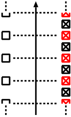
As we will see later, the effect of 𝒪⁡(ε){\mathcal{O}}(\varepsilon) will cancel the singular coefficient 1/ε1/\varepsilon of the Casimir operator 𝒯12ℭ\mathcal{T}^{\mathfrak{C}}_{12} in (4.4) and give a finite contribution. Therefore, the difference in the indices is very important. For this reason, although originally fermions have the indices of half-integers, if we want to compare fermions with bosons, we have to interpolate the indices into integers55 5 The important thing is to balance the bosonic indices with the fermionic ones. We can alternatively interpolate the bosonic indices into half-integers as another convention.. Note that fermions with integral indices do not exist in the representation space. We only introduce these states virtually for the comparison between bosons and fermions. (See Fig. 3.)
Refer to caption
bosonsfermions C
Figure 3: Virtual fermionic states with integer indices (Red). The other two dimensions of the weight lattice in Fig. 2 are omitted.

After interpolating the index of fermionic states into integers, the action of the bosonic generators reduces to

𝔓⁡|ϕna⟩=αi​[1−δ​γnγn]​(Dn+ε2​(xn+xn−1))​|ϕn+1a⟩,𝔓⁡|ψnα⟩=αi​(Dn+ε4​(xn+xn−1))​|ψn+1α⟩,\displaystyle{\mathfrak{P}}|\phi_{n}^{a}\rangle=\frac{\alpha}{i}\Bigl[1-\frac{\delta\gamma_{n}}{\gamma_{n}}\Bigr]\Bigl(D_{n}+\frac{\varepsilon}{2}(x_{n}+x_{n}^{-1})\Bigr)|\phi_{n+1}^{a}\rangle~,\quad{\mathfrak{P}}|\psi_{n}^{\alpha}\rangle=\frac{\alpha}{i}\left(D_{n}+\frac{\varepsilon}{4}(x_{n}+x_{n}^{-1})\right)|\psi^{\alpha}_{n+1}\rangle~,
ℭ⁡|ϕna⟩=12​(xn+xn−1)​Dn​|ϕna⟩,ℭ⁡|ψnα⟩=12​(xn+xn−1)​Dn​|ψnα⟩,\displaystyle{\mathfrak{C}}|\phi_{n}^{a}\rangle=\frac{1}{2}\bigl(x_{n}+x_{n}^{-1}\bigr)D_{n}|\phi^{a}_{n}\rangle~,\quad{\mathfrak{C}}|\psi_{n}^{\alpha}\rangle=\frac{1}{2}\bigl(x_{n}+x_{n}^{-1}\bigr)D_{n}|\psi^{\alpha}_{n}\rangle~,
𝔎⁡|ϕna⟩=iα​[1+δ​γnγn]​(Dn−ε​xn−1)​|ϕn−1a⟩,𝔎⁡|ψnα⟩=iα​(Dn−ε4​(xn+xn−1))​|ψn−1α⟩,\displaystyle{\mathfrak{K}}|\phi_{n}^{a}\rangle=\frac{i}{\alpha}\Bigl[1+\frac{\delta\gamma_{n}}{\gamma_{n}}\Bigr]\Bigl(D_{n}-\varepsilon x_{n}^{-1}\Bigr)|\phi_{n-1}^{a}\rangle~,\quad{\mathfrak{K}}|\psi_{n}^{\alpha}\rangle=\frac{i}{\alpha}\Bigl(D_{n}-\frac{\varepsilon}{4}(x_{n}+x_{n}^{-1})\Bigr)|\psi^{\alpha}_{n-1}\rangle~, (4.13)

where we have defined δ​γn=γn+1−γn\delta\gamma_{n}=\gamma_{n+1}-\gamma_{n}.

If we take the unitarity condition [7] into account, the variable γn\gamma_{n} is related to xnx_{n} by

g​γn=xn​Dn,\displaystyle\sqrt{g}\gamma_{n}=\sqrt{x_{n}D_{n}}~, (4.14)

which means δ​γn/γn=ε​xn−1​Dn−1/2\delta\gamma_{n}/\gamma_{n}=\varepsilon x_{n}^{-1}D_{n}^{-1}/2. In this case, the action of 𝔓{\mathfrak{P}} and 𝔎{\mathfrak{K}} is slightly simplified:

𝔓⁡|ϕna⟩=αi​(Dn+ε2​xn)​|ϕn+1a⟩,𝔎⁡|ϕna⟩=iα​(Dn−ε2​xn−1)​|ϕn−1a⟩.\displaystyle{\mathfrak{P}}|\phi_{n}^{a}\rangle=\frac{\alpha}{i}\left(D_{n}+\frac{\varepsilon}{2}x_{n}\right)|\phi^{a}_{n+1}\rangle~,\quad{\mathfrak{K}}|\phi_{n}^{a}\rangle=\frac{i}{\alpha}\left(D_{n}-\frac{\varepsilon}{2}x_{n}^{-1}\right)|\phi^{a}_{n-1}\rangle~. (4.15)

4.3 Classical r-matrix

After we constructed the representation in the previous subsection, let us reproduce the non-canonical terms of the classical r-matrix (4.1). We evaluate the singular term (4.6) explicitly on a two-site state |χn​χm′⟩|\chi_{n}\chi^{\prime}_{m}\rangle, defined by a tensor product |χn⟩1⊗|χm′⟩2|\chi_{n}\rangle_{1}\otimes|\chi^{\prime}_{m}\rangle_{2}:

1ε​𝒯12ℭ​|χn​χm′⟩=rn​|χn+1​χm−1′⟩+sn​|χn​χm′⟩+tn​|χn−1​χm+1′⟩,\displaystyle\frac{1}{\varepsilon}\mathcal{T}^{\mathfrak{C}}_{12}|\chi_{n}\chi^{\prime}_{m}\rangle=r_{n}|\chi_{n+1}\chi^{\prime}_{m-1}\rangle+s_{n}|\chi_{n}\chi^{\prime}_{m}\rangle+t_{n}|\chi_{n-1}\chi^{\prime}_{m+1}\rangle~, (4.16)

with rnr_{n}, sns_{n} and tnt_{n} being some appropriate coefficients. In general, we find the action of 𝒯12ℭ\mathcal{T}^{\mathfrak{C}}_{12} generates a linear combination of the states with different position indices. Comparing with the asymptotic state (2.10) which is a momentum eigenstate, it is not difficult to convince ourselves that we have to consider the eigenstate of 𝒯12ℭ\mathcal{T}^{\mathfrak{C}}_{12}. Therefore, let us solve the infinite-dimensional eigenvalue problem. Note that the reality condition of the eigenvalue is guaranteed only when the infinite-dimensional matrix (4.16) is symmetric. This is the case if we impose the unitarity condition (4.14).

Since generally a matrix has plural eigenvalues, we have to specify which eigenvalue or eigenstate we want to perturb from. In the classical limit g→∞g\to\infty of the 𝔰​𝔲​(2|2)\mathfrak{su}(2|2) spin chain, (2.18) gives x+=x−x^{+}=x^{-} which implies the excitation has the zero momentum p=0p=0 from (2.16). Hence, the asymptotic state (2.10) is simply the summation of states with excitations at each site with weight one. Motivated by this 𝔰​𝔲​(2|2)\mathfrak{su}(2|2) spin chain, we are led to studying the perturbation theory from the eigenstate summing up all the states with weight one,

∑l=−∞∞|χn−l​χm+l′⟩.\displaystyle\sum_{l=-\infty}^{\infty}|\chi_{n-l}\chi^{\prime}_{m+l}\rangle~. (4.17)

The solution to this eigenvalue problem is well-established in the perturbation theory of quantum mechanics [17]. In a system with Hamiltonian H(0)+ε​H(1)H^{(0)}+\varepsilon H^{(1)} where H(0)H^{(0)} is solved exactly to have the eigenvalue Eℓ(0)E^{(0)}_{\ell} with the eigenstate |φℓ(0)⟩|\varphi^{(0)}_{\ell}\rangle, the first-order deviation of the eigenvalue Eℓ(1)E^{(1)}_{\ell} is given by a famous formula,

Eℓ(1)=⟨φℓ(0)|H(1)|φℓ(0)⟩.\displaystyle E^{(1)}_{\ell}=\langle\varphi^{(0)}_{\ell}|H^{(1)}|\varphi^{(0)}_{\ell}\rangle~. (4.18)

In our present case where the eigenstate before the perturbation is a summation of weight one, the first-order deviation is simply given by summing up the matrix elements indiscriminately with weight one:

1ε​𝒯12ℭ​|χn​χm′⟩∼(rn+sn+tn)​|χn​χm′⟩.\displaystyle\frac{1}{\varepsilon}\mathcal{T}^{\mathfrak{C}}_{12}|\chi_{n}\chi^{\prime}_{m}\rangle\sim(r_{n}+s_{n}+t_{n})|\chi_{n}\chi^{\prime}_{m}\rangle~. (4.19)

After the calculation, we find (independently of δ​γ/γ\delta\gamma/\gamma)

1ε​𝒯12ℭ​|ϕ1a​ϕ2b⟩\displaystyle\frac{1}{\varepsilon}\mathcal{T}^{\mathfrak{C}}_{12}|\phi^{a}_{1}\phi^{b}_{2}\rangle =[1ε​T−12​(D1−1​D2+D1​D2−1)]​|ϕ1a​ϕ2b⟩,\displaystyle=\Bigl[\frac{1}{\varepsilon}T-\frac{1}{2}\left(D^{-1}_{1}D_{2}+D_{1}D^{-1}_{2}\right)\Bigr]|\phi^{a}_{1}\phi^{b}_{2}\rangle~,
1ε​𝒯12ℭ​|ψ1α​ψ2β⟩\displaystyle\frac{1}{\varepsilon}\mathcal{T}^{\mathfrak{C}}_{12}|\psi^{\alpha}_{1}\psi^{\beta}_{2}\rangle =[1ε​T+0]​|ψ1α​ψ2β⟩,\displaystyle=\Bigl[\frac{1}{\varepsilon}T+0\Bigr]|\psi^{\alpha}_{1}\psi^{\beta}_{2}\rangle~,
1ε​𝒯12ℭ​|ϕ1a​ψ2α⟩\displaystyle\frac{1}{\varepsilon}\mathcal{T}^{\mathfrak{C}}_{12}|\phi^{a}_{1}\psi^{\alpha}_{2}\rangle =[1ε​T−12​D1−1​D2]​|ϕ1a​ψ2α⟩,\displaystyle=\Bigl[\frac{1}{\varepsilon}T-\frac{1}{2}D^{-1}_{1}D_{2}\Bigr]|\phi^{a}_{1}\psi^{\alpha}_{2}\rangle~,
1ε​𝒯12ℭ​|ψ1α​ϕ2a⟩\displaystyle\frac{1}{\varepsilon}\mathcal{T}^{\mathfrak{C}}_{12}|\psi^{\alpha}_{1}\phi^{a}_{2}\rangle =[1ε​T−12​D1​D2−1]​|ψ1α​ϕ2a⟩,\displaystyle=\Bigl[\frac{1}{\varepsilon}T-\frac{1}{2}D_{1}D^{-1}_{2}\Bigr]|\psi^{\alpha}_{1}\phi^{a}_{2}\rangle~, (4.20)

where TT is a quantity of 𝒪⁡(1){\mathcal{O}}(1),

T=12​(x1+x1−1)​(x2+x2−1)​D1​D2−2​D1​D2,\displaystyle T=\dfrac{1}{2}(x_{1}+x^{-1}_{1})(x_{2}+x^{-1}_{2})D_{1}D_{2}-2D_{1}D_{2}~, (4.21)

and we have dropped higher order terms of ε\varepsilon. Since the variables associated to the 11-st and 22-nd excitations always have the position indices nn and mm, here we have used the “wavepacket” indices 11 and 22 instead of the position indices. By subtracting the average of the right-hand-sides, we can normalize the classical r-matrix as

1ε​𝒯12ℭ​|ϕ1a​ϕ2b⟩\displaystyle\frac{1}{\varepsilon}\mathcal{T}^{\mathfrak{C}}_{12}|\phi^{a}_{1}\phi^{b}_{2}\rangle =[−14​D1−1​D2−14​D1​D2−1]​|ϕ1a​ϕ2b⟩,\displaystyle=\Bigl[-\frac{1}{4}D^{-1}_{1}D_{2}-\frac{1}{4}D_{1}D^{-1}_{2}\Bigr]|\phi^{a}_{1}\phi^{b}_{2}\rangle~,
1ε​𝒯12ℭ​|ψ1α​ψ2β⟩\displaystyle\frac{1}{\varepsilon}\mathcal{T}^{\mathfrak{C}}_{12}|\psi^{\alpha}_{1}\psi^{\beta}_{2}\rangle =[+14​D1−1​D2+14​D1​D2−1]​|ψ1α​ψ2β⟩,\displaystyle=\Bigl[+\frac{1}{4}D^{-1}_{1}D_{2}+\frac{1}{4}D_{1}D^{-1}_{2}\Bigr]|\psi^{\alpha}_{1}\psi^{\beta}_{2}\rangle~,
1ε​𝒯12ℭ​|ϕ1a​ψ2α⟩\displaystyle\frac{1}{\varepsilon}\mathcal{T}^{\mathfrak{C}}_{12}|\phi^{a}_{1}\psi^{\alpha}_{2}\rangle =[−14​D1−1​D2+14​D1​D2−1]​|ϕ1a​ψ2α⟩,\displaystyle=\Bigl[-\frac{1}{4}D^{-1}_{1}D_{2}+\frac{1}{4}D_{1}D^{-1}_{2}\Bigr]|\phi^{a}_{1}\psi^{\alpha}_{2}\rangle~,
1ε​𝒯12ℭ​|ψ1α​ϕ2a⟩\displaystyle\frac{1}{\varepsilon}\mathcal{T}^{\mathfrak{C}}_{12}|\psi^{\alpha}_{1}\phi^{a}_{2}\rangle =[+14​D1−1​D2−14​D1​D2−1]​|ψ1α​ϕ2a⟩.\displaystyle=\Bigl[+\frac{1}{4}D^{-1}_{1}D_{2}-\frac{1}{4}D_{1}D^{-1}_{2}\Bigr]|\psi^{\alpha}_{1}\phi^{a}_{2}\rangle~. (4.22)

This is nothing but the non-canonical terms of the AdS/CFT classical r-matrix (4.1).

Since we are solving an infinite-dimensional eigenvalue problem, it is safer to present the eigenstates as well, instead of simply applying the formula (4.18) from the perturbation theory. For this purpose we have to know that rnr_{n}, sns_{n} and tnt_{n} appeared above satisfy

sn+1−sn=−u1​D1+u2​D2,rn+1−rn=tn+1−tn=12​(u2​D1−u1​D2),\displaystyle s_{n+1}-s_{n}=-u_{1}D_{1}+u_{2}D_{2}~,\quad r_{n+1}-r_{n}=t_{n+1}-t_{n}=\frac{1}{2}(u_{2}D_{1}-u_{1}D_{2})~, (4.23)

with the spectral parameter u=x+x−1u=x+x^{-1}. This recursive relation is independent of the states in the representation space, because it comes from the universal singular term TT (4.21). If we assume the eigenstate to be

|χ1​χ2′⟩=∑l=−∞∞(1+ε​fn−l)​|χn−l​χm+l′⟩,\displaystyle|\chi_{1}\chi^{\prime}_{2}\rangle=\sum_{l=-\infty}^{\infty}(1+\varepsilon f_{n-l})|\chi_{n-l}\chi^{\prime}_{m+l}\rangle~, (4.24)

we will find a recursive relation for fnf_{n} independent of bosons or fermions:

fn+1−2​fn+fn−1=f1−2​f0+f−1+n⁡(u2−u1)​(D1−1+D2−1).\displaystyle f_{n+1}-2f_{n}+f_{n-1}=f_{1}-2f_{0}+f_{-1}+n(u_{2}-u_{1})(D_{1}^{-1}+D_{2}^{-1})~. (4.25)

The recursive relation can be solved by

fn=n36​(u2−u1)​(D1−1+D2−1),\displaystyle f_{n}=\frac{n^{3}}{6}(u_{2}-u_{1})(D_{1}^{-1}+D_{2}^{-1})~, (4.26)

with suitable initial conditions. It is easy to reproduce the above eigenvalues from this eigenvector. We thus complete our solution to the eigenvalue problem.

5 Conclusions

In this paper, we have investigated the AdS/CFT spin chain with the symmetry 𝔭​𝔰​𝔲​(2|2)⋉ℝ3\mathfrak{psu}(2|2)\ltimes{\mathbb{R}}^{3} using the exceptional Lie superalgebra 𝔡⁡(2,1,ε)\mathfrak{d}(2,1;\varepsilon). In our analysis, we have obtained two results. First, we have rederived the coproducts of the level-1 Yangian generators from 𝔡⁡(2,1,ε)\mathfrak{d}(2,1;\varepsilon). In the derivation, we find that the non-trivial part of the secret symmetry ℑ{\mathfrak{I}} appears as the ε\varepsilon-correction of the last 𝔰​𝔲​(2)\mathfrak{su}(2) triplet generators ℭ𝔞𝔟{\mathfrak{C}}^{\mathfrak{a}}{}_{\mathfrak{b}} in 𝔡⁡(2,1,ε)\mathfrak{d}(2,1;\varepsilon). Secondly we have reproduced the non-canonical AdS/CFT classical r-matrix (1.3) from the canonical r-matrix of 𝔡⁡(2,1,ε)\mathfrak{d}(2,1;\varepsilon). The non-canonical terms of the classical r-matrix come from the differences of the action of ℭ𝔞𝔟{\mathfrak{C}}^{\mathfrak{a}}{}_{\mathfrak{b}} on bosons and fermions.

Originally, as we explained in the introduction, three regularizations were adopted to cure the degeneracy of the Killing form: superalgebra 𝔡⁡(2,1,ε)\mathfrak{d}(2,1;\varepsilon), 𝔰​𝔲​(2)\mathfrak{su}(2) outer automorphism and superalgebra 𝔲⁡(2|2)\mathfrak{u}(2|2). The 𝔰​𝔲​(2)\mathfrak{su}(2) outer automorphism does not look intrinsic to the 𝔰​𝔲​(2|2)\mathfrak{su}(2|2) spin chain model. In our analysis, we have given an interpretation to all these regularizations in 𝔡⁡(2,1,ε)\mathfrak{d}(2,1;\varepsilon) and made the outer 𝔰​𝔲​(2)\mathfrak{su}(2) automorphism look more intrinsic to the model.

Let us conclude by listing several further directions.

  • •

    The super Yang-Mills theory does not have the symmetry 𝔡⁡(2,1,ε)\mathfrak{d}(2,1;\varepsilon). At this stage, pursuing the Yangian symmetries in 𝔡⁡(2,1,ε)\mathfrak{d}(2,1;\varepsilon) is a purely technical tool to access various results of the Yangian algebra with the non-degenerating Killing form and to study the secret symmetry as the ε\varepsilon-correction. However, considering the success of the off-shell formalism with the centrally extended 𝔰​𝔲​(2|2)\mathfrak{su}(2|2) algebra and the naturalness of reproduction of this algebra from 𝔡⁡(2,1,ε)\mathfrak{d}(2,1;\varepsilon) in the limit ε→0\varepsilon\to 0, it may be eventually possible to assign a physical meaning to the exceptional superalgebra 𝔡⁡(2,1,ε)\mathfrak{d}(2,1;\varepsilon) in the super Yang-Mills theory (or its deformation).

  • •

    Although our derivation of the AdS/CFT classical r-matrix from the exceptional superalgebra 𝔡⁡(2,1,ε)\mathfrak{d}(2,1;\varepsilon) fully makes sense from the viewpoint of the representation theory, it is not easy to assign a physical interpretation to the 𝔡⁡(2,1,ε)\mathfrak{d}(2,1;\varepsilon) spin chain. Especially, it is not very clear whether the mathematical tensor product of the single-excitation states really corresponds to the physical picture of a spin chain state with multi-excitations. Since the representation of 𝔡⁡(2,1,ε)\mathfrak{d}(2,1;\varepsilon) has the position index, making full sense of the 𝔡⁡(2,1,ε)\mathfrak{d}(2,1;\varepsilon) spin chain may be helpful in understanding the finite size effects [18]. Also, since we have subtracted the overall shift to derive the non-canonical expression of the classical r-matrix, we expect the 𝔡⁡(2,1,ε)\mathfrak{d}(2,1;\varepsilon) spin chain gives an implication to the overall phase factor [19].

  • •

    In section 3 we have reproduced the non-trivial coproduct of the symmetry ℑ{\mathfrak{I}} as the ε\varepsilon-correction of the generator ℭ{\mathfrak{C}}, while the non-canonical term of the AdS/CFT classical r-matrix seems to be reproduced directly from the ε\varepsilon-correction of the generators 𝔓{\mathfrak{P}} and 𝔎{\mathfrak{K}} in section 4. We believe that the difference is “convention-dependent”, though we cannot make this statement more clear. A similar question whether we can construct a secret symmetry with the non-trivial coproduct being ϵa​bϵα​β𝔔αa𝒰+1⊗𝔔βb\epsilon^{ab}\epsilon_{\alpha\beta}{\mathfrak{Q}}^{\alpha}{}_{a}{\mathcal{U}}^{+1}\otimes{\mathfrak{Q}}^{\beta}{}_{b} or ϵα​βϵa​b𝔖aα𝒰−1⊗𝔖bβ\epsilon^{\alpha\beta}\epsilon_{ab}{\mathfrak{S}}^{a}{}_{\alpha}{\mathcal{U}}^{-1}\otimes{\mathfrak{S}}^{b}{}_{\beta} [10] remains unanswered.

  • •

    Though various deformations are introduced to investigate the 𝔰​𝔲​(2|2)\mathfrak{su}(2|2) spin chain [20], our work suggests that we can lift the question of the universal R-matrix of the AdS/CFT spin chain into that of the exceptional superalgebra 𝔡⁡(2,1,ε)\mathfrak{d}(2,1;\varepsilon). Work on the universal R-matrix of 𝔡⁡(2,1,ε)\mathfrak{d}(2,1;\varepsilon) [21] seems promising in finding the universal R-matrix of the AdS/CFT spin chain.

  • •

    As we have mentioned in the introduction, two possible viewpoints can be assigned to the secret symmetry ℑ{\mathfrak{I}}: as the 𝔰​𝔲​(2)\mathfrak{su}(2) automorphism and as the composite operator 𝒯𝔭​𝔰​𝔲​ℭ−1\mathcal{T}^{\mathfrak{psu}}{\mathfrak{C}}^{-1}. In lifting the AdS/CFT spin chain to the 𝔡⁡(2,1,ε)\mathfrak{d}(2,1;\varepsilon) model, we believe we have given both ℑ{\mathfrak{I}} and 𝔅𝔞𝔟{\mathfrak{B}}^{\mathfrak{a}}{}_{\mathfrak{b}} a nice picture as the ε\varepsilon-correction of the last 𝔰​𝔲​(2)\mathfrak{su}(2) generators ℭ𝔞𝔟{\mathfrak{C}}^{\mathfrak{a}}{}_{\mathfrak{b}}. However, it is still unclear how the interpretation as a composite operator is consistent from the 𝔡⁡(2,1,ε)\mathfrak{d}(2,1;\varepsilon) viewpoint. Understanding the meaning of the composite operator interpretation may help us in deriving the non-canonical classical r-matrix from 𝔡⁡(2,1,ε)\mathfrak{d}(2,1;\varepsilon) at the algebraic level without mentioning to the representation.

  • •

    It is always interesting to study various aspects of this spin chain model from the string worldsheet theory. Recent works [22] may give a clue in this direction.

Acknowledgement

We are grateful to H. Awata, H.Y. Chen, A. Hashimoto, H. Hayashi, N. Ishibashi, Y. Satoh, S. Teraguchi, Y. Yonezawa, especially our colleague H. Kanno and our previous collaborator A. Torrielli for valuable discussions. Part of this work was done during “The 2nd Asian Winter School on String Theory” at Kusatsu in Japan. We would also like to thank the lecturers S. Minwalla and M. Staudacher for patiently answering our basic questions related to the subject of this paper. We are also grateful to N. Beisert and F. Spill for their valuable comments on the previous version of this paper. The work of S.M. is supported partly by Inamori Foundation and partly by Grant-in-Aid for Young Scientists (B) [#18740143] from the Japan Ministry of Education, Culture, Sports, Science and Technology.

References

  • [1] J. A. Minahan and K. Zarembo, “The Bethe-ansatz for N = 4 super Yang-Mills,” JHEP 0303, 013 (2003) [arXiv:hep-th/0212208].
  • [2] I. Bena, J. Polchinski and R. Roiban, “Hidden symmetries of the AdS(5) x S**5 superstring,” Phys. Rev. D 69, 046002 (2004) [arXiv:hep-th/0305116].
  • [3] N. Beisert, “The dilatation operator of N = 4 super Yang-Mills theory and integrability,” Phys. Rept. 405, 1 (2005) [arXiv:hep-th/0407277]. A. A. Tseytlin, “Semiclassical strings and AdS/CFT,” arXiv:hep-th/0409296. J. Plefka, “Spinning strings and integrable spin chains in the AdS/CFT correspondence,” Living Rev. Rel. 8, 9 (2005) [arXiv:hep-th/0507136]. J. A. Minahan, “A Brief Introduction To The Bethe Ansatz In N=4 Super-Yang-Mills,” J. Phys. A 39, 12657 (2006).
  • [4] N. Beisert, “The s​u​(2|2)su(2|2) dynamic S-matrix,” arXiv:hep-th/0511082.
  • [5] A. A. Belavin and V. G. Drinfel’d, “Solutions of the classical Yang-Baxter equation for simple Lie algebras,” Funct. Anal. Appl. 16 159 (1982).
  • [6] Z. Q. Ma, “Yang-Baxter equation and quantum enveloping algebras,” Advanced series on theoretical physical science, World Scientific (1993). N. J. MacKay, “Introduction to Yangian symmetry in integrable field theory,” Int. J. Mod. Phys. A 20, 7189 (2005) [arXiv:hep-th/0409183].
  • [7] N. Beisert, “The Analytic Bethe Ansatz for a Chain with Centrally Extended s​u​(2|2)su(2|2) Symmetry,” J. Stat. Mech. 0701, P017 (2007) [arXiv:nlin/0610017].
  • [8] S. Moriyama and A. Torrielli, “A Yangian Double for the AdS/CFT Classical r-matrix,” JHEP 0706, 083 (2007) [arXiv:0706.0884 [hep-th]].
  • [9] T. Matsumoto, S. Moriyama and A. Torrielli, “A Secret Symmetry of the AdS/CFT S-matrix,” JHEP 0709, 099 (2007) [arXiv:0708.1285 [hep-th]].
  • [10] N. Beisert and F. Spill, “The Classical r-matrix of AdS/CFT and its Lie Bialgebra Structure,” arXiv:0708.1762 [hep-th].
  • [11] C. Gomez and R. Hernandez, “The magnon kinematics of the AdS/CFT correspondence,” JHEP 0611, 021 (2006) [arXiv:hep-th/0608029]. J. Plefka, F. Spill and A. Torrielli, “On the Hopf algebra structure of the AdS/CFT S-matrix,” Phys. Rev. D 74, 066008 (2006) [arXiv:hep-th/0608038].
  • [12] G. Arutyunov and S. Frolov, “On AdS(5) x S**5 string S-matrix,” Phys. Lett. B 639, 378 (2006) [arXiv:hep-th/0604043].
  • [13] A. Torrielli, “Classical r-matrix of the s​u​(2|2)su(2|2) SYM spin-chain,” Phys. Rev. D 75, 105020 (2007) [arXiv:hep-th/0701281].
  • [14] N. Beisert, “The S-Matrix of AdS/CFT and Yangian Symmetry,” PoS SOLVAY, 002 (2006) [arXiv:0704.0400 [nlin.SI]].
  • [15] J. Van Der Jeugt, “Irreducible Representations Of The Exceptional Lie Superalgebras D⁡(2,1,α)D(2,1;\alpha),” J. Math. Phys. 26, 913 (1985).
  • [16] F. Spill, “Hopf Algebras in the AdS/CFT Correspondence”, Diploma Thesis, Humboldt University of Berlin, 2007.
  • [17] J. J. Sakurai, “Modern Quantum Mechanics”, Addison-Wesley Publishing Company (1993). K. Igi, H. Kawai, “Quantum Mechanics”, Kodansha (1994), in Japanese.
  • [18] J. Ambjorn, R. A. Janik and C. Kristjansen, “Wrapping interactions and a new source of corrections to the spin-chain / string duality,” Nucl. Phys. B 736, 288 (2006) [arXiv:hep-th/0510171]. G. Arutyunov, S. Frolov and M. Zamaklar, “Finite-size effects from giant magnons,” Nucl. Phys. B 778, 1 (2007) [arXiv:hep-th/0606126]. R. A. Janik and T. Lukowski, “Wrapping interactions at strong coupling – the giant magnon,” Phys. Rev. D 76, 126008 (2007) [arXiv:0708.2208 [hep-th]]. G. Arutyunov and S. Frolov, “On String S-matrix, Bound States and TBA,” JHEP 0712, 024 (2007) [arXiv:0710.1568 [hep-th]]. Y. Hatsuda and R. Suzuki, “Finite-Size Effects for Dyonic Giant Magnons,” arXiv:0801.0747 [hep-th]. J. A. Minahan and O. Ohlsson Sax, “Finite size effects for giant magnons on physical strings,” arXiv:0801.2064 [hep-th].
  • [19] R. A. Janik, “The AdS(5) x S**5 superstring worldsheet S-matrix and crossing symmetry,” Phys. Rev. D 73, 086006 (2006) [arXiv:hep-th/0603038]. N. Beisert, R. Hernandez and E. Lopez, “A crossing-symmetric phase for AdS(5) x S**5 strings,” JHEP 0611, 070 (2006) [arXiv:hep-th/0609044]. N. Beisert, B. Eden and M. Staudacher, “Transcendentality and crossing,” J. Stat. Mech. 0701, P021 (2007) [arXiv:hep-th/0610251]. K. Sakai and Y. Satoh, “Microscopic formulation of the S-matrix in AdS/CFT,” JHEP 0712, 044 (2007) [arXiv:0709.3342 [hep-th]].
  • [20] N. Beisert and P. Koroteev, “Quantum Deformations of the One-Dimensional Hubbard Model,” arXiv:0802.0777 [hep-th].
  • [21] I. Heckenberger, F. Spill, A. Torrielli and H. Yamane, “Drinfeld second realization of the quantum affine superalgebras of D(1)(2,1:x)D^{(1)}(2,1:x) via the Weyl groupoid,” arXiv:0705.1071 [math.QA].
  • [22] G. Arutyunov, S. Frolov, J. Plefka and M. Zamaklar, “The off-shell symmetry algebra of the light-cone AdS(5) x S**5 superstring,” J. Phys. A 40, 3583 (2007) [arXiv:hep-th/0609157]. T. Klose, T. McLoughlin, R. Roiban and K. Zarembo, “Worldsheet scattering in AdS(5) x S**5,” JHEP 0703, 094 (2007) [arXiv:hep-th/0611169]. A. Mikhailov and S. Schafer-Nameki, “Algebra of transfer-matrices and Yang-Baxter equations on the string worldsheet in AdS(5) x S(5),” arXiv:0712.4278 [hep-th]. J. M. Evans and J. O. Madsen, “Quantum integrability of coupled N = 1 super sine/sinh-Gordon theories and the Lie superalgebra D⁡(2,1,α)D(2,1,\alpha),” Int. J. Mod. Phys. A 14, 2551 (1999) [arXiv:hep-th/9712227].