Les Houches Lectures on Constructing String Vacua
Jefferson Physical Laboratory, Harvard University,
Cambridge, MA 02138, USA
and
Instituut voor Theoretische Fysica, KU Leuven,
Celestijnenlaan 200D, B-3001 Leuven, Belgium
Photo: width 7.5cm height 11cm
Contents
Abstract: These lectures give a detailed introduction to constructing and analyzing string vacua suitable for phenomenological model building, with particular emphasis on F-theory flux vacua. Topics include (1) general challenges and overview of some proposed scenarios, (2) an extensive introduction to F-theory and its relation to M-theory and perturbative IIB string theory, (3) F-theory flux vacua and moduli stabilization scenarios, (4) a practical geometrical toolkit for constructing string vacua from scratch, (5) statistics of flux vacua, and (6) explicit models.
1 Introduction
The real world as we know it happens at energies well below the Planck scale, so it is very well described by effective field theory. There is a continuous infinity of consistent effective field theories. Remarkably, only a measure zero fraction of those seems to be obtainable from string theory. These effective field theories arise as low energy descriptions of certain “vacua” of string theory, which in some approximations schemes can be thought of as solutions to the equations of motion for the compactification space. Constraints on low energy effective particle spectra and interactions then typically arise from topological constraints on the internal degrees of freedom. Discreteness of the allowed values of parameters in the low energy effective action often arises from quantization effects, such as quantization of internal magnetic fluxes.
It is this remarkable selectivity of string theory which fuels the field known as string phenomenology. If the constraints from requiring the existence of a string theory UV completion are strong enough, then this can take us a significant step beyond the theorizing we can do based on field theory alone. This prompts the question: Are UV completion constraints merely academically fascinating, or are they strong enough to lead to experimental predictions?
In part triggered by developments in constructing string vacua meeting a number of rough observational constraints, a hypothetical picture has emerged in which the real world as we know it is just a tiny patch in a vast, eternally inflating multiverse, which effectively samples an gargantuan “landscape” of string vacua [1]. If correct, this has profound implications for a number of paradigms in physics, including the notion of naturalness and how we should read some of the stunning fine tunings of parameters in nature, as explained by Nima Arkani-Hamed at this school. The string theory landscape picture is not uncontested [2], and prompts the question: Is it correct?
We are far from a systematic understanding of the Hilbert space(s) of string theory, or even the space of its approximate, semiclassical vacua with four large dimensions. In view of this, one might consider the above questions premature. Nevertheless, we do understand parts. This includes in particular AdS vacua which have a known dual CFT description, and, to some extent at least, approximate semiclassical vacua which can be constructed as solutions to the classical equations of motion in regimes where quantum corrections are small. The former class is not immediately useful yet as a description of the universe as we know it, as observations indicate our vacuum has a positive effective cosmological constant. We can however try to construct controlled vacua of the latter kind, and address within this class the general questions raised above, even if our vacuum might not be accessible in this way.
The main goal of these lectures is to provide a detailed introduction to the best studied and for phenomenological applications richest set of such approximate semiclassical vacua: type IIB flux compactifications. I will almost exclusively focus on the formal construction of these vacua in string theory and the development of general methods for their analysis, leaving out specific phenomenological applications. I felt this would best complement the existing literature, and be most likely to be useful in the long run. The path from string theory to the real world is long and twisted, and if we want to get beyond loosely string-inspired but further unconstrained effective field theories, there is no choice but to dive deep into the bowels of string theory itself.
I have tried to make the lectures more or less self-contained. In particular all of the geometrical tools needed to build actual models are introduced from scratch, assuming only basic knowledge of the differential geometry contained in section 2 of [3]. The framework in which I will be working is the F-theory description of IIB theory, because for many applications this is the most powerful and versatile approach, including for constructing semi-realistic string vacua. Nevertheless, as far as I know, no extensive elementary introduction bringing together all the basic ideas needed for applications of constructing F-theory vacua is available in the literature. I have therefore devoted a significant part of these lectures to explaining what F-theory is, how precisely it relates to M-theory and to the weak coupling limit of type IIB string theory, and how flux vacua and their number distributions over parameter space are obtained in this framework.
By the end of these lectures, you should be able to construct and analyze your own string vacuum.
The outline of this extended write-up is as follows:
- 1.
In section 2, I outline some of the main challenges that arise when trying to construct controlled string vacua (of any kind, not just IIB) and give a brief overview of several of the scenarios that have been proposed. In particular I will explain why successful explicit constructions must be “dirty”, involving many ingredients which might seem unnecessarily contrived at first sight.
- 2.
In section 3, I explain what F-theory is, give its detailed construction in M-theory, discuss ways to think about branes, fluxes and tadpoles in this framework, explain how in general perturbative type IIB orientifold compactifications arise as a particular weak coupling limit, and how in this limit localized D7-branes and their worldvolume gauge fields emerge. I have tried to be as explicit as possible, following an elementary physical approach rather than an algebraic geometrical one.
- 3.
In section 4 we turn to the construction of F-theory flux vacua. First the four dimensional low energy effective action is given, both in the the general F-theory setting and in its perturbative IIB weak coupling limit. Next the effect of turning on fluxes is considered, how they induce an effective superpotential stabilizing the shape and 7-brane moduli and how they can produce strong warping effects. Fluxes leave the size moduli massless at tree level. The latter can get lifted by various quantum effects, which are discussed next. Finally, two concrete scenarios to achieve fully moduli stabilized vacua with small positive cosmological constant are reviewed, the KKLT [4] and large volume [5] scenarios.
- 4.
To find and analyze actual interesting concrete models of either of these two scenarios, a number of geometrical tools is needed. These are introduced from scratch in the hands-on geometrical toolbox which makes up section 5.
- 5.
Another indispensable ingredient in constructing and analyzing these vacua are techniques for computing approximate distributions of flux vacua over parameter space. These techniques are introduced and explained in quite a bit of detail in section 6, including a general abstract derivation of the continuum index approximation to counting zeros of ensembles of vector fields, which can then be applied to various flux vacua counting problems, including F-theory flux vacua. A summary is given of various results, and the section concludes with a short discussion of metastability, landscape population and probabilities in the context of flux vacua.
- 6.
Finally, in section 7, we put all of these basic results together and outline how explicit models of moduli stabilized F-theory flux vacua can be obtained.
The different sections can to a large extent be read independently, and readers only interested in certain aspects of the constructions can probably safely skip sections.
Finally, let me emphasize that these lecture notes are in no way supposed to be a comprehensive review of the subject. The references are not meant to reflect proper historical attribution and are seriously incomplete. They are merely intended to provide pointers to articles which can be used as a starting point for further reading.
2 Basics of string vacua
2.1 Why string vacua are dirty
Even if you have never gotten your hands dirty constructing semi-realistic string vacua yourself, you probably have heard or read [6] that they tend to have a certain Rube Goldberg [7] flavor to them. In the following I will sketch what the challenges are to construct such vacua in a reasonably controlled way, and how meeting these challenges unavoidably requires adding several layers of complications.
2.1.1 The Dine-Seiberg problem
Perturbative supersymmetric string theories in flat Minkowski space and weakly curved deformations thereof only exist in ten dimensions. Observations on the other hand suggest only four large, weakly curved dimensions. The most obvious way out of this conundrum is to consider string theory on a space of the form
| (2.1) |
where corresponds to visible space and a compact manifold sufficiently small to have escaped detection so far. The size of the space could be of the order of the fundamental scale, it could be highly curved and even defy classical notions of geometry, and it could break supersymmetry at a very high scale. Currently available techniques to analyze such situations are limited. Therefore the sensible thing to do is to consider well controlled cases and hope that these either will be favored by nature too, or that at least we can draw valuable lessons from them.
The most obvious well controlled cases are provided by compactifications (2.1) for which is large compared to the fundamental scale, and for which supersymmetry is broken at a scale well below the compactification scale. The latter is most easily achieved by first constructing a compactification which preserves some supersymmetry, and then perturb this in a controlled way to break supersymmetry.
In this regime, we can use the long distance, low energy approximation to string theory, that is, ten dimensional supergravity, described by an effective action for the massless fields. We can also consider eleven dimensional supergravity, the low energy approximation to M-theory [8], of which perturbative string theory is believed to be a particular weak coupling limit. Formally we can even go up one more dimension and imagine twelve dimensional F-theory [9], although this can be thought of more conservatively as a convenient geometrized description of type IIB string theory.
The following compactifications of string/M/F theory give rise to supersymmetry in four dimensional Minkowski space:
- 1.
heterotic or type I string theory on a three complex dimensional Calabi-Yau manifold
- 2.
type II string theory on a 3d Calabi-Yau orientifold
- 3.
M-theory on a holonomy manifold
- 4.
F-theory on a Calabi-Yau fourfold.
All of these compactification manifolds are Ricci flat to leading order at large volume.
However, such compactifications immediately present a problem: at tree level, i.e. classically, they always come with moduli. Moduli are deformations of the compactification which do not change the 4d effective energy and therefore correspond to massless scalars in four dimensions. For example the size of the compactification manifold is always a modulus at tree level, due to the scale invariance of vacuum Einstein equations. Other possible moduli are
- 1.
The dilaton , for all string theories. This is already a modulus of the ten dimensional theory in Minkowski space. It is the parameter controlling the worldsheet perturbative expansion of the theory.
- 2.
Axions: These arise when the supergravity theory under consideration has -form potentials and has nontrivial harmonic -forms (or equivalently nontrivial -cycles ), as adding such a harmonic -form to will not affect the field strength and hence not affect the energy. On the other hand adding a generic harmonic form is not a gauge transformation either, so these are physical, massless modes in the 4d theory.
- 3.
Metric moduli:
- (a)
CY complex structure (or shape) moduli, analogous to the complex structure modulus of the two-torus .
- (b)
CY Kähler (or size) moduli, analogous to the overall size of the .
- (c)
structure (shape and size) moduli
- (a)
- 4.
Brane deformation and/or vector bundle moduli. Including branes or bundles is often forced upon us, both by tadpole cancelation constraints and by the phenomenological desire to have gauge bosons and charged matter in the theory that could reproduce the Standard Model.
In generic compactifications, there are thousands of these moduli. This is not good. Massless or very light scalars, if they couple at least with gravitational strength to matter, would be observed as long range “fifth” forces. No such forces have been observed. Moreover, it is difficult to allow for light scalars while preserving the successful predictions of standard cosmology.
Now, this would not seem to be such a big deal, since including quantum corrections, at least after breaking supersymmetry, are virtually guaranteed to give masses to the moduli, since there is in general nothing that protects scalars from becoming massive after supersymmetry is broken. However, one then runs into a universal problem of theoretical physics, which can be sloganized by saying that when corrections can be computed, they are not important, and when they are important, they cannot be computed. More concretely, the problem here is what is usually referred to as the Dine-Seiberg problem [10]. The argument is very simple. Let be a modulus such as the volume or the inverse string coupling , with the property that corresponds to the weakly coupled region where we trust our tree level low energy effective action. Then if, as expected, quantum corrections generate a potential in the 4d effective theory, this potential will satisfy
| (2.2) |
precisely because of our assumption that at , we can trust the tree level low energy effective action, which has zero potential for , by definition, since is a modulus at tree level.

There are then two possibilities, as shown in figure 1 on the left: either at large , in which case the scalar has a runaway direction to , or at large , in which case the scalar is pulled to the strong coupling region. A local minimum can only arise if higher order corrections are included; one needs two more corrections for the first case and one more for the second, as illustrated in fig. 1 on the right. But, tautologically, when these corrections are important enough to cause a significant departure from the first order shape of , as is necessary to get a local minimum, one is no longer in the weakly coupled region, and in principle all higher order corrections might be important too. In the absence of extended supersymmetry ( in 4d), we generally lack the tools to compute more than a few orders in perturbation theory, so unavoidably we lose control.
On these grounds, Dine and Seiberg concluded in 1985 that the string vacuum we live in is probably strongly coupled. They may very well be right.
2.1.2 Flux vacua and no-go theorems
But new developments since then have changed the outlook somewhat. A crucial ingredient in these developments was the idea that by turning on -form magnetic fluxes in the internal manifold , many new string vacua could be designed [11]. Dirac quantization requires these fluxes to be integrally quantized, that is, integrals over closed -cycles must be integral (for a suitable normalization of ). So fluxes are discrete degrees of freedom. The type of flux and the possible values of depend on the theory under consideration, but the basic idea is always the same. The crucial point is that turning on flux generates a moduli potential at tree level, of the form11 1 For simplicity of exposition we suppress for now the additional dilaton dependence which we get in string theory (which is different for the two types of flux one can turn on, RR and NSNS). We work in units in which the 10/11 dimensional Planck scale is set to one.
| (2.3) |
where is the four dimensional Planck mass and is the volume of . The prefactor appears in the effective potential after rescaling the 4d metric as to remove the -dependence of the Einstein-Hilbert term in the 4d effective action.
Since the internal metric depends on the moduli we originally had, we thus generate a tree level potential for the moduli. This is great, but unfortunately does not solve our problem. Under a rescaling of the internal metric, the potential scales as , so if we parametrize the internal metric by where we normalize such that , we get
| (2.4) |
This is manifestly positive definite, so there is a runaway direction towards large , except if . This conclusion remains unchanged if we have different sets of fluxes with different values of , since each term will be positive definite. Now, if and the geometry is nonsingular, then positive definiteness of the internal metric implies , so there was no potential to begin with. Thus we conclude that in the regime in which classical geometry can be trusted, there can be no such flux vacua.
This analysis is a little too naive though. We neglected the possible backreaction of the fluxes on our originally Ricci-flat metric on . If the Einstein-Hilbert action of becomes nonzero, this will give an additional effective potential term in four dimensions, which will also scale under :
| (2.5) |
If the internal curvature is negative, the runaway gets only worse. So let us take it to be positive, as is the case for example for a sphere. If is nonzero only for , the curvature will in fact give the dominant contribution at large . We are then in the case of the dashed line in figure 1, and we see that flux vacua with negative cosmological constant might be possible. Indeed, such flux vacua are abundant. A subset are the so-called Freund-Rubin vacua [12], where and is taken to be an Einstein space; the simplest example is M-theory on AdS with 7-form flux on the . We will discuss these in more detail in the next subsection. However, such compactifications cannot be viewed as deformations of the compactifications to flat Minkowski space we started off with: The flux is what supports the internal manifold ; if we send to zero, collapses to zero size. You can see this from (2.5) from the fact that the minimum when scaling to zero keeping fixed, or explicitly for example for AdS, where the size of the (and, pegged to it, the curvature radius of AdS4) is proportional to a positive power of . Moreover, in examples studied so far, the KK scale is of order of the AdS scale. If this is so, then to get to our observed near-zero value of the cosmological constant, some quantum effect has to provide an additional contribution to the effective potential of the order of the KK scale, which tautologically means quantum corrections are not small compared to our leading order potential, and we lose control again. To see this correlation between the scales, note that
| (2.6) | |||||
| (2.7) | |||||
| (2.8) |
Here is the local minimum of , is the diameter22 2 The diameter is the largest distance between two points. Its relation to the KK scale, i.e. the bottom of the eigenvalue spectrum of the Laplacian, is intuitively plausible but mathematically not trivial. See [13] for further discussion. of for the metric , and is the diameter for the metric . For the round sphere, (2.8) is of order 1, and it appears difficult to find examples where this scale ratio can be made very small. I don’t known of a proof that this cannot be done though. If you looked a little harder, you might well be able to find constructions with a large scale hierarchy. We will briefly return to these compactifications in the next subsection.
So far we discussed the cases with . When only (i.e. a nonzero scalar gradient), things are qualitatively different. Now the two terms in (2.5) scale in the same way, so if the curvature can adjust itself so the two terms cancel at a given , they will cancel at all , and the potential will be zero. Such solutions do exist in type IIB theory. A simple example is with 24 7-branes transversal to the , which source RR 1-form flux . More generally, F-theory compactifications can be thought of as being of this kind. We will discuss these in detail further on. Still, such compactifications do not solve our problem. By construction, the overall scale modulus remains massless. On top of that, there will be other nonstabilized geometric moduli — a typical F-theory compactification for example has thousands of moduli.
When , the dominant term in (2.5) at is the corresponding flux term. Together with other flux terms, this could in principle lead to the situation corresponding to the solid line in fig. 1, and could thus possibly even lead to metastable Minkowski or de Sitter vacua. We will return to this case shortly.
The above arguments are a baby version of a very general no-go theorem, proven by Maldacena and Nuñez [14] (see also [15] and recently [16]). The theorem can be stated as follows. We start with any dimensional gravity theory whose gravitational dynamics is given by the standard Einstein-Hilbert action (without higher curvature corrections), coupled to arbitrary massless fields (scalars, -forms, nonabelian gauge fields, …) with positive kinetic terms, and with zero or negative potential (which could depend on the scalars). We then compactify this theory on a manifold , with coordinates , in the most general way, including a possible -dependent “warp factor” , to obtain a vacuum solution in dimensions:
| (2.9) |
By vacuum solution we mean a metric which is either Anti-de Sitter, Minkowski, or de Sitter. We assume that is compact and that the warp factor does not diverge anywhere.33 3 This is somewhat stronger than the conditions under which the theorem was proven in [14]. The theorem now says that under these conditions, there are no compactifications down to de Sitter space, and none to Minkowski space except if or , in which case we get Minkowski with constant.
This is consistent with our simple analysis above. (The case , which is related to by was not considered in our analysis because we restricted to magnetic fluxes, which have all legs in the internal space.)
As promised above, we now return to the case . This was studied separately in [14] for the particular string theory where it could occur, namely “massive” type IIA, with the conclusion that no compactifications to Minkowski or de Sitter can exist, dashing the hope left open by our simple scaling analysis earlier. A few AdS solutions with are known [17], but unfortunately they all have KK scales of the order of the AdS scale.
2.1.3 Orientifold planes and type II flux vacua
The Maldacena-Nuñez no-go theorem sounds like bad news, and in fact it is. Not because the assumptions of the theorem cannot be violated — string theory violates them immediately, because its low energy effective action does have higher order curvature corrections, and because the theory contains singular negative tension objects (O-planes) — but because it forces us to depart from the clean world of actions to second order in derivatives and smooth geometries, and to migrate to the dirty world of higher order corrections and orientifold singularities. As a result, control problems creep back in.
Still, let us proceed. We begin by returning to our simple scaling analysis, and add to (2.5) some of the extra contributions D-branes and O-planes provide. Space filling D-branes wrapping a -cycle in will give a contribution , while orientifold planes on a -cycle give a similar contribution but (possibly) negative. Curvature of D-branes typically gives a negative contribution to the energy density scaling like the energy of a D-brane. Worldvolume fluxes on D-branes give positive energy contributions scaling like those of lower dimensional branes.
Clearly now there are many more terms in the effective potential, include some more with negative signs, so we can expect to get minima more easily. We consider two special cases of interest. The first one is type IIB string theory on a Calabi-Yau orientifold with O3 and O7 planes, D3 and D7 branes, and NSNS () and RR () 3-form fluxes. Schematically this gives the potential
| (2.10) | |||||
Here we reinstated the dependence on the dilaton , and denotes the total tension from D and O branes in the metric and with . The structure of the potential suggests we can find nontrivial Minkowski flux vacua with , provided the D7 and O7 tensions cancel, so , and provided the contributions from fluxes, O3 and D3-branes cancel as well. Indeed such vacua turn out to exist [18, 19, 20], and we will discuss them in great detail in section 4.
Of course, by construction now, is still a modulus. In fact it turns out that all Kähler moduli remain unfixed by the flux potential. To stabilize those in this setup, one must resort to quantum corrections again, and the Dine-Seiberg problem kicks back in. Nevertheless an ingenious scenario for how this could be made to work in a reasonably controlled way, and moreover how a small positive cosmological constant could be achieved, was proposed by Kachru, Kallosh, Linde and Trivedi (KKLT) [4]. We will return to this in section 4.
The second case we consider is type IIA on a Calabi-Yau orientifold with O6 planes, order 1 units of RR flux and NSNS flux , and units of RR flux . Setting O(1) quantities to 1, this generates a potential of the form
| (2.11) |
The first negative term is the O6 contribution. Setting , this has minima for large at
| (2.12) |
that is, large volume and weak string coupling. In [23], a more refined analysis was done and it was shown that such flux vacua indeed exist in type IIA string theory, at least at the level of the 4d effective theory, with all geometric moduli fixed. In [24] this was promoted to full ten dimensional solutions in the approximation of smeared O6 charge. Although you cannot see this from the simple considerations we made, the minima turn out to be always AdS minima, but of a different nature than those of Freund-Rubin type we mentioned earlier. From the scaling (2.12), we see that , , and consequently
| (2.13) |
Hence, unlike in the Freund-Rubin case, provided the diameter of the unit volume normalized metric does not grow with (or grows less fast than ), we automatically get a hierarchy of KK and AdS scales in the large limit. This removes the immediate obstruction to controlled lifting to positive cosmological constant we mentioned for Freund-Rubin type vacua. Which is not to say that lifting is now straightforward or that there are no other control issues with these compactifications. We will come back to this in the next subsection.
In conclusion, we arrived at classical moduli stabilization scenarios in type IIB and IIA string theory which might have a chance of producing some reasonably controlled vacua. But they are not the simple smooth exact classical solutions we might have hoped for. The constructions we have at this point need many different ingredients. Calling them Rube Goldberg contraptions would be excusable. But as I hope I have made clear, it is the failures of simpler ideas44 4 and perhaps the strategy to start from the highly supersymmetric string vacua we do know and control. that has driven us this far.
2.2 A brief overview of some existing scenarios
We now turn to a brief overview of some of the constructions that have been proposed, and of their virtues and drawbacks. I will not try to be complete, far from it; the idea is to just give a flavor of what has been done and what the issues are. Several concepts mentioned may be foreign to you; some of the material will become more clear further on in the lectures. Much more can be found in the reviews [25, 26]. The references below are very incomplete and only meant to give you some pointers to the relevant clusters of papers.
2.2.1 IIB orientifolds / F-theory
These are variants of the KKLT scenario mentioned in the previous subsection. We will deeply get into the details of these scenarios in the next sections. Some key references for the basic setup are [18, 27, 19, 20, 4, 5]. The virtues of this scenario, when it works, are:
- +
Complex structure moduli, dilaton, D7 moduli can be stabilized classically at high mass scales by RR, NSNS and D7 worldvolume fluxes.
- +
Because there are always many more fluxes than moduli, there is a very high degree of discrete tunability of physical parameters, which helps in producing controlled models. In particular the cosmological constant can in principle be discretely tuned to become extremely small, easily of the order of the measured cosmological constant or less [28].
- +
The classical geometry of the compactification manifold remains Calabi-Yau after turning on fluxes, up to warping [20]. This means in particular that many of the powerful techniques from algebraic geometry, which were invaluable to get a handle on Calabi-Yau compactifications without fluxes, can still be used to describe these vacua.
- +
Strongly warped throats of Klebanov-Strassler type [29] can be achieved through the warping of the Calabi-Yau geometry. This can generate large scale hierarchies, useful for e.g. controlled supersymmetry breaking by adding anti-D3-branes at the bottom of the throat, or for embedding Randall-Sundrum [30] type scenarios in string theory.
- +
- +
There is a rich set of explicit D-brane constructions possible in these models, useful for particle physics model building; for a review see [34], and for a nice introductory overview see [35]. More general F-theory model building is also possible and provides probably the most extensive class of particle physics models in string theory, allowing in particular unification to arise naturally [21, 22].
- +
The F-theory description provides corrections to the geometry which smooth out the O7 singularities [36]. This is needed if one wants a large radius geometrical description of the background because O-plane singularities tend to be of a very bad kind, ripping up space at finite distance due to the negative tension of O-planes.
The main drawbacks are
- –
One needs quantum corrections to stabilize the Kähler (size) moduli, making the Dine-Seiberg problem something to worry about.
- –
Generic F-theory compactifications, away from special (orientifold) limits, do not have a globally well defined weakly coupled worldsheet description, even in the infinite volume limit, because the string coupling undergoes -duality transformations when circling around generic 7-branes. Hence for generic compactifications, it is unclear how to systematically compute e.g. corrections even in principle.
- –
Similarly, it is not known how to systematically compute such corrections in the presence of RR flux. This is a universal problem of any flux compactification involving RR fluxes.
2.2.2 IIA orientifolds
This is the IIA flux model mentioned at the end of the previous subsection. A key reference for the basic setup is [23]. The virtues of this scenario are
- +
Classical RR and NSNS fluxes are sufficient to stabilize all geometrical moduli, in what from the low energy effective action point of view at least appears to be a parametrically controlled regime. Axions are not lifted, but these can get masses by quantum effects without triggering control issues.
- +
Intersecting D-brane models can be embedded (although they are special Lagrangian, and very few explicit constructions of special Lagrangians in compact manifolds are known).
The drawbacks are:
- –
Because there are about as many moduli as fluxes, there is only limited discrete tunability. Warped throats cannot be generated classically, so controlled supersymmetry breaking by adding anti-D-branes is not possible in this way.
- –
The presence of the localized O6 makes the solutions geometrically incomplete, since the metric and string coupling blow up at finite radius from the O6. In flat space, this can be regularized by lifting to M-theory (the analog of lifting type IIB O7-planes to F-theory), where the O6 turns into the smooth Atiyah-Hitchin manifold [37]. Unfortunately, there is no direct M-theory lift in the case at hand, due to the presence of flux. The control issues this implies are further discussed in [38].
- –
2.2.3 M on
flux vacua can be viewed as M-theory uplifts of IIA orientifold flux vacua, but with . The latter restriction must be made because, although type IIA with (also known as massive type IIA or Romans theory) can be viewed as a limit of M-theory via reduction on a 2-torus and a twisted version of T-duality [41], it cannot be directly be obtained by compactification of eleven dimensional supergravity.
The good news is that everything is geometrical in this setup; in particular there are no orientifold planes to worry about. The bad news is that, in accordance with our general scaling arguments, the flux potential does not have local minima. (This agrees with the fact that in IIA, when , there are no vacua.)
Thus, a new ingredient is needed. In [42], a proposal was made for such a new ingredient, making use of constraints from supersymmetry, leading to a negative contribution to the potential from certain nonabelian excitations around a locus of singularities in the manifold. Although unfortunately no explicit example is known, and its physical origin remains to be elucidated, the virtue of such a model would be that it freezes all geometric moduli at once. The drawback, besides the fact that it is not known conclusively if such compactifications actually exist, are similar to those of type IIA models.
2.2.4 Pure flux
This includes all flux compactifications which exist without the addition of “extra” elements such as orientifold planes. The simplest class of examples are the supersymmetric Freund-Rubin vacua [12] of M-theory of the form AdS where is a Sasaki-Einstein 7-manifold (for reviews see [43, 44, 45]), supported by units of flux on . Sasaki-Einstein manifold are obtained as the base of Calabi-Yau fourfold cones. The simplest example is , obtained by considering eight dimensional flat space as a Calabi-Yau cone over a sphere.
Such vacua are very well controlled in the large limit, and have 2+1 dimensional superconformal field theory duals obtained from placing M2 branes at the tip of the cone, so in principle they are even defined nonperturbatively as quantum gravity theory. Their disadvantage as far as realistic model building is concerned is that known examples do not have a large hierarchy between KK and AdS scales, as mentioned earlier. Quite a few examples also have residual moduli, descending from the moduli of the Calabi-Yau cone.
In IIA, Freund-Rubin compactifications with just one flux are not possible because of a dilaton runaway. More involved IIA pure flux compactifications on non-Calabi-Yau manifolds with multiple fluxes do exist however; for a recent examples and a nice overview, see [17]. The examples include with all kinds of fluxes turned on, carrying a non-Kähler, non-nearly-Kähler, non-Einstein metric. Again though, the KK and AdS scales are observed to be of the same order.
Finally, the IIA Calabi-Yau flux compactifications of [11, 46] are also orientifold-free. Their low energy effective action is gauged supergravity. In principle, these could exhibit AdS, Minkowski, or dS vacua in four dimensions without violating the Maldacena-Nuñez no-go theorem, once quantum corrections to the scalar metric are taken into account. Because of the supersymmetry, an infinite series of such corrections is known. I am not aware however of examples of controlled dS or Minkowski vacua with all moduli stabilized in this setup. Also, after supersymmetry breaking, control over quantum corrections will become problematic again.
2.2.5 Heterotic
Heterotic string or heterotic M theory [47] have the important advantage that it naturally gives rise to grand unified models, something which is apparently not natural in weakly coupled type II intersecting D-brane models.55 5 However, as noted in section 2.2.1, it is natural in more general F-theory model building. Moduli stabilization has been more challenging in this setting, due to the absence of RR fluxes, limited tunability, and technical difficulties in working with the holomorphic vector bundles which are the core of these compactificactions. Significant progress has been made in recent years however, see e.g. [48].
2.2.6 Nongeometric
Not all compactifications of string theory are geometric. Some recent considerations of nongeometric compactifications include [49] based on “over”-T-dualization of toroidal flux compactifications involving -flux, and [50] based on Landau-Ginzburg models. The latter approach in particular allows to study IIB orientifolds on the mirror of rigid CY manifolds, which do not have any Kähler moduli and are therefore necessarily nongeometric. The main advantage is that since there are no Kähler moduli, we no longer need to invoke quantum corrections, which was the main issue with geometric IIB compactifications. The disadvantage, perhaps, is that one can no longer directly use geometric notions such as fluxes, warping and so on; instead CFT equivalents have to be found, which is more challenging.
2.2.7 Noncritical
Finally, string theories also do not need to be critical; the dimension of the target space can exceed . There is a whole landscape of supercritical string theories, connected to the more familiar critical landscape [51]. Noncritical string theories do not have conventional time-independent vacuum solutions, but in a cosmological setting, this is not necessarily a problem. Relatively little has been explored in this arena.
3 F-theory and type IIB orientifold compactifications
We now turn to the details of constructing string vacua. We will stay on the more conservative and best understood end of the spectrum of possibilities outlined in the previous section, namely type IIB (F-theory) flux vacua. As outlined in section 2.2.1, this class of models also provides a very rich and interesting phenomenology.
For many purposes, including moduli stabilization, F-theory provides the most elegant and powerful framework to analyze questions in type IIB string theory. I will therefore spend some time first to explain what F-theory is, and how exactly it relates to IIB orientifold compactifications.
3.1 What is F-theory?
Type IIB supergravity has supersymmetry in 10 dimensions (32 supersymmetry generators). To write down the action, it is convenient (and it makes S-duality manifest) to define
| (3.1) | |||||
| (3.2) | |||||
| (3.3) | |||||
| (3.4) |
We will work with the 10d Einstein frame metric, which has canonical Einstein-Hilbert term in ten dimensions and is related to the string frame metric by
| (3.5) |
where is the dilaton ( is the string coupling constant). Due to the presence of the self-dual 5-form field strength, there is no standard manifestly covariant action for this theory,66 6 There is a non-manifestly covariant action for selfdual -forms [52]. The quantum field theory framework for such fields was developed in [53]. but the following gives formally the correct equations of motion:
| (3.6) | |||||
This has to be supplemented with the selfduality constraint , after varying the action, to get the complete equations of motion. The string length is related to by . In this notation D-brane tensions are .
The action (3.6) is manifestly invariant under S-duality:
| (3.7) | |||||
| (3.15) | |||||
| (3.16) |
The action (3.6) looks uncannily like something obtained by compactification of a twelve dimensional theory on a torus with modulus , with and the components of some twelve dimensional reduced along the two 1-cycles of the torus. Moreover, the gauge symmetry then simply becomes the geometrical reparametrization gauge symmetry of the torus. This and other uncanniness has led to the proposal of F-theory [9], a putative twelve dimensional Father of all theories. However, this does not work as straightforwardly as one might wish. To begin with, there is no twelve dimensional supergravity with metric signature . Also, if there were actually a twelve dimensional theory with some , then we would have to explain why reducting along the full and a point do not show up as 2- resp. 4-form field strengths in type IIB. Even more directly, why would the complex structure modulus of the torus appear in (3.6), but not the overall size modulus?
Proposals have been made to circumvent these problems, but there is actually an alternative geometrical interpretation in M-theory, which works perfectly in the most conservative way. The rough idea is as follows. We start with M-theory on a small with modulus . Taking one of the small circles to be the M-theory circle gives weakly coupled IIA on the other small circle. T-dualizing along this circle gives IIB on a large circle. In the limit of vanishing M-theory , this becomes uncompactified IIB. This can be extended to fibrations by performing this procedure fiberwise, resulting in type IIB compactifications with varying dilaton-axion given by the geometric -modulus of the , effectively realizing the F-theory idea through this chain of dualities.

One might worry though that this fiberwise duality procedure might not give rise to a four dimensional Lorentz invariant solution, given the very different origin of one of the spatial directions in the IIB theory. But in fact, somewhat miraculously, it turns out that the result is fully Lorentz invariant in the limit.
Let us make this more precise. We start with M-theory, whose eleven dimensional low energy effective action is
| (3.17) | |||||
where , is a polynomial of degree 4 in the curvature [54], and is the eleven dimensional Planck length. In this notation the tension of an M brane is , in analogy to the string case. Although the correction is higher derivative, we include it here because it plays a crucial role in anomaly/tadpole cancelation. Moreover further terms related to it by supersymmetry allow to evade the Maldacena-Nuñez no-go argument against flux compactifications to Minkowski space, providing negative energy balancing the decompactification pressure of flux.
Now, as illustrated in fig. 2, we compactify this theory on , or more generally a fibration over , with metric
| (3.18) |
where and are periodic coordinates with periodicity 1. This corresponds to a with complex structure modulus and total area . We can allow and to depend on the coordinates of ; in this case we get a fibration rather than a direct product. We call the 1-cycle along the -direction the -cycle, and the one along the -direction the -cycle. We will reduce from M to IIA along the A-cycle, and then T-dualize to IIB along the B-cycle.
The relation between the circle compactified M-theory and type IIA metrics is in general given by
| (3.19) |
where is a coordinate on the M-theory circle with periodicity 1 and is a conventional length which sets the scale of the M-theory circle and which we can choose at our convenience (since rescaling can be absorbed in shifting by a constant). The circle bundle connection is the type IIA RR 1-form potential. This immediately gives
| (3.20) |
Now we want to T-dualize this geometry along the -circle. T-duality maps IIA to IIB, the circle length to , the RR axion becomes and the string coupling . To compute and , we thus need to know and . Reducing the M2 probe action to F1 resp. D2 probe actions on the metric (3.19), we get the relations
| (3.21) |
This and the above allows us to express and as a function of , , and , and hence to compute the IIB metric and coupling in terms of these quantities. The final result is
| (3.22) |
This is the metric in string frame. In Einstein frame, and trading for using (3.21), this becomes
| (3.23) |
Let us specialize now to the case , with some Kähler manifold such as the projective space . Assume moreover that the depends holomorphically on the coordinates of , that is, that we have an elliptic fibration (with a section77 7 This means we can globally choose a zero point for the fiber in a smooth way, as is the case for (3.18).). If we want this to be a supersymmetric solution, the resulting total space must be Calabi-Yau, of complex dimension four. There are many elliptically fibered Calabi-Yau fourfolds known [55]. In elliptic fibrations, varies holomorphically over the base of the fibration, but remains constant. (This is because the area of a holomorphic 2-cycle (curve) equals the integral of the Kähler form over the curve, and since the Kähler form is closed, this does not change when we slide the curve over the base.) Then we can simply take our conventional scale
| (3.24) |
and the metric becomes
| (3.25) |
If we send now keeping finite, we see that this decompactifies to flat 3+1 dimensional Minkowski space times , with a nontrivial dilaton profile , . Since we started with a supersymmetric solution in M-theory, this dual IIB configuration will also be a supersymmetric solution. This gives an elegant recipe to construct many nontrivial type IIB vacua with varying , in which we can use the full power of algebraic geometry applicable to Calabi-Yau manifolds.88 8 We have hidden an issue here. For general , the actual Calabi-Yau metric will actually depend on the torus coordinates and as well (because generic Calabi-Yau manifolds do not have any isometries), so the metric is not quite of the form (3.18). In the IIA theory this will manifest itself as nonzero values for the massive fields whose quanta are D0-branes (thus breaking the gauge symmetry associated to the circle isometry). However, in the limit of interest here, these fields will become infinitely massive, so one expects them to vanish. Thus, in this limit, the metric ansatz (3.18) is correct.
Note that remarkably, what was part of the Calabi-Yau fourfold fiber in M-theory, becomes part of noncompact, visible space in type IIB, with full Lorentz invariance in the limit! We will later see that this remains true even in the presence of fluxes, when the geometry gets warped and is no longer constant.
To conclude, “F-theory compactified on an elliptic fibration” should be understood as meaning the type IIB geometry obtained by compactifying M-theory on this elliptic fibration and following the procedure outlined above, in the limit of vanishing elliptic fiber size . We will discuss a completely explicit example in section 3.6, but first turn to some further general considerations.
3.2 -form potentials

Along the same lines, we can deduce F-theory equivalents of other type IIB fields. For example the M-theory 3-form potential can locally be decomposed as follows in the geometry (3.18):
| (3.26) |
where the forms , , and live on and was defined in (3.19) and (3.24). After reduction, T-duality and taking the limit, becomes the NSNS 2-form potential in type IIB, becomes the RR 2-form potential, turns into , i.e. half the components of the self-dual 4-form potential, and gives rise to off-diagonal metric components mixing the -direction with the directions, .
3.3 Branes
Let us see how various branes get mapped between the M-theory and IIB pictures. Of particular interest for our purposes in the case of M-theory on with an elliptic fibration over a base are:
- 1.
The space-filling M2 gets mapped to a space-filling D3.
- 2.
At special complex codimension 1 loci of the base , the elliptic fiber can degenerate, with generically some 1-cycle of the collapsing to zero size. If this is the 1-cycle along the -direction (the A-cycle), this maps to a space-filling D7-brane localized at the degeneration locus in . Note that this is a purely solitonic, geometric object from this point of view. We will see further on how the usual worldvolume degrees of freedom familiar from the perturbative string theory D-brane picture arise in a particular limit identified with the weak coupling limit in type IIB. More generally, if it is the 1-cycle which collapses, we get a 7-brane. As we will see in a detailed explicit example in section 3.6, there is an monodromy acting on the fiber — and therefore on the fields , and — when circling around such a degeneration point in the base. In particular around a D7-brane we have , , .
- 3.
An M5 wrapped on a 4-cycle in looks like a dimensional domain wall in , say extended along the directions. The following cases should be distinguished, depending on the nature of :
- (a)
is an -cycle fibration over . Here can be either a closed 3-cycle, or a 3-chain terminating on a locus where the -cycle vanishes. The latter type of 3-chain in still produces a closed 4-cycle in , since the circle fibers collapse at the boundary of the chain. (This is analogous to the construction of a 2-sphere as a circle fibration over a line segment.) Such an M5 maps in IIB to a D5-brane wrapped on , producing a 2+1 dimensional domain wall in . If is a 3-chain, it maps to a D5 ending on D7 branes.
A -cycle fibration over similarly maps to an NS 5-brane on . Again, can be a 3-chain, but now with boundary on a vanishing locus of the -cycle. This gives an NS5-brane on , which may be stretched between 7-branes.
A circle fibration will map to a 5-brane possibly terminating on 7-branes.
- (b)
If is wrapping both cycles of the , i.e. a fibration over some 2-cycle in the base , we get a D3 wrapping and extending in the -direction. In other words this is a string in four dimensions.
- (c)
Finally, for completely transversal to the , one gets a KK-monopole extended along and as a string along .
- (a)
- 4.
M5 instantons wrap 6-cycles in . The only M5 instantons which retain finite action in the limit are those wrapped on the entire elliptic fiber. To see this, note that the M5 instanton action wrapped on directions in the fiber (), has an action
(3.27) where we used (3.18), (3.21), and (3.24). So finite action requires . Such M5 instantons map to D3 instantons wrapped on a 4-cycle in .
3.4 Fluxes
We can also turn on magnetic 4-form fluxes on . As we will detail in section 4.4, this will deform the geometry by warping it, but the fourfold metric remains conformal Calabi-Yau. The equations of motion give rise to the selfduality condition where is the Hodge star in the CY metric without the warp factor. In particular this implies is harmonic, and is uniquely determined by its (integrally quantized99 9 More precisely, is integrally quantized, where is the second Chern class of [56]. For simplicity of exposition, we will suppress this subtlety for now. We will also always work in de Rham cohomology, to avoid torsion complications.) cohomology class .
From the discussion below (3.26) we take that the only magnetic fluxes on which will not violate Lorentz invariance of our eventual 4d noncompact space in type IIB are of the form
| (3.28) |
where and . But one should not make the mistake to conclude from this that all F-theory fluxes suitable for constructing flux vacua are characterized by 3-form cohomology classes and on the base. In fact, in many cases the base does not have 3-cohomology at all, while has 4-cohomology dimension of the order of ten thousands! The mistake is that as we noted above and will detail in section 3.6, in the presence of 7-branes, the fields are not single valued but undergo monodromies around the 7-brane loci. This allows many more topologically nontrivial excitations, matching the large number of 4-form flux cohomology classes we have on . Typically only a small fraction of those correspond to “bulk” flux in IIB. As we will see in detail in section 3.9, the twisting of around the 7-brane loci can produce topologically nontrivial excitations of whose energy and charge densities are localized very close to the 7-brane loci. In the IIB weak coupling limit, these localized excitations can be identified with D7-brane worldvolume fluxes.
Thus, the proper way to think about fluxes topologically is as -twisted cohomology, but to deal with this the proper way requires a level of formalism which involves more sequences of arrows than these lecture notes can accommodate.
There is however an alternative, more physical and intuitive way to think about these fluxes, topologically at least, and that is to consider the M5 branes (or their IIB duals) which source them, as we will now explain.
As we just noted, fluxes are characterized by their cohomology class . In general, Poincaré duality canonically relates -form cohomology classes and -cycle homology classes, with the dimension of the space considered. A concrete way to think about this is as follows. Start with some -cycle representing the homology class , locally described by equations , . Then the Poincaré dual -form cohomology class is , where is the -form current
| (3.29) |
Conversely, a representative -cycle of the Poincaré dual to a -form flux can be thought of as being obtained by squeezing all flux lines maximally together. This interpretation is made clear by the observation that for any -cycle , the total flux of through this cycle is
| (3.30) |
where denotes the number of intersection points counted with signs (the signs being determined by the signs of the oriented delta-function at each intersection point). Hence can indeed be thought of as representing the flux lines of .

Now, magnetic -fluxes on are sourced by M5 domain walls wrapping a 4-cycle in . Across the domain wall, jumps by exactly the Poincaré dual of . This can be seen as follows. Assuming the domain wall lies at , the Bianchi identity for acquires a source term
| (3.31) |
Integrating this over across the wall gives the jump
| (3.32) |
This is illustrated in fig. 4.
Thus, to classify magnetic fluxes, we only need to classify possible domain wall wrappings; the wrapped cycle can be thought of as representing the flux lines of the corresponding flux. Now, if we want the flux to preserve Poincaré invariance in four dimensions --- which we do if we want to construct vacua --- the only allowable sources are M5 domain walls which remain domain walls in IIB.1010 10 Strictly speaking, domain walls break Poincaré invariance too, of course. But away from a domain wall, all 4d fields attain their vacuum values. Other sources, such as strings, will source non-constant fluxes with legs (i.e. field gradients) in the noncompact directions; the 4d fields around these objects will be excited away from their vacuum values. Luckily, we have already analyzed this: These are the M5 domain walls wrapped on 4-cycles which are well-defined 1-cycle fibrations over 3-cycles , or over 3-chains which terminate on 7-branes. So the corresponding fluxes in type IIB are units of RR 3-form flux and units of NSNS 3-form flux, with flux lines closing upon themselves in the case of a 3-cycle, and terminating on the 7-branes in the case of a 3-chain.
If the 7-branes are D7-branes () at weak string coupling, the RR 3-form flux emanating from the branes along a 3-chain can be understood in the perturbative string picture as being sourced by worldvolume gauge flux on the D7-brane (through the coupling ), where is Poincaré dual to the boundary of the 3-chain on the 4-cycle wrapped by the D7 in . Keep in mind though that the perturbative D-brane picture is a different picture than the F-theory picture we are working in: in F-theory there are no D7-branes added to the geometry, hence no D7 worldvolume fluxes sourcing bulk fields — the 7-branes and all associated flux degrees of freedom emerge purely as solitonic excitations of the fields , and . Nevertheless we should be able to reproduce the perturbative string theory picture from the F-theory picture in a suitable weak coupling limit. This will be explained in detail further on.
3.5 M2/D3 tadpole
The M-theory action (3.17) supplemented with M2-brane sources gives the following equation of motion for :
| (3.33) |
Integrating this over the fourfold gives
| (3.34) |
Here is the number of -filling M2-branes and we used the fact that integrates to the Euler characteristic on a Calabi-Yau fourfold [54]. What this equation says is that the total M2 charge transversal to must vanish — indeed there is nowhere for the flux lines sourced by the M2 charge to go in a compact space. As we will see in chapter 6, this tadpole cancelation condition turns out to be what renders the number of metastable F-theory flux vacua within any compact region of low energy parameter space finite. If it hadn’t been for this constraint, string theory would have been infinitely finely tunable.
The type IIB equivalent of this is, using (3.28),
| (3.35) |
Again, as mentioned in the previous subsection, the contributions to the D3 tadpole attributed to D7-brane worldvolume fluxes in the perturbative IIB string picture are in fact already contained in (3.35). We will come back to this in section 3.9, after determining how to take the weak coupling limit in F-theory.
Before we do this, it is probably useful to consider a simple example.
3.6 Example: K3
We now turn to an explicit example [36], F-theory on an elliptically fibered K3, times (in IIB) some eight dimensional manifold which for definiteness we take to be , but any other manifold solving the equations of motion would be fine too. (In particular if we wanted to compactify on a fourfold , we could take or .) From the previous discussion, we know that this means we should consider M-theory on . An elliptically fibered K3 can be described by the equation
| (3.36) |
where , modulo the projective equivalences
| (3.37) | |||||
| (3.38) |
where , and , . The functions and are homogeneous polynomials of degree eight and twelve in , . Notice that all of these weight assignments are consistent with the embedding equation (3.36), and that it indeed describes a two complex dimensional surface, five coordinates minus one equation minus two equivalence relations. As we will explain systematically in section 5, the rule to determine whether such a hypersurface is Calabi-Yau is simply that the (weighted) degree of the defining polynomial equals the sum of the weights, for each equivalence. For the first equivalence, the degree is 12, and the sum of the weights is . For the second equivalence, the degree is 6, and the sum of the weights is . So this is indeed a Calabi-Yau twofold, hence a K3.
In a coordinate patch in which we fix the projective equivalences by putting , , the equation simplifies to
| (3.39) |
with and ordinary polynomials of degree eight and twelve.
To see that we indeed have an elliptic fibration, it is sufficient to note that at fixed , (3.36) describes a Calabi-Yau onefold, that is, an elliptic curve, that is, a , embedded in space. Again this follows because the sum of the weights of the remaining equivalence (3.38) equals the degree (six here).
More formally, the projection of the fibration is , where . You can easily check that this is a well-defined map, in the sense that equivalent points get mapped to equivalent points and no point maps to . So, we have an elliptic fibration over base .
How can we relate this algebraic description of a to the standard representation ? This is done by relating holomorphic coordinates. On , the holomorphic coordinate is , which for any point can be written as
| (3.40) |
Up to normalization, is the unique holomorphic 1-form on the torus. In section 5, we will see how to construct in general the up to normalization unique holomorphic -form on any algebraic Calabi-Yau -fold. The result for the described by (3.39) at fixed is
| (3.41) |
where is some normalization constant. Choosing a basis of 1-cycles on the algebraic , the modulus is then given by
| (3.42) |
The ambiguity in choosing a basis is just the S-duality frame ambiguity we expect.
In principle we could now figure out the relation between and and ourselves by computing period integrals, but it turns out that industrious mathematicians figured this out already more than a century ago, and fortunately left notes. The result can be expressed as
| (3.43) |
where is the modular invariant -function, .
Although we will not need it, let me mention that once we know , we know the exact metric on the base too [58]:
| (3.44) |
where is the Dedekind eta function and an arbitrary constant setting the size of the .
The function in (3.43) is called the discriminant of the elliptic curve; when it vanishes, the elliptic curve becomes singular, generically with a 1-cycle collapsing to zero size. It is a homogeneous polynomial of degree 24 on the base , so has 24 zeros. Generically they will all be distinct, distinct from the zeros of and , and distinct from the point . Assuming the latter we fix the scaling by putting . Near a generic zero (), (3.43) becomes
| (3.45) |
which is solved as
| (3.46) |
up to transformation.
Note that when , . Geometrically, this means the ratio of A-cycle and B-cycle lengths of the vanishes. Recalling the physical meaning of in type IIB, namely , we see that this corresponds to weak coupling, .
Moreover, when circling once around , following a path , we see that undergoes monodromy when :
| (3.47) |
Equivalently, , or , which means there is a D7-brane at .
This immediately leads to a paradox: now it looks like we have 24 D7-branes in a compact transversal space, . There can be no net charge in a compact space, since the flux lines have nowhere to go. More directly, the sum of all contour integrals must vanish, since the total contour is contractible on the sphere. How can this be?
The resolution lies in the innocent looking “up to transformation” under (3.46). While it is true that we can always locally go to an frame where lies in the fundamental domain, we cannot do this globally. We can pick one point where we choose to lie in the fundamental domain, but once we start walking around on the , might move off to some other region of the upper half plane. Of course, near any other zero of that we might encounter on our trip, the value of will still be related to (3.46) by an transformation , but then the monodromy (3.47) will be related by conjugation, instead of . As a result, we will in general no longer have a D7-brane there, but a more general 7-brane, related to the D7 (i.e. the 7-brane) by the S-duality transformation . As mentioned earlier already in section 3.3, a general 7-brane can be characterized in F-theory by the vanishing of the 1-cycle of the , the image under of the -cycle which vanishes for a D7.
In general, it is not an easy task to figure out exactly what kind of -branes we have at various points; worse even, this in fact depends on the path we take through the base! More important than the confusion this is bound to instill in anyone who sets out to explore these IIB solutions, is the fact that this makes it entirely impossible to do conventional string perturbation theory on such backgrounds. Even if we make our base as large as the solar system, and we go to an duality frame where the monodromy closest to home is of the D7 form (3.47), and the string coupling is very weak near home, there will always be 7-brane monodromies somewhere else with , which send from weak to strong coupling. For example if we have a 7-brane somewhere, this will map . Equivalently, we can say that if we send off a fundamental string and let it loop around the 7-brane, it will come back to us as a D1 string. So it is not possible to set up conventional perturbation theory for fundamental strings in a globally well defined way.
This is why people say F-theory is intrinsically strongly coupled. Of course, if we are only interested in getting nontrivial solutions of type IIB supergravity, we do not need to care about this; it is only when we need to compute string scattering amplitudes that we get into trouble.
All of this leaves us with a new puzzle: We definitely know there are regimes in which type IIB theory in principle has a perturbative string expansion. How can we see this in F-theory?
3.7 The weak coupling limit: Orientifolds from F-theory, K3 example
The answer to the puzzle just raised is given by taking a clever limit of the F-theory description, pointed out by Sen [36, 57]. For our K3 example, the simplest such limit accomplishing this is as follows. We want to go to a point in the K3 moduli space where is constant and has large imaginary part. We see from (3.43) that constancy requires = constant, which is solved by
| (3.48) |
with a constant and a homogeneous polynomial of degree four. Let us go again to a coordinate patch . By a rescaling of and we can set the coefficient of equal to one, so has the form
| (3.49) |
where the are constants. Plugging this in (3.43), we get
| (3.50) |
Thus, if we tune
| (3.51) |
we get weak IIB string coupling everywhere on the base!
Although is now constant everywhere, this does not necessarily mean there is no monodromy at all, because there is one nontrivial element which acts trivially on , namely
| (3.52) |
This may seem overly paranoid, but actually it turns out that we do get this monodromy around each of the . To see this, note that after a change of coordinates , and using (3.48), we can rewrite (3.39) as
| (3.53) |
This makes it completely manifest that the modulus of the torus does not vary with . However, note that in the new coordinates, defined in (3.41) becomes . Therefore, when we circle around a zero of in the -plane, we map . This implies is particular , , and from (3.40), . In a representation of the torus where we think of as being fixed, such as the standard , this monodromy boils down to
| (3.54) |
that is, (3.52). Note that in the type IIB picture, this monodromy implies that the fields are double valued on the , flipping sign when circling around the zeros of .
We can conveniently think of this situation in the following way. First we construct a double cover of the base , which we call , defined by adding a coordinate and the equation
| (3.55) |
with . The extension of the projective equivalence of is imposed by compatibility with the equation. Notice that this equation again satisfies the Calabi-Yau condition that its degree equals the sum of the weights (four). So this describes again a , but a different one than the fiber we had before.1111 11 Again this can be mapped to the standard representation; now the holomorphic 1-form in a patch is . You can check that (3.44) reduces to the flat metric in standard coordinates . The original base is recovered from as the quotient , where
| (3.56) |
When circling around the zeros of on the base, we go from one sheet of the double cover to the other. At the same time, we have the transformation (3.52) acting on the fiber. Thus, on the covering space, everything is single valued; the double valuedness appears in this picture by taking the simultaneous quotient of and the fiber. Correspondingly, in this limit, we can represent our F-theory K3 as
| (3.57) |
By now, a bell should be ringing: What we have here in the type IIB setting is exactly the same as what one would get from orientifolding by , where denotes worldsheet orientation reversal, i.e. exchange of left- and rightmoving modes on the worldsheet, and changes the sign of the Ramond sector states of the leftmoving sector. You can see this from the way our action acts on the different RR and NSNS potentials obtained from F-theory as explained in section 3.2 and comparing this with the perturbative worldsheet result.
Thus, the fixed loci of the involution , that is, the four zeros of , are identified with O7-planes, which have D7-charge as measured in the base space . Since there is no monodromy of , there is no net charge at the fixed points, so there must be four D7-branes located on top of the O7-planes.
We expect to be able to move away the D7-branes from the O7-planes. Zooming in on an O7 located say at , and assuming we have moved the four D7-branes which were on top to nearby positions , there should now be a D7 -monodromy (3.47) around each , and a compensating monodromy around the naked O7 which stays behind. So naively, we might expect to be of the form
| (3.58) |
However, upon further reflection, this does not make sense, since too close to , this gives a large negative value for ! More precisely for values of the and large (which we can identify with the large asymptotic inverse string coupling), this occurs when . Note that this is exponentially small at weak coupling, but nevertheless, since nothing fixes the overall size of the base at this point, this breakdown could still occur at a distance much larger than the string length.
This is a typical phenomenon occurring for naive supergravity solutions in the presence of orientifold planes: one finds nasty singularities at finite distance from the O-plane. This can be traced back to the fact that these objects have negative tension.

The correct solution obtained from F-theory does not have this pathology, and is completely well-behaved. What actually happens is that at nonzero string coupling , the orientifold plane splits in two 7-branes, with separation of the order of the distance where our naive solution breaks down. This follows from (3.50): the limit in which the four D7-branes are coincident with the O7 corresponds to a zero of of multiplicity six, that is, it corresponds to a limit in which the 24 generic 7-branes coincide in four groups of six. Out of the six, four get identified with D7-branes, and the remaining two must correspond to the orientifold plane. More details can be found [36]. Notice that this splitting cannot be seen in perturbation theory, as it is nonperturbatively small in the string coupling.
3.8 Orientifolds from F-theory: general story
I will now give a refinement and generalization of the orientifold limit we discussed for , again due to Sen [57]. The refinement consists of allowing the D7-branes to move away from the O7-planes, while retaining weak coupling. The generalization consists of allowing general elliptically fibered Calabi-Yau -folds.
For definiteness, we will again work with an example, but it will be clear how to generalize it (if not, see [57]). The example is an elliptically fibered Calabi-Yau fourfold, fibered over , described by the equation, analogous to (3.36),
| (3.59) |
where . We also impose the projective equivalences
| (3.60) | |||||
| (3.61) |
where and . In the case at hand, , are homogeneous polynomials of degrees 16 and 24. At fixed , (3.59) describes an elliptic curve, hence this equation indeed defines an elliptic fibration over . The sum of the weights equals the degree, so we do have a Calabi-Yau fourfold. The number of complex structure moduli is , which can be computed directly by counting the number of coefficients of and modulo coordinate transformations: .
To define the orientifold limit, we first parametrize, without loss of generality, following Sen:
| (3.62) |
where , and are a homogeneous polynomials of degrees 8, 16 and 24 in the , and is a constant. (Notice that for , this is essentially the limit discussed in the previous subsection with .) When keeping everything else fixed, one finds for the discriminant and
| (3.63) |
Thus, in this limit,
| (3.64) |
everywhere except near , and the limit can therefore be interpreted as the IIB weak coupling limit. A monodromy analysis similar to what we did in the previous subsection [57] shows that in this limit the two components of should be identified with an O7-plane and a D7-brane as follows:
| (3.65) |
where the orientifolded Calabi-Yau 3-fold is given by the equation
| (3.66) |
with equivalence , and orientifold involution
| (3.67) |
The CY threefold is a double cover of branched over ; quotienting by gives back . In the case at hand it has complex structure deformations, given by the coefficients of modulo coordinate transformations , and one Kähler deformation, its volume. In addition to this, there are D7-brane moduli, counted by the number of inequivalent deformations of the D7 equation in (3.65), i.e. , where the first subtraction comes from the fact that we can shift with an arbitrary degree 8 polynomial and shift accordingly, without changing the form of the D7 equation (3.65), and the last subtraction corresponds to overall rescaling of the coefficients. As a check note that indeed the number of D7 moduli plus the number of 3-fold complex structure moduli plus one for the dilaton-axion modulus equals 3878, the number of fourfold complex structure moduli.
Observe that the number of D7-brane moduli is vastly larger than the number of bulk moduli.
Finally, for future reference, we relate the holomorphic 4-form living on the Calabi-Yau fourfold to the holomorphic 3-form living on the Calabi-Yau threefold . For an elliptic fibration of the form , the holomorphic 4-form is, say in a patch , :
| (3.68) |
where is some normalization constant. (We will see in detail how this expression is obtained in section 5.) Define a 3-form on the base of the elliptic fibration (here ) by “integrating” out the -cycle of the :
| (3.69) |
In general, this would not give a single-valued 3-form on the base, because the -cycle undergoes various monodromies when circling around 7-branes. However, in the weak coupling limit, the only monodromy acting on is , when circling around the O7 locus , and this disappears altogether when going to the double cover . This can be seen explicitly by performing the integral in (3.69). To do this, first note that when , we have
| (3.70) |
The -cycle is the loop in the -plane collapsing in the limit , i.e. the loop around the zeros of which collapse to the double zero when . Performing the contour integral, we get
| (3.71) | |||||
| (3.72) |
where . In the last step we used (3.66) and consider to live on . To leading order in this is indeed exactly the holomorphic 3-form on the Calabi-Yau 3-fold . Note that (3.64) implies that the size of the corrections is about , that is, nonperturbatively small.
If we integrate out the -cycle instead, we get, by definition of the modular parameter :
| (3.73) |
where in the last step we used (3.63) and , putting
| (3.74) |
All approximations made here have errors at most of order , i.e. nonperturbatively small at weak coupling.
A recent explicit study of the weak coupling limit of F-theory can be found in [59], with in particular the example of K3 worked out in detail.
3.9 Localization, fluxes and tadpoles at weak coupling
At weak string coupling , we expect it to be possible to separate charges, energies and other physical quantities in “bulk background” and “D-brane” contributions. It is instructive to see explicitly how this happens for fluxes.
Let us consider first a local model, F-theory on an elliptic fibration over , with an arbitrary Kähler manifold of complex dimension two and the unit disk, parametrized by a complex coordinate , with elliptic fiber modulus
| (3.75) |
This is a local model for what we have earlier identified as a D7 brane wrapped on a 4-cycle . The metric on can be anything conformal to the flat metric. Let be the type IIB string coupling at the boundary of the disk, so we can write in polar coordinates
| (3.76) |
Using the metric (3.18), you can check that there is a particular normalizable harmonic 2-form on the elliptic fibration over the disk, given by
| (3.77) |
where the normalization is chosen such that . It is anti-self-dual:
| (3.78) |
In fact, this is true even if (3.75) is replaced by any other holomorphic function , as you can check by noting that the metric on is conformal to .1212 12 The most general anti-self-dual form on the elliptic fibration over the disk is of the form , with a holomorphic function on the disk. While the constant term (i.e. ), as we will see, leads to strongly localized energy and charge densities, the corrections do not, and should be considered as part of the background in which the D7 is placed.

Define now the following 4-form flux on :
| (3.79) |
where is some closed 2-form on . Note that if we take anti-selfdual too, will be self-dual, as is required by the classical equations of motion (see section 4.4). For now we will leave arbitrary though. Following our usual reduction, in IIB language, this corresponds to
| (3.80) | |||||
| (3.81) | |||||
| (3.82) |
Plugging this in (3.6) and using (3.76), we note that the part of the Lagrangian density is
| (3.83) |
Integrating the last two factors over the disk gives 1, and what remains is exactly the Yang-Mills Lagrangian density for a D7-brane wrapped on . Note that the radial energy distribution diverges at as , but in an integrable way. Moreover, in the weak coupling limit , almost all energy is localized exponentially close to , within a radius
| (3.84) |
This is illustrated in fig. 7. Similarly, the D3-charge density from the term is
| (3.85) |
Comparing to the D3 action, we thus see that the total D3-charge is
| (3.86) |
(This is in conventions in which is integrally quantized.) This is indeed as expected from the standard D7-brane action.
In the language of section 3.4, a representative of the Poincaré dual to (i.e. the maximally squeezed together flux lines of) the flux we just constructed is the 4-cycle constructed as a fibration of the -cycle over the 3-chain consisting of a ray emanating from the origin of the disk times , where is the Poincaré dual to on . Note that although in section 3.4 we identified such a cycle topologically with RR flux, in (3.80) is not zero identically, although it is an exact form on . This is how we can still get a nonzero charge density . From the point of view of the Poincaré dual cycle to , the charge is half the self-intersection product of this cycle, which can be seen directly to be equal to half the self-intersection product of on , in agreement with (3.85).
In contrast, fluxes like (3.80)-(3.81) cannot exist localized on O7-planes. This is because and transform with a minus sign under the orientifold involution (equivalently, in the base, they change sign when looping around the orientifold point), which is not satisfied for (3.80)-(3.81). This agrees with the absence of gauge fields on orientifold planes in perturbation theory.

We now extend these local considerations to global constructions. The basic idea is to just patch together these brane localized fluxes. Potential obstructions to this are topological in nature. To think about topological issues, the Poincaré dual picture is particularly useful. Consider an elliptically fibered Calabi-Yau fourfold in the weak coupling IIB orientifold limit, and let be the associated Calabi-Yau threefold (3.66) doubly covering the base . Let be a 2-form worldvolume flux class on a D7-brane wrapping a 4-cycle in . Then we can associate to this a globally well defined 4-form flux on as follows.
First, it is convenient to introduce the auxiliary space , which we formally construct as the elliptic fibration over instead of over , with fiber at a given point in given by the fiber at the corresponding point in .
Let be the Poincaré dual 2-cycle of in . The orientifold projects out net D5-brane charge. Therefore although nontrivial in homology on , must be trivial in homology on , that is, it must be the boundary of a 3-chain . Now let be the 4-cycle in obtained by fibering the -cycle of the over it. Because on , does not suffer monodromies anywhere, this fibration is guaranteed to be well defined, and produces a closed 4-cycle on . This projects to a closed 4-cycle in . The cohomology class of is defined to be the Poincaré dual to this 4-cycle . See fig. 8.
Locally near the D7, this 4-cycle looks like the local one constructed above. The 4-form flux we constructed will therefore have a part localized on the D7, given by .
Choosing a basis of the 2-form flux lattice of , and corresponding 3-chains , and corresponding 4-cycles , and calling linear combinations of these the (Poincaré duals of) “brane” fluxes, we declare the lattice of “bulk” fluxes to be the fluxes orthogonal to all of the brane fluxes, i.e. . So we can think of the bulk fluxes as those who have Poincaré duals (flux lines) “away” from the D7-branes. These 3-cycles are classified by ordinary 3-homology on , so the bulk flux space can be thought of as being isomorphic1313 13 There is one potential subtlety, and that is that must vanish on the D7; otherwise would be ill-defined at the D7 location due to the monodromy around it. The vanishing of is readily seen to be the case for the localized flux (3.80). In particular therefore the bulk cohomology class must vanish on the D7. In many cases, the 4-cycles wrapped by the D7 have vanishing 3-cohomology because of the Lefshetz hyperplane theorem, so this is automatically satisifed. We will assume this is the case in what follows. to . The construction is illustrated in fig. 8.
Note however that the precise distinction between bulk and brane fluxes is not canonical; it depends on the choice of 3-chains associated to the 2-form fluxes, and there is in general no canonical choice; it may be possible to loop around singularities in the deformation moduli space of such that a 3-chain does not come back to itself, but to itself plus a closed 3-cycle. For example if we turn on a brane type flux with flux lines stretching between a particular pair of D7-branes in fig. 8, and we move the pair around a 1-cycle of the torus, then the brane flux lines will transform to the original ones, plus bulk flux lines looping around that 1-cycle.
Bearing this in mind, we can denote the bulk flux cohomology classes as and , and write the tadpole cancelation condition (3.35) as
| (3.87) |
where is the curvature induced D3-charge measured on , , and the factor of 2 appears in front of and on the right hand side because we are integrating over the double cover of on the left hand side.
When some D7-branes coincide, nonabelian configurations are possible, and then the first term gets replaced by the second Chern character of the holomorphic vector bundle.
It is possible to write in terms of curvature induced charges on the orientifold plane and the D7-branes. The naive formula for this is
| (3.88) |
where and are the Euler characteristics of the 4-cycles wrapped by the D7 and the O7. But, recalling from (3.65) and (3.66) that at weak coupling, the 4-cycle wrapped by the D7 is described by the equation in , one sees that this complex surface has double point singularities on the complex curve , and additional pinch point singularities on this curve at the points where also . This makes the usual notions of Euler characteristic and other topological quantities ambiguous for the D7, and more care has to be taken to define and compute these numbers. This has been analyzed in [61, 60].
3.10 Enhanced gauge symmetries and charged matter
When D-branes coincide, one gets enhanced nonabelian gauge symmetries. For example D7-branes on coincident with an O7-1414 14 The O7-planes we have encountered so far are -planes. O7+-planes also exist, arising from a slightly different representation of the on the string worldsheet degrees of freedom. They have positive D7-charge and D7-branes coincident with them give rise to a gauge group, while D3-branes give an . give rise to an gauge group, D3-branes on an O7- give rise to , and a stack of coincident branes away from the O7 together with its orientifold image generically gives . In M/F-theory, coincident D7 or more generally 7-branes correspond to a singular elliptic fibration; the massless gauge bosons are M2 branes wrapping collapsed 2-cycles. These 2-cycles can be blown up in M-theory, and the way the resulting blown up 2-cycles intersect each other can be encoded in a Dynkin diagram, which is exactly the Dynkin diagram of the enhanced gauge group. We will briefly revisit this beautiful picture in section 4.5.3.
The different possible singularities are classified according to the vanishing order of the polynomials , and with and as in (3.59). The corresponding gauge groups are given in the following table [69]:
| group | ||||||
| none | ||||||
| none | ||||||
More precisely, the above table holds under the assumption that no monodromies act on the collapsing 2-cycles; if such monodromies do occur, the classifications is more complicated and also includes , , and gauge groups.
Note in particular that more gauge groups are possible in the general F-theory setup than in type IIB at weak coupling. (For some obscenely huge gauge groups, with many exceptional group factors and ranks up to 121328, see [70].)
Massless charged matter on the other hand arises when two stacks of D-branes intersect. More generally, in F-theory, it is associated to singularity enhancement along the singular locus of the elliptic fibration.
The approach we are following here is a little too crude to properly analyze enhanced gauge symmetries and charged matter content, and we will therefore usually assume in what follows that we are at some point in the complex structure moduli space without enhanced gauge symmetry. More information can be found for example in [69, 71, 72, 21, 22].
4 Type IIB / F-theory flux vacua
4.1 Moduli
We are now in the position to determine the four dimensional low energy effective field theory corresponding to F-theory compactified on a Calabi-Yau fourfold ellipticaly fibered over a three complex dimensional base manifold , or equivalently type IIB on containing 7-branes, which in the weak coupling orientifold limit can be thought of as the orientifold quotient of type IIB on a Calabi-Yau threefold with O7 and D7 branes. More generally, we could also have O3-planes — these correspond to codimension eight singularities in F-theory. We also consider space-filling D3-branes.
The following table shows the massless moduli we have before turning on fluxes, their M/F-theory and weakly coupled type IIB orientifold interpretations and the Hodge numbers counting them:
| M/F-theory | # real moduli | IIB orientifold | # real moduli |
|---|---|---|---|
| Kähler | Kähler | ||
| Complex structure | |||
| Complex structure | D7 deformations | ||
| Dilaton-axion | 1 | ||
| axions | axions | ||
| axions | , axions | ||
| M2 positions | D3 positions |
The subscripts denote the Hodge numbers counting the even resp. odd parts of the relevant cohomology under the geometrical orientifold involution [73].1515 15 The hat on is there to indicate subtleties in the definition of this number due to the singularities of [60]. For simplicity we will assume that . This implies in particular that there are no axions in the M-theory picture, and no / axions in the IIB picture, nor vectors from the reduction of . Many such examples are known [55]. In any case, axions are never really a problem, since they are not control parameters, cannot destabilize compactifications and will generically get lifted as soon as supersymmetry is broken.
4.2 Low energy effective action in F-theory framework
The four dimensional low energy effective theory is supergravity, with zero potential classically and to all orders in perturbation theory. The supersymmetry constraints imply that the moduli parametrize a Kähler manifold. The complex coordinates in the M-theory representation of F-theory are the complex structure moduli , (which can be thought of as the coefficients of the defining equation, modulo coordinate redefinitions, if the Calabi-Yau is algebraic), the D3 moduli , , , and the complexified Kähler moduli
| (4.1) |
Here is a basis of 6-cycles (divisors) in wrapping the fiber, and is the volume element of the 6-cycle. As always, we take the F-theory limit of vanishing fiber area . According to the general F-theory - type IIB reduction scheme of section 3.1, using in particular the relation , we can also write this in IIB language as
| (4.2) |
where now is the corresponding basis of 4-cycles (divisors) in the base (or, if we add a prefactor , in ).
In general the D3 moduli and Kähler moduli mix in a rather intricate way in the Kähler potential. To avoid this complication, we will assume there are no D3-branes present for now. See [74, 75, 76, 77] for the effective Kähler potential and action for D3-branes, and [78] for concretely applied examples.
The classical Kähler potential then splits in a Kähler part and a complex structure part:
| (4.3) |
The Kähler part is determined by the volume:
| (4.4) | |||||
| (4.5) |
Here is the volume of in string units, and the are the components of the Kähler form: , where, slightly abusively, we used the same notation for the 4-cycle (above) and its Poincaré dual (here). The coefficients are the triple intersection numbers of these divisors:
| (4.6) |
The are related to the by
| (4.7) |
Inverting may or may not be possible explicitly, depending on the model. Note that .
The complex structure part is
| (4.8) | |||||
| (4.9) |
Here is the unique holomorphic 4-form on , the are its periods:
| (4.10) |
with , , a basis of 4-cycles wrapping a 1-cycle in the elliptic fiber. Finally, is the inverse of , and is the intersection form of the basis:
| (4.11) |
where again we used the same notation for cycle and Poincaré dual form.
Since we have assumed , there are no further massless fields in four dimensions besides the metric tensor, so our specification of the low energy effective action is complete.
Let us consider a very simple toy model as illustration for the complex structure moduli sector. The model can morally be thought of as with a rigid Calabi-Yau threefold (i.e. has no complex structure moduli). Thus, has a single complex structure modulus , the modular parameter of the . The moduli space of the model is the fundamental domain in the upper half -plane. A rigid Calabi-Yau has two independent 3-cycles, so we can make four 4-cycles by combining these with the and 1-cycles in the . The nonvanishing periods of are then
| (4.12) |
where is some complex number depending on and our choice of 3-cycles. For simplicity we just put . If the 3-cycles have intersection product 1, the intersection form for the 4-cycles is
| (4.13) |
The Kähler potential on the complex structure moduli space is thus
| (4.14) |
and its complex structure moduli space metric
| (4.15) |
the standard Poincaré metric on the upper half plane.
4.3 Low energy effective action in IIB weak coupling limit
In the type IIB weak coupling orientifold limit, we can reproduce the structure of the low energy effective action expected from the perturbative string picture as follows. First recall that at the end of section 3.9, we introduced a (formal) elliptic fibration over the CY 3-fold , the varying field on being the modulus of the elliptic fiber. The space can be thought of as a double cover of in the orientifold limit. In particular in this limit (ignoring corrections) we have
| (4.16) |
We also saw there that we can define bulk and brane 4-cycles on (or ), the brane 4-cycles being -cycle fibrations over 3-chains ending on the D7 locus in , and the bulk cycles being those with zero intersection product with those, which are - or -cycle fibrations over 3-cycles in . Let us denote the chosen basis for the 3-chains by , , and for the bulk 3-cycles by , . Denote the 4-cycles in obtained by fibering the -cycle over by , those obtained by fibering the -cycle over by , and those obtained by fibering the -cycle over by . Then the corresponding periods are, using (3.69) and (3.73), and denoting 3-fold complex structure moduli by and D7 moduli by , up to corrections:
| (4.17) | |||||
| (4.18) | |||||
| (4.19) |
where is the holomorphic 3-form on and is the “bulk” value of as defined in (3.74). The dependence of the various terms on the threefold complex structure moduli and the D7 moduli (up to corrections) is indicated.
Furthermore, the intersection form splits in bulk and brane blocks. The nonzero entries are
| (4.20) | |||||
| (4.21) |
Thus using (4.16) we can write, up to nonperturbative corrections:
| (4.22) |
In a perturbative expansion, this becomes
| (4.23) |
where
| (4.24) | |||||
| (4.25) | |||||
| (4.26) |
The first two parts of the Kähler potential are the standard dilaton and complex structure Kähler potentials one gets by direct reduction of type IIB on . The third part governs the D7-brane moduli. Note that it enters at order compared to the bulk moduli part; it is nevertheless the first nontrivial order at which the D7 degrees of freedom appear. This means the backreaction of the D7-branes on the bulk geometry is suppressed by a power of , as it should. At fixed , the -dependent part of is merely a Kähler gauge transformation, and therefore does not contribute to the D7 moduli space metric to leading order:
| (4.27) |
Here , with the holomorphic deformation vector field normal to corresponding to a variation of the moduli of , and “” denotes index contraction. The forms are holomorphic forms on . Notice that the D7 moduli metric does not depend on the choice of 3-chains; only the Kähler potential does.
All of this fits well with what we expect from the perturbative string point of view.
The geometrical structures underlying open-closed string moduli spaces were explored in [79].
4.4 The effect of turning on fluxes
We now consider the effect of turning on F-theory flux.
4.4.1 Effective potential
We will first work in the Kaluza-Klein approximation, i.e. the M-theory metric remains , where is an unwarped Ricci flat Calabi-Yau metric, and the flux is harmonic. The flux is quantized as
| (4.28) |
where is a basis of integral 4-form cohomology classes, and is integral modulo a possible half-integral shift equal to [56]. The energy density in due to the flux is
| (4.29) |
where is the Hodge star on . If there were no negative energy contributions to the potential, we would be squarely in the no-go situation described in section 2.1.2. We already know from (3.17) and more explicitly from (3.34) that the curvature of provides negative M2 charge . Since consistent Minkowski solutions exist with space-filling M2-branes canceling this charge, and space-filling M2-branes have an energy density equal to , this implies there must be additional higher order curvature terms in the action providing an energy density exactly equal to minus this. This is indeed the case [62]. Thus, assuming (3.34) is satisfied, we find for the total potential including contributions from M2-branes, curvature and flux:
| (4.30) |
Splitting in its self-dual and anti-self-dual part, , this becomes
| (4.31) |
From the general scheme of section 3.1, it follows that the corresponding energy density in type IIB is
| (4.32) |
where is the imaginary anti-self-dual part of , i.e. . (The must be there because on 3-forms in .)
Whether in IIB or in M-theory, after a Weyl rescaling to bring the 3d/4d Einstein-Hilbert term in canonical form, the potential gets an additional prefactor proportional to an inverse power of the volume, as in (2.3). Therefore to avoid a runaway, we must have (equivalently ) identically, i.e.
| (4.33) |
This puts constraints on the complex structure and Kähler moduli of . To make this explicit, we need some results about Hodge decompositions, which we develop in the following intermezzo. (This can be skipped by the reader not interested in the general framework.)
4.4.2 Intermezzo: Lefshetz and diagonalizing the Hodge star operator
The vector space of harmonic forms on a Kähler manifold of complex dimension can be organized according to representations of the Lefshetz algebra. Up to normalization, the raising operator is given by wedging with the Kähler form , the lowering operator by contraction with , and the operator is the form degree up to a constant shift. For a harmonic -form :
| (4.34) |
where the adjoint is taken with respect to the inner product on forms defined by the Hodge *-operator. Although in general it is not true that wedging two harmonic forms together produces a new harmonic form, it is true that wedging a harmonic form with the Kähler form gives again a harmonic form, so the above operations are well defined on the space of harmonic forms. One checks that , , and , so in particular , and we can simultaneously diagonalize the Lefshetz spin and the Hodge *. Explicitly, on a Kähler manifold of complex dimension , one has for a spin harmonic -form :
| (4.35) |
For example, for even, the form comes in a spin multiplet and is self-dual.
A -form has at most spin . A primitive -form is a form with spin exactly equal to this. For the middle cohomology this means that it has spin zero, or . Thus for a 2-fold for example, primitive (1,1)-forms are anti-self-dual, while for a 4-fold, primitive (2,2)-forms are self-dual.
For an holonomy Calabi-Yau 4-fold, we thus get the decompositions
| (4.36) | |||||
| (4.37) |
There is a unique multiplet given by , and there are independent multiplets , where is a set of independent (1,1)-forms such that .
It is worth pointing out that for harmonic forms, equations in cohomology are equivalent to pointwise equations for the differential forms. In particular if say in cohomology, it is zero pointwise. This is because there is always a unique harmonic representative of a cohomology class.
4.4.3 Superpotential formulation
From the intermezzo we take that the self-duality condition is equivalent to
| (4.38) |
A basis of is provided1616 16 A variation of the complex structure can be thought of as a variation of complex coordinates on the CY fourfold , where is a nonholomorphic function. The resulting variation of the holomorphic -form will thus be of type , with nonzero part. Hence is of type . It is easily checked that going to the Kähler covariant derivative subtracts off precisely the part. So the form a set of linearly independent forms. The number of these equals the number of complex structure deformations, which equals (see e.g. [3] for the analogous case of a CY 3-fold). Thus, the form a basis of . by the covariant derivatives with respect to the complex structure moduli of :
| (4.39) |
Therefore, the first condition is (4.38) is equivalent to being orthogonal to all , i.e.:
| (4.40) |
We recognize this as a superpotential condition. The superpotential appearing here lives on the complex structure moduli space of , and was first derived by Gukov, Vafa and Witten, in [27]. We included the factor to make dimensionless.
This formulation makes it manifest that turning on flux constrains the complex structure moduli. In fact, for sufficiently generic , one expects isolated critical points, suggesting that all complex structure moduli can be stabilized in this way. (This is plausible but not completely obvious in the case at hand, because the fluxes are quantized and constrained by the tadpole cancelation condition (3.34).)
Since the part of , by definition, consists of the forms which are not annihilated by , minus the forms proportional to , the second condition in (4.38) can be written as
| (4.41) |
for some constant , which can be computed as . This can again be written in a superpotential-like form:
| (4.42) |
where we introduced another covariant derivative
| (4.43) |
However, being a real function, this does not have an actual superpotential interpretation in four dimensions. Instead, (4.41) should be interpreted in four dimensions as a D-term constraint.
Actually, given the form (3.28) of the fluxes which preserve four dimensional Poincaré invariance in the IIB description, (4.41) is automatically satisfied for harmonic on smooth, full holonomy Calabi-Yau fourfolds . To see this, first note that if has holonomy,1717 17 This in contrast to for example and indeed in this case (4.41) is not automatically satisfied. , so all 2-cohomology classes have Poincaré dual representatives which are divisors (linear combinations of holomorphic 6-cycles). Let be a basis of or equivalently of divisors in . Then we claim that is zero in cohomology for all , i.e.
| (4.44) |
or equivalently by going to the Poincaré dual representation . To prove this, note that for smooth at least, all divisors in with the exception of the base itself (more precisely the section of the elliptic fibration) can be thought of as elliptic fibrations over divisors in the base. Hence intersections of divisors are linear combinations of divisors in and elliptic fibrations over holomorphic curves in ; in particular they wrap the elliptic fiber either completely, or not at all. Fluxes of the form (3.28) integrate to zero on such surfaces, since there are no components with two legs on the elliptic fiber or with no legs on the elliptic fiber at all. This shows that is zero in cohomology, so in particular is zero in cohomology. Since we take to be the harmonic representative in its cohomology class, is harmonic too, and must therefore be zero pointwise. Thus, as claimed,
| (4.45) |
and (4.41) is automatically satisfied.
This should not surprise us, since for a smooth, full holonomy CY , there are no suitable massless vectors in the four dimensional effective theory which could generate a D-term.1818 18 Again, this is not true for reduced holonomy CY manifolds such as , where s generating D-terms do survive; in the weak coupling limit, they correspond to the relative s of (disjoint) D7-image-D7 pairs. For smooth, genuine holonomy CYs on the other hand, D7-image-D7 pairs get recombined into single branes, and the is broken. Note that this need not be the case when is singular, so in those cases we might still have a D-term condition to take into account. In particular this will be the case when there is enhanced gauge symmetry or when there are intersecting 7-branes. Our approach has been somewhat too crude to properly deal with singularities however, so we will continue to operate under the assumption of smoothness for now.
This leaves us with (4.40), and when this is satisfied, the effective potential for the remaining moduli, in particular all the Kähler moduli, is flat.
Finally, note that using and expanding in the basis , (4.32) can also be written as
| (4.46) |
where is the 4d Planck mass defined such that the coefficient of the Einstein-Hilbert term in the 4d action is . This is reminiscent of the standard formula for the potential in terms of a superpotential, but seems to be missing a term proportional to . This term is indeed there when all moduli are taken into account in the standard formula, but happens to cancel out exactly against the part generated by the moduli different from the complex structure moduli, leaving (4.46) behind.
Because nothing sets the scale of the internal manifold, these compactifications are called “no scale” compactifications. The good thing about them is that this allows us to go to the large radius regime where all of our approximations are justified. The bad thing is that we will need to invoke quantum corrections again to lift this degeneracy.
As an illustration, we return to the toy model introduced at the end of section 4.2. If we turn on flux with flux quanta , the superpotential becomes
| (4.47) |
The tadpole cancelation conditon (3.34) becomes, using 4.13,
| (4.48) |
Strictly speaking if , but for the sake of the toy model we will take it to be some arbitrary given number. Using (4.14), we find
| (4.49) |
Hence . Solving for gives
| (4.50) |
Note that although this naively looks like an infinite number of vacua, we should not count vacua related by transformations separately. To avoid overcounting, we could for example restrict the solutions to the fundamental domain. Fig. 14 in section 6.2.5 shows the set of vacua for .
You can find more simple, explicit examples of (bulk) flux vacua in [67, 68]. In particular, in the latter reference some flux vacua for the example (3.59) are constructed. Needless to say though, systematically finding fully explicit examples — let alone enumerating them — for compactifications with many moduli and fluxes becomes effectively intractable. Fortunately it is not necessary to construct things explicitly to find approximate distributions of flux vacua over parameter space. We will get to this in section 6.
4.4.4 Weak coupling limit
In the IIB weak coupling limit, we can expand the flux in the basis introduced in section 4.3:
| (4.51) |
In terms of the weak coupling type IIB bulk and brane fluxes introduced in section 3.9, this is
| (4.52) |
The corresponding Gukov-Vafa-Witten superpotential is then, up to corrections:
| (4.54) | |||||
| (4.55) |
For suitable1919 19 The choice of representative matters for , since the logarithmic branch cut in the integrand of the first term of makes the integral not invariant under . closed 3-forms and representing resp. , this can also be written as
| (4.56) | |||||
| (4.57) |
where . The bulk superpotential is the same as in the absence of 7-branes. To formally make contact with the general D7 superpotential of [64] and the work of [65], put . Note that the integrand in the first term has a branch cut 5-chain going between the D7-brane and the O7-plane , on which it jumps by an amount .2020 20 The presence of the cut is due to the fact that there is a -monodromy around the D7 branes for the original and defined in (3.28). Now extend as a closed form onto this 5-chain (by taking it to be the Poincaré dual of , which we can take to lie in ), and perform an integration by parts on the first term in . This gives:
| (4.58) |
reproducing the D7 superpotential of [64]. I have put the equality sign between quotation marks because it is not quite justified to simply put , since is not globally exact. I will not try to make this correspondence more precise; in practice, if one wishes to explicitly compute the superpotential in specific models, the expression involving the periods is computationally superior anyway.
To leading order in , the critical point condition splits up as
| (4.59) | |||
| (4.60) | |||
| (4.61) |
When the D7-branes coincide with the O7, or more precisely when , and the first two equations are equivalent to
| (4.62) |
that is, is of type + ; a harmonic representative would be imaginary self-dual. This is no longer true when the branes move off the O7. This was to be expected, since the distinction between bulk and brane flux is not canonical: looping around in D7 configuration space can create bulk flux out of brane flux. And certainly, if the bulk flux changes, we expect the bulk flux equations to be changed too.
Taking , the third equation is equivalent to
| (4.63) |
that is, is of type . In addition, note that automatically if the D7 is generic. This is because is odd under the orientifold involution, while is even, so . Genericity of the D7 implies in particular it has a single component, in which case the latter equation implies . This fits with our earlier observation that (4.41) is automatically satisfied in our setup. Thus, a harmonic representative would be anti-self-dual. This is the condition for a D7 configuration with flux to preserve the supersymmetries of the orientifold background, as obtained from the perturbative string description [63].
Explicitly finding flux vacua by computing the periods , , and finding critical points is prohibitively difficult in almost any example. However, the condition (4.63) has a simple geometrical interpretation:
| (4.64) |
In other words, in the absence of and to lowest order in , the D7 embedding must be such that can be represented in homology as a linear combination of holomorphic curves. It is infinitely much simpler to explicitly construct holomorphic curves as surfaces containing them. Thus, explicitly constructing D7 flux vacua at weak string coupling is in fact more tractable than one might have naively feared.
It is not known if a similar geometrization of flux vacua exists for nonzero bulk fluxes or away from the weak coupling limit.
4.4.5 Supersymmetry
Generically, the flux vacua obtained by solving break supersymmetry. This is simply because generically at the critical point, and therefore the covariant derivatives with respect to the Kähler moduli, , do not vanish.
For the flux vacuum to preserve supersymmetry, we need in addition , or equivalently ; for the fluxes we are considering, this means is of type (2,2) and primitive.
Since is one more constraint than there are variables, we generically do not expect solutions. A notable exception to this is when alone does not fix all complex structure moduli; in this case we can conceivably move along the flat direction till we hit a zero of . Of course what we really are after are vacua without any remaining flat directions at all, so this would not be a desirable situation from that point of view.
However it may happen that “accidentally” even for isolated vacua [66].
4.4.6 Warping
So far we have done our analysis in the effective field theory approximation. It is possible to do better. In the absence of flux and M2-branes, our metric was flat space times the Calabi-Yau metric on . In the presence of flux and/or M2-branes, this metric no longer solves the Einstein equations, but a warped version of it still does [18, 27, 19]. The metric is of the form
| (4.65) |
where is the warp factor, which depends only on the coordinates of the internal space . The metric is our original Ricci-flat Calabi-Yau metric on . The warp factor satisfies the following Poisson equation on :
| (4.66) |
where the Hodge * is with respect to the metric. The 4-form satisfies
| (4.67) |
again with respect to . Furthermore .
The metric (4.65) still fits in our original fibered metric ansatz (3.18), namely
| (4.68) |
provided we now allow to vary over :
| (4.69) |
Plugging this back into (3.23), taking and defining , we find for the Einstein frame IIB metric
| (4.70) |
In the F-theory limit , the periodicity of goes to infinity, and we retrieve a fully four dimensional Poincaré invariant solution. Note in particular the remarkable fact that the warp factors have combined in just the right way to make full Poincaré invariance possible, despite the different origin of the direction in M-theory.
The IIB metric obtained here is indeed of the warped form considered in [20] in the weak coupling limit of type IIB.
It was pointed out in [20] that the warping can become very substantial for some flux vacua. A simple local, non-orientifolded, D-brane free model for this is the following. Consider the (noncompact) deformed conifold Calabi-Yau threefold embedded in :
| (4.71) |
The holomorphic 3-form is , and its 3-cycle periods are
| (4.72) |
where and denotes an order 1 part regular analytic in which depends on how this local model is embedded into a compact model. Choosing fluxes , (where we use again the same notation for cycles and Poincaré dual fluxes), the superpotential takes the form
| (4.73) |
We take fixed (in more complete models it would be fixed by other fluxes). For large and small , we can consistently solve as
| (4.74) |
Due to the high concentration of D3-charge near the exponentially small 3-cycle , such a solution will be strongly warped, the cone of the conifold times being deformed into an AdS5 throat capping off at a redshift factor of order
| (4.75) |
This is the Klebanov-Strassler solution [29].
4.5 Quantum corrections
We have seen that all fourfold complex structure moduli can be stabilized in principle by turning on flux, but that this leaves the Kähler moduli directions exactly flat at tree level.
To stabilize those, we therefore need to consider quantum corrections to the superpotential and Kähler potential. There can be no Kähler moduli dependent perturbative corrections to the superpotential. This is because the Kähler moduli appear in chiral multiplets whose complex scalar components are given by (4.2):
| (4.76) |
Shifting the axionic modes by a constant is an exact symmetry of the classical action, so all perturbative corrections will also be invariant under such shifts. Combining this with the holomorphicity of the superpotential then shows that there can be no -dependent perturbative corrections to , as such corrections would come as powers of the , which are not invariant under axion shifts.
4.5.1 Instantons
However, supersymmetric instantons can give corrections to the superpotential. They are of the form
| (4.77) |
where is some holomorphic function of the other (non-Kähler) scalars in the theory, including the complex structure moduli . In the type IIB picture, these can be thought of as arising from D3 instantons wrapping divisors . In the M-theory picture, these correspond to M5 instantons wrapping the elliptic fiber and , i.e. wrapping . As we saw in 3.3, these are indeed the only M5 instantons which have finite action in the F-theory limit of vanishing fiber size.
Some classic references for instantons effects in string theory are [82, 83, 84, 85, 86]. The general calculus of instantons was reviewed in [87], and the lecture notes [88] give an introduction to instanton effects in quantum mechanics and field theory. D-brane instanton effects in string theory are an active area of current research and a relatively large literature exists by now. A short recent overview with the relevant references, in particular for IIB appications, can be found in [89].
Every holomorphic divisor gives rise to an instanton, and there are infinitely many holomorphic divisors. However, the existence of the instanton does not imply there will be an actual nonzero contribution to : if there are too many fermionic zeromodes, the instanton will not contribute. Guaranteed to contribute are instantons with the absolute minimal amount of fermionic zeromodes, i.e. two of them, corresponding to the two broken supersymmetries of the original four preserved by the vacuum. In particular, such instantons must wrap rigid cycles (cycles without infinitesimal holomorphic deformations), because the superpartners of the deformation moduli provide additional fermionic zeromodes.
A rough sketch of why instantons with exactly two zeromodes contribute to the superpotential goes as follows. Let be the fermion in the chiral multiplet with complex scalar . The instanton corrections to the superpotential can in principle be extracted by computing the term in the effective action generated by the instanton. If we denote the fermionic zeromodes (or collective coordinates) of the instanton by , , this term is given by the zero momentum correlator
| (4.78) | |||||
| (4.79) |
where the path integral is over all fields of the theory, expanded around the instanton background. Expanding the action as
| (4.80) |
where is the classical instanton action and contains all terms not bilinear in , this becomes
If there are exactly two zeromodes , , integrating over them gives
| (4.81) | |||||
where we contracted s with s. If on the other hand there are more than two zero modes , then integrating over them would bring down more than two s, which is more than there are s to contract with, possibly resulting in a zero amplitude.
4.5.2 Gaugino condensation
Another nonperturbative effect that can cause a contribution to the effective superpotential in four dimensions is gaugino condensation. For example if D7-branes wrap a rigid divisor , we get pure super Yang-Mills in four dimensions with gauge coupling constant
| (4.82) |
Its ground states have a nonzero gaugino condensate, , which can be obtained from an effective superpotential as follows. Let be the composite chiral superfield with scalar component . The effective action for involves the Veneziano-Yankielowicz superpotential [90, 91]:
| (4.83) |
where is the UV cutoff. Solving gives
| (4.84) |
This gives the vev of the gluino condensate and the effective superpotential for the Kähler modulus .
If on the other hand the divisor has deformation moduli, there will be massless adjoint matter coupled to the gauge theory, and no gluino condensation occurs.
4.5.3 Relation between 4d gaugino condensation and M5 instantons

The four dimensional gaugino condensate superpotential can be related to a three dimensional M5 instanton superpotential [92]. The idea is as follows. Recall from section 3.1 that our 4d IIB theory compactified on a circle of length is dual to M-theory on an elliptically fibered Calabi-Yau fourfold with fiber size . The four dimensional IIB limit is obtained by sending , but let us not do that now, but instead take large, so we are looking at M-theory on a large Calabi-Yau fourfold. Now, imagine we had a pure Yang-Mills theory in four dimensions, engineered by letting D7-branes wrapped on a rigid 4-cycle coincide, as just discussed. After T-dualizing on the circle to IIA, these D7-branes become D6-branes. Wilson lines along the circle on the D7-branes become positions of the D6-branes along the dual circle. These moduli correspond to fields in the adjoint of the gauge group. Turning them on breaks the gauge symmetry to --- i.e. this puts us on the Coulomb branch. In M-theory, D6-branes lift to KK monopoles with core at the location of the D6-branes.2121 21 In the limit of vanishing elliptic fiber size we have been considering before, the localization of these KK monopoles on the elliptic fiber could consistently be neglected, but in the finite size case this is no longer true. At the core locus, the M-theory circle shrinks to zero size. Thus we get the situation depicted in fig. 9: moving apart the KK centers deforms the degenerate elliptic fiber into spheres intersecting according to the extended Dynkin diagram of .
The M5 instantons wrapping and any of the spheres generate a superpotential
| (4.85) |
where can depend on the fourfold complex structure moduli and
| (4.86) |
Since the sum of the spheres is homologous to the full elliptic fiber at generic position we have
| (4.87) |
being the instanton action of an M5 wrapping the full elliptic fiber at generic position, or equivalently (as we saw before) the action of a D3 instanton wrapping . Extremizing subject to the constraint (4.87) gives solutions:
| (4.88) |
resulting in
| (4.89) |
Note that this is completely independent of , so we expect this superpotential to survive in the limit, despite the fact that the large radius geometric M5-instanton picture is no longer valid in this regime. And indeed, we see that this superpotential exactly coincides with the gluino condensate superpotential (4.84)! The different solutions we find here correspond to the vacua we have in 4d, characterized by different complex phases of the gluino condensate (implicit in (4.84)).
This beautiful geometrical unification in M-theory of all nonperturbative effects extends to more complicated gauge groups as well [92].
4.5.4 Geometric conditions for nonvanishing contributions
In the absence of flux, a necessary condition for instantons to contribute to the superpotential has been given by Witten [85]. Let be the number of holomorphic -forms on the holomorphic divisor wrapped by an M5 instanton. Then a necessary condition for the instanton to contribute is that its holomorphic Euler characteristic (or arithmetic genus) equals 1:
| (4.90) |
The derivation is based on a charge selection rule. A sufficient condition to have exactly two fermionic zeromodes and therefore a nonzero contribution to the superpotential is that the divisor is completely rigid; more precisely:
| (4.91) |
This satisfies (4.90), of course.
A good thing about the criterion (4.90) is that it involves an index, which is relatively easily computed just from knowledge of the wrapping numbers of the divisor. We will see in detail how this works in section 5.8. Computing the individual Hodge numbers is also possible, but requires a bit more work.
The necessary condition (4.90) has been derived in the absence of fluxes. In the presence of fluxes, the condition appears to be no longer necessary; essentially this is because fluxes can effectively rigidify previously overly floppy M5-instantons, or, in the IIB picture, rigidify D3 instantons or D7-branes. In the latter case, the physics of this is quite intuitive: As we saw in the previous parts, fluxes can freeze D7-moduli, i.e. give masses to adjoint matter, thus (if all moduli are lifted and no other matter is present) reducing the theory to pure SYM below this mass scale, hence giving rise to strong coupling at low energies and gaugino condensation again.
It has not been completely clarified what replaces (4.90) in the presence of flux. In [93] it was found that the presence of flux effectively modifies the value of in (4.90) to some lower value given as the number of solutions to a particular flux-dependent wave equation on . It is unfortunately not known if this number is computed by an efficiently computable index formula. But in any case, since , we have the necessary condition
| (4.92) |
More discussion of this issue and more concrete examples of flux modifications of M5 instanton effects can be found in [94, 95, 96, 97, 98].
What is not affected by flux is the sufficiency of (4.91) to get a nonzero contribution.
4.5.5 Corrections to the Kähler potential
Corrections to the Kähler potential are much less constrained. In particular, unlike the superpotential, it can receive -dependent perturbative corrections. In the IIB weak coupling limit, the leading correction to (4.5) in an expansion in inverse powers of the volume is [99]
| (4.93) |
where is the Einstein frame volume of the base in string units, and is the Calabi-Yau threefold which is the double cover of .
4.6 The KKLT scenario
The KKLT scenario [4] is a synthesis of all of the elements we introduced so far, providing a way in principle to stabilize all moduli, break supersymmetry and obtain metastable de Sitter vacua in string theory in a reasonably controlled way. The meaning of “reasonable” is somewhat debatable; as always when relying on quantum corrections, the Dine-Seiberg problem (explained in section 2.1.1) makes strict parametric control impossible and remains an issue that needs to be carefully addressed in specific models.
To outline the basic idea, consider a hypothetical model with one Kähler modulus , and assume a nonperturbative superpotential is generated depending on , so the total superpotential is of the form:
| (4.94) |
with if the correction is due to a D3 instanton, and is it is generated by gaugino condensation. The flux superpotential was defined in (4.40): . Recall we are working in conventions in which is dimensionless; the dimensionful flux effective potential contains a scale-setting factor . The UV scale should therefore be taken to be expressed in string units, and can be expected to be roughly of order 1. In general it may depend on the complex structure moduli of .
4.6.1 Complex structure stabilization
We will be interested in vacua for which the second term can self-consistently be considered to be a small perturbation compared to the first one as far as the fourfold complex structure moduli is concerned. Then we can first solve the classical flux vacua equations of motion for the :
| (4.95) |
or equivalently (given (4.45)) . We assume that for suitable 4-form fluxes , all complex structure moduli get frozen. The typical mass scale of these moduli will be of order
| (4.96) |
where is some measure for the size of the flux (given below) and is the volume of the IIB compactification manifold in string units. At weak string coupling there is an additional factor from the factor in the potential.
The size of the flux is constrained by the tadpole cancelation condition (3.34):
| (4.97) |
The first term equals . The intersection product on flux space is not positive definite, so naively it might seem there is an infinite number of possible fluxes, becoming arbitrarily large with positive and negative contributions canceling out in the first term. However, using that on solutions to the equations of motion, one sees that the first term is in fact positive definite for actual flux vacua. The second term is positive as well if we do not introduce anti-D3-branes. Therefore we can estimate
| (4.98) |
in (4.96).
Moreover, it follows that we can roughly think of the space of possible fluxes as a ball in -dimensional flux space2222 22 is the number of 4-form fluxes with one leg on the elliptic fiber; more formally, it is the dimension of the subspace of satisfying (4.44); in typical models [55] is close to , both being of order . of radius . A rough estimate for the number of flux vacua for sufficiently large is therefore the volume of this ball:
| (4.99) |
Although this reasoning is very heuristic, it gives essentially the right result (at least for sufficiently large ) [101, 28], as we will see in a much more refined counting analysis in section 6.
To get an idea of the numbers involved, for the example of the elliptic fibration over described by (3.59), we have , , so according to our estimate
| (4.100) |
The perhaps more famous order of magnitude is obtained by restricting to the much smaller set of bulk RR and NSNS fluxes in the IIB weak coupling limit, in which case in the above formula gets replaced by .
We will also (crucially) assume that can be made extremely small in a (small) fraction of all vacua. For generic vacua this will not be the case, as we expect typical values . However, the different contributions to add up with essentially random complex phases. A small fraction of random walks will happen to end up exponentially close to . The distribution of values will have some broad Gaussian-like structure, but exponentially close to the density of vacua will be essentially uniform. Hence we expect roughly flux vacua within the region . Given the exponentially large typical values of , vacua with exponentially small values of should therefore still be abundant in absolute numbers. Again this estimate can be put on a much firmer footing [28].
4.6.2 Kähler moduli stabilization
The effective superpotential for the Kähler moduli after integrating out the complex structure moduli is
| (4.101) |
where is exponentially small and of order 1. Solving makes the first term balance against the second, resulting in
| (4.102) |
Since , is exponentially small and is at most 1, this stabilizes the Kähler modulus at a moderately large value. For example taking , , , we get , , which is already more than large enough to justify neglecting for example the first correction to the Kähler potential (4.93), and definitely to neglect higher instanton corrections to . Even larger volumes are possible: Taking to be of the order of its estimated smallest possible nonzero value in the example given above, i.e. , we get . Note however that the maximal size is bounded by the logarithm of the number of vacua, and so the volume will never become exponentially large in this scenario.
The mass scale for the Kähler moduli is (dropping polynomial factors in ):
| (4.103) |
which is exponentially small compared to the scale of the complex structure moduli masses (4.96), given that we take to be exponentially small. This shows it is self-consistent to first integrate out the complex structure moduli; the backreaction of the Kähler moduli on the complex structure moduli will only give rise to exponentially small corrections to the vacuum values of the .
For realistic applications it should be kept in mind however that should not become too small to be in conflict with observations. (Taking , gives , which is the lower bound set by fifth force experiments, and well below the bound set by cosmological considerations.)
Despite the fact that the quantum corrections in this regime give merely exponentially small corrections to the complex structure flux vacua, there is one dramatic qualitative change: instead of a flat Minkowski compactification with exponentially small supersymmetry breaking (due to ), we now have an Anti-de Sitter vacuum with exponentially small cosmological constant
| (4.104) |
and supersymmetry restored! In particular, this suggests that thanks to the quantum corrections, such vacua have CFT duals. Some suggestions regarding the nature of these putative CFTs has been made in [102], but they remain clouded in mystery. Understanding them would be a huge step forward in putting these flux vacua on a firm, uncontestable footing as genuine string theory vacua.
4.6.3 Uplifing to dS
The third crucial element in [4] was a way to uplift these vacua with exponentially small negative cosmological constant to vacua with exponentially small positive cosmological constant. As we saw in section 4.4.6, it is possible to tune fluxes such that regions of exponentially strong warping occur, locally described by a Klebanov-Strassler throat. Using statistical methods, it can moreover be argued that such vacua, which lie exponentially close to a conifold degeneration of the compactification manifold, are relatively common (see section 6).
Once we have such a region, supersymmetry can be broken by an exponentially small amount by placing an anti-D3 brane at the bottom of the warped throat. This will add an exponentially small positive contribution to the effective potential. There will on the other hand still be an exponentially large discretuum of flux vacua with approximately the same warped throat (we again refer to 6 for justification), so in particular if the number of such vacua is still larger than , there should be at least some of them with a positive cosmological constant of the order of the observed value. The reason we observe such a small cosmological constant is then attributed to environmental selection, giving a concrete realization in string theory of the ideas of [103, 104, 1].
It should be clear now that the existence of the finely spaced discretuum of flux vacua in F-theory/IIB is at the core of being able to circumvent the Dine-Seiberg problem to a certain extent. Although the problem persists for generic vacua, for an exponentially small fraction, but still an exponentially large absolute number, we “accidentally” achieve reasonable control, at least sufficient to argue for existence within the framework of supergravity. In this way, the existence of a landscape is a blessing.
Nevertheless, several of the arguments rely on genericity assumptions. Although explicit models have been constructed realizing AdS complex structure and Kähler moduli stabilization within the supergravity approximation, with satisfactory error estimates for neglected corrections, the same level of confidence has not been achieved for the uplift to de Sitter, in part due to the complications induced by the necessary strong warping. There could in general also always be subtle quantum consistency constraints we have overlooked so far. It would clearly be desirable to establish the existence of these vacua as genuine quantum string vacua more convincingly, perhaps by providing a holographic description.
4.7 The large volume (Swiss cheese) scenario

A drawback of the KKLT scenario is that control over corrections remains relatively marginal, worsening significantly when the number of Kähler moduli goes up. This is because ciritical points of the superpotential balance off nonperturbative effects and the tree level flux contribution , so . If we want to stabilize the Kähler moduli at masses above to be in agreement with fifth force experiments, we need and therefore or so. If we want the Kähler moduli mass scale to be above the TeV scale, we need and or so. The are 4-cycle volumes, which can be expressed in terms of (positive) areas of a basis of holomorphic 2-cycles as , where the are triple intersection numbers of the divisors dual to the , which form a basis of the Kähler cone (see section 5.3). The intersection numbers for a basis of the Kähler cone are nonnegative integers,2323 23 This is because such a basis element by definition has only positive intersection numbers with holomorphic curves, and intersections of two such holomorphic basis divisors are holomorphic curves. so if the number of moduli is large, the expression of in terms of the contains a large number of all positive terms. Since is at most of order 10, one thus expects in these cases that at least some of these terms will be small, i.e. that some 2-cycles will be small in string units. On top of that, these are sizes measured in Einstein frame. The string and Einstein frame Kähler moduli are related by . Therefore, if we are at small string coupling, say , we find for the string frame 4-cycle volumes , and less even for 2-cycle volumes. Clearly, control becomes a serious issue here.
A variant of the KKLT scenario which ameliorates this problem was proposed by Balasubramanian, Berglund, Conlon and Quevedo [5]. The idea here is to consider models with at least two Kähler moduli a large one and a smaller one, and to balance a nonperturbative correction depending exponentially on the smaller one against a perturbative correction depending inversely on the larger one, thus potentially giving rise to exponentially large overall volumes.
More concretely this goes as follows [105]. The dilaton, D7 and complex structure moduli stabilization proceeds as in the KKLT setup, leaving us with an effective superpotential for the large and small Kähler moduli and given by, say,
| (4.105) |
We assume we have stabilized ourselves in the weak IIB coupling region of the fourfold complex structure moduli space. The Kähler potential for the Kähler moduli, including the first perturbative correction, is thus of the form (4.93):
| (4.106) |
where . For the large volume scenario to work, one needs , i.e.
| (4.107) |
For simplicity the expression of the threefold volume in terms of the Kähler moduli is taken to be of “Swiss cheese” form:
| (4.108) |
as illustrated further for multiple small moduli in fig. 10. Although this seems a rather special Ansatz, several models are known to satisfy it; basically the “hole” contributions are due to blowup modes (see (5.33) for an explicit example).
Focusing on the regime , putting , taking and setting the axions (consistently) to zero, the effective potential for the Kähler moduli is then of the form
| (4.109) |
Here and it what follows we are suppressing positive numerical factors.
Minimizing (4.109) with respect to results in
| (4.110) |
Plugging this back in (4.109):
| (4.111) |
and minimizing with respect to , we finally get
| (4.112) |
Thus, remarkably, even without tuning exponentially small, we see we can get very large, even exponentially large, volumes by tuning moderately small, as well as moderately large and very small to exponentially small negative cosmological constant. In string frame, is still essentially as large as we wish, but now — whether this is satisfactorily large depends on the proportionality constant and therefore the model. It should be kept in mind however that this potentially leads us back to the Dine-Seiberg problem in specific models — we can never parametrically escape it. But in any case the situation is significantly better than in the KKLT scenario, where sending causes all string frame volumes to collapse.
The minimum of the potential is nonsupersymmetric AdS. In principle it can be uplifted to dS by the same mechanism as in the KKLT scenario.
Extensive analysis of various corrections has been done in [105] and [100], and it was found that these large volume compactification models are remarkably robust.
For a recent and more in-depth discussion of realizations of the large volume scenario and several of the ingredients introduced here, see [89].
The large volume scenario has been the starting point for a number of phenomenological explorations, both in particle physics and cosmology. See for instance [106] for a review of some of this work.
4.8 Recap and to do list
So far we have explained in detail the general geometry of IIB/F-theory flux vacua, we have sketched how and under which geometrical conditions quantum corrections can arise and summarized two related scenarios on how these can lead to fully moduli stabilized models with small positive cosmological constant. But, having a scenario is not the same as having an actual model that works. To construct and analyze such models, and in particular to find models that generate the required instanton corrections to the superpotential, we need to develop more sophisticated geometrical techniques. This will be the subject of the next section, which gives a hands-on introduction to various constructions in applied algebraic and toric geometry. We will then apply these constructions to build models meeting all requirements to make one or both of the above scenarios work. In practice however, constructing fully explicit flux vacua in typical F-theory compactifications would require specifying 20,000 or so flux quanta and finding the corresponding critical points in the 3000 or so dimensional complex structure moduli space, hoping to hit the region of parameter space we are interested in (e.g. weak string coupling, tiny cosmological constant, …). Needless to say, such a task is hopeless. Nevertheless, approximate distributions of vacua over parameter space are relatively easily derived, and from this estimates of how many vacua satisfy properties of interest, without actually having to go through the pain of constructing them explicitly. Developing these statistical techniques will be the subject of section 6.
5 A geometrical toolkit
In this section we will give a hands-on introduction to various constructions in algebraic and toric geometry useful for the construction of explicit examples of moduli stabilized type IIB/F-theory vacua. I have tried to make the exposition as concrete and accessible as possible, with emphasis on computation rather than on abstract formalism and structure. This is at the cost of some rigor and generality, and certainly there are much more sophisticated and powerful treatments, but for the purpose of constructing explicit models to play around with, the elementary approach we will follow here is more than sufficient.
We will only assume a basic familiarity with the differential geometry contained in section 2 of [3].
The outline of this section is as follows.
- •
In 5.1 we introduce toric varieties as classical ground state manifolds of gauged linear sigma models. Toric varieties and algebraic subspaces of them provide a huge, fully explicit class of possible compactification manifolds for string theory, including moduli stabilized IIB flux compactifications, which is why we introduce them here.
- •
In 5.2 we define divisors in toric varieties and explain how one can compute their mutual intersection numbers. Once these intersection numbers are known, it is straightforward to compute various quantities of physical interest, such as charges, volumes, Kähler potentials, numbers of moduli, numbers of fermionic zero modes, and so on. They form the basic geometric data of everything that follows.
- •
In 5.3 we describe the duals of divisors, namely 2-cycles, and we explain how exactly their areas are related to the Fayet-Iliopoulos terms appearing in the definition of the gauged linear sigma model. We also explain how a basis of holomorphic 2-cycles can be constructed and how this allows one to explicitly parametrize the Kähler moduli space.
- •
In 5.4 we show how volumes of toric varieties and holomorphic subspaces thereof can be explicitly computed as a function of the Kähler moduli. This is needed for example if one wants to compute the Kähler potential for a string compactification, or if one wants to compute instanton actions.
- •
In 5.5, characteristic classes are introduced. They play an important role in string theory in extracting, from geometrical setups, various physical topological quantities such as RR charges, moduli space and flux lattice dimensions, numbers of fermionic zero modes of instantons, and so on. We show in particular how they can be computed from the divisor intersection products, for any algebraic subspace of a toric variety.
- •
In 5.6, the concept of Poincaré residue is explained. This is an elegant and useful general construction of holomorphic top forms on algebraic subspaces of toric varieties. As we have seen, periods of holomorphic forms play a crucial role in the computation of super- and Kähler potentials. This section will also make clear where the holomorphic forms on Calabi-Yau manifolds stated in examples came from.
- •
In 5.7 we focus on Calabi-Yau submanifolds of toric varieties; in particular we consider some examples, one of which is the elliptically fibered CY fourfold over introduced before in (3.59). In particular we compute the divisor intersection numbers of this fourfold and its total Chern class. This allows to compute in particular the Euler characteristic of the fourfold, which in turn determines the curvature induced D3 tadpole of F-theory compactified on it, crucial for the existence of flux vacua.
- •
In 5.8 we list a number of classic index theorems, relating numbers of various bosonic and fermionic zeromodes (e.g. those of M5 instantons) to integrals of characteristic classes, which by now we know how to compute.
- •
Finally, in 5.9 we show more concretely how these index theorems can be applied to compute Hodge numbers (i.e. numbers of moduli, zeromodes, fluxes, and so on).
By the end of this section, you should be able to construct a gigantic variety of supersymmetric compactifications of F-theory for yourself, tailor them to your liking, and compute all of their physically relevant topological characteristics.
5.1 Toric varieties as gauged linear sigma model ground states
Toric varieties can be represented very concretely as supersymmetric moduli spaces of gauged linear sigma models [107]. This is the approach we will follow here. For more advanced introductions to toric varieties, see [108, 109, 3].
Consider chiral superfields charged under a gauge group with charges , . In the absence of a superpotential, the potential for the scalar components reads
| (5.1) |
Here the are the coupling constants, and are the Fayet-Iliopoulos (FI) parameters. The space of classical supersymmetric ground states is given by the zeros of (i.e. the D-flat configurations), modulo the gauge symmetry:
| (5.2) |
where acts as
| (5.3) |
If the FI parameters are such that , is a toric variety.
As a simple example, consider a single with charges for and . Then . To relate this to the usual description of as where acts as , note that the D-flatness condition can be thought of as gauge fixing the real rescalings for , leaving only the part to divide out.
In general one can similarly represent a toric variety as minus a certain set quotiented by the complexified gauge group . The excluded set is the set of which cannot be gauge transformed to a solution of the D-flatness constraints. This can be shown to consist of the union of planes obtained by putting a subset of the coordinates equal to zero, such that the D-flatness constraints cannot be solved. Note that thus depends on the choice of FI parameters . The advantage of this description is that it makes holomorphic properties manifest. The advantage of the gauge linear sigma model description on the other hand is that it is very concrete and that specifying a set of FI parameters is in general less complicated than specifying . This is the approach we will follow here.
As a less trivial example, consider the space defined by five fields and gauge group, with charges
| (5.4) |
positive FI parameters , and . Thus
| (5.5) |
where the act as
| (5.6) |
This is a smooth bundle over , with the “amount of twisting” determined by .
Any toric variety is complex, with local complex coordinates given by invariant combinations of the . For the example such coordinates are e.g. , in a patch where . For the second example we can take for example , , in a patch where , .
Moreover inherits a Kähler form from the standard flat Kähler form on ,
| (5.7) |
where and the normalization is chosen for later convenience. In the case of , this gives the Kähler form of the standard Fubini-Study metric, as can be seen in the coordinate patch parametrized by by substituting the D-flatness solution in , where we put .
5.2 Divisors, line bundles and intersection numbers
A divisor is a formal sum of holomorphic hypersurfaces , with (positive or negative) integer coefficients. Physically it can be thought of as a collection of complex codimension one holomorphic branes and anti-branes. The holomorphic hypersurface is described locally on each coordinate patch by a holomorphic equation , such that has no zeros or poles on the overlap between and . To the divisor we can thus associate in each patch the meromorphic function whose zeros and poles describe the positive resp. negative parts of . The functions can be interpreted as transition functions of a holomorphic line bundle on overlap regions. This construction thus gives a one to one correspondence between the data describing holomorphic line bundles and the data describing divisors. One denotes the line bundle corresponding to the divisor as .
Sums and differences of divisors correspond to products and quotients of their defining equations. A divisor given by the zeros and poles of a globally defined rational function corresponds to a trivial line bundle (all transition functions are 1) and is trivial in homology. Divisors which differ by such a homologically trivial divisor are called linearly equivalent.
The toric variety has a particularly simple set of divisors
| (5.8) |
More complicated divisors can be constructed as poles and zeros of rational equations in the transforming homogeneously under the gauge transformations. Gauge invariant rational functions of the are globally defined on and hence correspond to homologically trivial divisors.
For example on , is gauge invariant for all . Consequently for all , where the equality should be read here as linear equivalence. So in this case there is only one independent divisor class. Any homogeneous polynomial equation of degree describes a divisor linearly equivalent to . For instance describes a divisor in class in .
In our second example (5.4), we similarly get the relations
| (5.9) |
More generally, divisor classes are completely characterized by the charges of their defining equation; there will be as many independent divisors as there are factors, and they generate all divisor classes on .
The Poincaré dual of a divisor class in is an element of : If the divisor is locally described by the equation , a representative of the Poincaré dual class is .
The intersection product of divisor classes plays a fundamental role in computing just about any topological quantity. It can be defined as
| (5.10) |
where for the last equality we assumed the divisors to be transversally intersecting at regular points. The intersection product is invariant under linear equivalence. Intersection products of less than divisors are defined similarly, but now represent curves, surfaces and so on rather than numbers or points.
As a first example, say we want to compute on . Setting reduces the D-term constraint to . The gauge symmetry can be used to set , so the triple intersection is a single (regular) point, i.e. . Now, using , this immediately gives . Since generates all divisor classes, this is all we need to know to compute all intersection products.
In general, for , we have .
As an example illustrating how to deal with intersections at orbifold singularities, consider the weighted projective space , defined by 3 fields with charges , and FI parameter . Since and are gauge invariant, the toric divisor classes satisfy , . Note that the point is fixed under a subgroup of the gauge group and similarly is fixed by a subgroup. Hence these points are and orbifold singularities, and some special care has to be taken in computing intersection products. To compute , note that is precisely the orbifold point. The correct value of is then . One way to see this is to observe that , where the latter equality follows from the fact that is a regular point. Similarly , and .
In general, for , we have .
As a last example, consider (5.4) again, for which we obtained the linear equivalences (5.9). Let us take as a basis. All independent triple intersection products can be computed by using the linear equivalences to reduce to intersection products of distinct divisors, which in turn can be directly computed by solving the equations together with the D-term constraints. It is also useful to note that the D-term constraints in (5.4) exclude and , so and . This gives the reduction relation , hence
| (5.11) | |||||
| (5.12) | |||||
| (5.13) | |||||
| (5.14) |
5.3 Curves and Kähler moduli
We will now show that, while the fields correspond to ()-cycles , the charges correspond to 2-cycles , and that the mutual intersection product between the divisors and these curves is
| (5.15) |
and moreover that for the Kähler form on induced by (5.7) we have
| (5.16) |
with the FI parameters from (5.2). We will check these claims by constructing the 2-cycle classes explicitly.
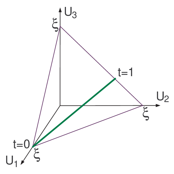
A representative 2-cycle can be constructed as the image of a map which we build as follows. First split the coordinates in two suitable groups by splitting the index set as the disjoint union , with the number of elements in equal to , the number of ’s. Then we put
| (5.17) |
where we choose the path such that the following conditions are met:
| (5.18) |
The first constraint enforces the to satisfy the D-flatness constraints defining , while the two last conditions are needed to make the boundary circles collapse to a point up to gauge transformation, so the 2-cycle is closed in . An example for is plotted in fig. 11.
Then we have for :
| (5.19) |
Similarly, after doing the proper gauge transformation , we find for . This establishes (5.15).
This gives a direct connection between the FI parameters and the Kähler moduli of .
In general the 2-cycles or integer linear combinations thereof will not be holomorphic; the corresponding homology classes might not even have any holomorphic representatives at all. To construct holomorphic curves, one can simply take transversal intersections of of the divisors . By taking positive linear combinations, these in fact generate the full set of all 2-cycle classes with holomorphic representatives (this set is called the Mori cone). The relation with the can be deduced by comparing the intersection products and .
For example for , we have , because indeed . For the -twisted bundle over defined by (5.4), we have
| (5.21) |
so and are holomorphic curve classes, and moreover since and , they generate (with positive coefficients) the full Mori cone of holomorphic curve classes. (Had we chosen , then the Mori cone would be generated by and .)
Finally, since for holomorphic curves the period equals the area of , we must have for all generators of the Mori cone. This translates to a set of inequalities on the . The space of all satisfying for all in the Mori cone is called the Kähler cone. This corresponds to all possible Kähler classes which can be obtained by varying the without degenerating the space . The space of these deformations is called the Kähler moduli space.
One can choose the generators of the gauge group to be such that the are generators of the Mori cone. If this is a complete set of generators, then the Kähler cone is given simply by , and if we then choose a basis of divisors dual to the (i.e. ), we can parametrize the Kähler form as
| (5.22) |
If there are more than generators of the Mori cone, there will be additional inequality constraints on the . Intersection products of the are always positive.
For , we have and with . For our -twisted bundle over , we have , , and with .
At the boundary of the Kähler cone, a 2-cycle collapses to zero area. By keeping on varying the (so formally the curve area becomes negative), one often simply continues to a different smooth geometry in this way, still described by (5.2), but with different intersection products , and with its own Kähler cone. This is called a flop transition, with the collapsing curve being flopped. In other cases, there is no transition to a new smooth geometry, although in the full gauged linear sigma model, the physics remains sensible.
5.4 Volumes
Using the parametrization of (5.22)2424 24 One can of course also consider more general parametrizations with some basis of divisor classes; the resulting expressions are completely analogous. and the intersection products of the divisors, it is straightforward to compute the volume of :
| (5.23) |
Explicitly, for say , parametrizing , this is, using :
| (5.24) |
and for the fibration over , parametrizing , using (5.11)-(5.14):
| (5.25) |
The volume of other holomorphic cycles can be computed similarly. In particular the volume of the divisor is
| (5.26) |
and all other holomorphic divisor volumes can be computed from this by linearity: . Holomorphic intersections are also easy to compute:
| (5.27) |
As an example, the volume of in is
| (5.28) |
In the bundle example, we get
| (5.29) | |||||
| (5.30) | |||||
| (5.31) |
More general volumes can be computed easily as well; for example the formal area of the self-intersection of is
| (5.32) |
Note that this is negative. This simply indicates that the self-intersection of does not have a holomorphic representative. (In general only transversal intersections of holomorphic objects are again holomorphic.) Finally note that in this example, we have
| (5.33) |
Recalling section 4.7, this suggests that these manifolds (as base manifolds of elliptically fibered CY fourfolds) might provide examples of the “Swiss cheese” scenario of section 4.7. We will see in section 7 that this is indeed the case.
5.5 Characteristic classes
Characteristic classes play an important role in string theory in extracting, from geometrical setups, various physical topological quantities such as RR charges, moduli space and flux lattice dimensions, numbers of fermionic zero modes of instantons, and so on. In the following we will first list the general (smooth differential geometric) definitions of the various characteristic classes that appear in this paper, and then specialize to computations of tangent bundle characteristic classes of toric varieties and algebraic submanifolds thereof.
The total Chern class of a rank holomorphic vector bundle with matrix curvature form is defined as the cohomology class of
| (5.34) |
From the properties of the determinant, it immediately follows that . More generally, if we have three vector bundles , , such that (so locally ), then we have the Whitney sum formula:
| (5.35) |
An important example is given by the tangent and normal bundles of a holomorphic submanifold of a manifold . Because the normal bundle of is the quotient of the tangent bundle of restricted to by the tangent bundle of , we have
| (5.36) |
which can be used to compute from knowledge of and . (If for example is given as the intersection of divisors, , then we simply have ). When specifically applied to the tangent and normal bundles of a manifold as just shown here, the Whitney sum formula is usually referred to as the adjunction formula.
In terms of the eigenvalues , , of , we can also write
| (5.37) |
Thus the can be thought of as the formal roots of the total Chern class, and for that reason are called the Chern roots. They are very useful to define and relate various characteristic classes. The Whitney sum formula given above can be thought of as simply splitting the Chern roots of into Chern roots of and Chern roots of .
The Euler class of a holomorphic vector bundle is its top Chern class:
| (5.38) |
In particular the Euler characteristic of a complex manifold equals the integrated Euler class of its holomorphic tangent bundle:
| (5.39) |
Similarly one defines the Chern character as
| (5.40) |
and this satisfies the sum and product formulas and . The Todd class is given by
| (5.41) |
and is multiplicative, like the Chern class. Finally, the Hirzebruch L-genus is
| (5.42) |
and the A-roof genus is
| (5.43) |
The Chern class of a toric variety is given by the particularly simple expression
| (5.44) |
where should be read in the last expression as the Poincaré dual to the divisor in . More generally we get formulas for all characteristic classes defined above by the substitutions , and
| (5.45) |
For example for we have, after using the relations between the toric divisors, and putting :
| (5.46) |
, and . For weighted projective space , defining by , we have
| (5.47) |
For the -twisted bundle over , we get
| (5.48) |
so , , and .
It is also straightforward to compute Chern classes of algebraic submanifolds of toric varieties, by making use of the adjunction formula (5.36). For a submanifold of defined by
| (5.49) |
where the are hypersurfaces given by polynomial equations in the , this yields
| (5.50) |
Similar formulas hold for the other multiplicative characteristic classes. It is important to remember however that these formulas can only be directly applied when the complete intersection is smooth.
As a classic example, consider the quintic hypersurface in :
| (5.51) |
Then, putting ,
| (5.52) |
Note that the first Chern class vanishes: the quintic is a Calabi-Yau manifold. Furthermore
| (5.53) |
5.6 Holomorphic forms and Poincaré residues
Periods of holomorphic forms play an important role in the computation of super- and Kähler potentials. An elegant and useful general construction of such forms is as a Poincré residue, as we now explain.
Any gauge invariant meromorphic form on
| (5.54) |
where is a homogeneous rational function of the , descends to a well-defined meromorphic -form (more precisely a form) on the -dimensional toric variety . The reduction goes as follows. Let
| (5.55) |
be the holomorphic vector fields generating the gauge symmetries (i.e. ). Then the contraction of with all vector fields,
| (5.56) |
is a globally defined meromorphic -form on . If is a polynomial, then is holomorphic.
As a first example, consider . To make gauge invariant, must have charge , so cannot be polynomial and we do not get any holomorphic 2-forms on , but e.g. will do, leading to the meromorphic 2-form
| (5.57) |
For the weighted projective space , must have charge . So in particular when , there are holomorphic 3-forms on , and when , there is a unique one up to overall scale, namely a constant:
Indeed when , the first Chern class is trivial, , so is a Calabi-Yau 3-fold and has a unique holomorphic 3-form. Note however that it is noncompact. (In fact there are no compact toric Calabi-Yau manifolds.)
It is clear that the above construction will always give a unique holomorphic -form when vanishes.
There is also a natural way to construct meromorphic -forms on -dimensional algebraic subspaces of defined by a system of homogenous polynomial equations. Consider first the case of a hypersurface given by . Let again be as in (5.54), but now we take the charges of such that is gauge invariant instead of . Then
| (5.58) |
where the contour is taken to be an infinitesimal loop around , defines a globally well defined meromorphic top form on . The contour integral picks up the so-called Poincaré residue. This can be defined more precisely as follows. Let be a meromorphic -form in an -dimensional space with a single pole along a a smooth hypersurface , locally described by the equation . Near write
| (5.59) |
where and are locally defined holomorphic -forms. Then the Poincaré residue of is the restriction of to :
| (5.60) |
which is unique and extends globally on .
For a space given by a complete intersection of divisors given by the polynomial equations in a toric variety, we can generalize (5.58) by picking to be such that is gauge invariant, and putting
| (5.61) |
Again when vanishes, so is Calabi-Yau, this gives rise to a unique holomorphic top form on .
As an example consider the quintic hypersurface in , defined by a degree 5 homogeneous polynomial equation . On it we have the unique holomorphic 3-form
| (5.62) |
which in a patch where we gauge fix say can be evaluated as
| (5.63) |
Although explicit patch-dependent expressions like this one are often easily computed, the gauge invariant integral form of the residue, like (5.62), is often more useful to compute periods and differential equations satisfied by them. For techniques to explicitly compute periods, see e.g. [110].
Another application of the Poincaré residue is the one to one map between holomorphic deformations of a divisor in a Calabi-Yau -fold and holomorphic -forms on . For a deformation of the polynomial , the corresponding -form is
| (5.64) |
where is the holomorphic -form on the CY. Indeed the number of deformations of a holomorphic divisor in a Calabi-Yau is .
5.7 Calabi-Yau submanifolds of toric varieties
Complete intersections in toric varieties with vanishing first Chern class,
| (5.65) |
provide a large, concrete set of examples of Calabi-Yau manifolds which can be used as target manifolds for string, M or F theory. These manifolds inherit their Kähler moduli spaces from the ambient toric variety, and their complex structure moduli spaces can be identified with the deformations of the defining polynomials modulo coordinate redefinitions.2525 25 In some cases, there may be additional complex structure deformations which do not correspond to defining polynomial deformations.
We consider some examples.
The most general quintic submanifold of is given by an equation of the form with a homogeneous degree 5 polynomial. Such a polynomial has coefficients. Polynomials which differ only by a coordinate transformations of the are isomorphic, so we have independent complex structure moduli.
We can check our moduli counting by computing the Euler characteristic from the Hodge numbers the counting implies and comparing to (5.53). With 1 Kähler modulus and 101 complex structure moduli, the independent Hodge numbers of are , , so the independent Betti numbers are , , and , and , in agreement with (5.53).
The quintic inherits a Kähler class from the Kähler class of , by pulling back to . It is usually convenient to express in terms of a basis of . Such a basis is obtained by intersecting the divisor basis of the ambient variety with the hypersurface. In this case this consists of the single element . Then . The intersection numbers for this basis follow directly from the intersection numbers of the ambient toric variety:
| (5.66) |
A somewhat more complicated example is the Calabi-Yau fourfold elliptically fibered over as considered in section 3.8. To cast this in gauged linear sigma model language, we first define a five complex dimensional toric variety by introducing seven fields , identified with the variables used in section 3.8 as
| (5.67) |
We assign these fields the following charges:
| (5.68) |
And take the corresponding FI parameters and positive. The assignment of the charges is uniquely fixed (up to change of basis of generators) by the Calabi-Yau condition (5.65) and the form of the equation . This also fixes the charges of the polynomials and . We picked a slightly different basis of generators compared to (3.60), to make the associated curves and to form a basis of the Mori cone. The divisors
| (5.69) |
dual to , form a basis for the Kähler cone. Note the relations
| (5.70) |
Using the techniques described in section 5.2, we find the intersection products
| (5.71) |
There is a quotient singularity at , and a quotient singularity at , , explaining the fractional intersection numbers. For example the third intersection number is obtained by noting that , and that the intersection between those five distinct divisors is given by an up to gauge transformations unique, regular point .
The elliptically fibered Calabi-Yau itself is given by (3.59):
| (5.72) |
This hypersurface avoids the quotient singularities of the ambient toric variety: for example if , then (5.72) implies , but the point is excluded by the D-term constraints. The homology class of is
| (5.73) |
and the intersection products of the pullbacks are, by the rule :
| (5.74) |
Note in particular that
| (5.75) |
The Kähler class on is with , and hence the volume of is
| (5.76) |
A representative elliptic fiber of is given by , so its homology class in is . Hence the area of the elliptic fiber is
| (5.77) |
This is exactly the parameter introduced in section 3.1. A section of the base of the fibration is given by , so its homology class is , and its volume
| (5.78) |
In the F-theory limit on M-theory, we send . In this case
| (5.79) |
as expected from the explicit form of the metric (3.18) in this limit.
The total Chern class of the fourfold is, using (5.50) and (5.70) and the intersection numbers:
| (5.80) | |||||
We repeatedly used , and denotes the unit volume element on . In particular we thus read off the Euler characteristic of the fourfold:
| (5.82) |
Hence for this example, the number appearing in the tadpole cancelation condition (4.97), i.e. minus the curvature induced D3-charge, equals .
5.8 Index formulae
To count various massless string modes (i.e. bosonic and fermionic zero modes), it is very useful to have index formulae relating various indices to expressions involving characteristic classes.
For a -form we define the fermion parity . The simplest index is
| (5.83) |
where and is the Euler class defined in (5.38).
Twisting this index by the Hodge star operator gives:
| (5.84) |
Here is the complex dimension of , is the number of (anti-)selfdual harmonic -forms on , is called the signature of , and is the Hirzebruch -genus of the tangent bundle of as defined in (5.42). This is the Hirzebruch signature formula.
On Kähler manifolds there are holomorphic versions of these index theorems, which sum over (bundle valued) -forms only. These are typically relevant to count brane moduli or fermionic zeromodes. The simplest is the arithmetic genus / holomorphic Euler characteristic formula
| (5.85) |
where the Todd class was defined in (5.41). This formula will allow us to check whether M5 instantons satisfy the necessary condition (4.90) to contribute to the superpotential.
This can be generalized to bundle-valued forms:
| (5.86) |
This is the Hirzebruch-Riemann-Roch theorem.
5.9 Computing Hodge numbers
Hodge numbers , or at least a set of relations between them, can be computed using the above index theorems.
In particular, from (5.86), taking , i.e. the space of -forms on , and using , we get a formula for the arithmetic genera :
| (5.87) |
can be computed as follows. First note that is just the holomorphic cotangent bundle , which is dual to the tangent bundle , so in terms of Chern roots, if , we have , and . Now , i.e. the antisymmetrization of . More physically, one can think of this as the space of 2 particle states built from the 1-particle fermionic states of , where the one particle states have curvature eigenvalues . It follows that the 2-particle states have eigenvalues , , so . This reasoning can be continued to higher ; an efficient way to summarize the result is by the fermionic generating function:
| (5.88) |
Combining this with (5.87) and (5.41), we obtain the generating function for all arithmetic genera
| (5.89) |
known as the Hirzebruch genus.
This allows us to read off the following results. For :
| (5.90) | |||||
| (5.91) |
These expressions can be used to determine and once is known. For :
| (5.92) | |||||
| (5.93) |
Note that the formula for allows us to rephrase the necessary condition (4.90) for M5 instantons to contribute to the superpotential as . Furthermore for subspaces of toric varieties, the formula (5.50) allows to explicitly compute this.
Finally, applied to Calabi-Yau fourfolds (so ):
| (5.94) | |||||
| (5.95) | |||||
| (5.96) |
For Calabi-Yau fourfolds we also have (and of course ) and if the holonomy is full , then . The equations then becomes trivial, and the and equations can be used to determine and in terms of and , i.e. the number of Kähler and complex structure moduli.
For the fourfold example (3.59) discussed above, we have Kähler moduli and complex structure moduli (obtained by direct counting of the number of polynomial deformations modulo reparametrizations). Furthermore, using the above expressions together with (5.80), we get
| (5.97) |
This determines
| (5.98) |
As we see illustrated in this example, we still need the number of complex structure moduli (or alternatively some other Hodge number such as ) as input. In the case at hand we obtained the correct result by counting polynomial deformations modulo coordinate redefinitions. The problem is that sometimes there are complex structure deformations which are not given by polynomial deformations. In this case, more sophisticated techniques are needed; see e.g. [55] for CY fourfolds in particular.
6 Statistics of flux vacua
We need one last ingredient before we can start our search for explicit realizations of the moduli stabilization scenarios of sections 4.6 and 4.7: efficient estimates of distributions of tree level flux vacua over parameter space. This is necessary because constructing fully explicit flux vacua in typical F-theory compactifications would require specifying 20,000 or so flux quanta and finding the corresponding critical points in the 3000 or so dimensional complex structure moduli space, hoping to hit the region of parameter space we are interested in (e.g. weak string coupling, tiny cosmological constant, …) — an effectively intractable task.
The statistical approach to flux vacua was initiated in [111] building on ideas of [104], and further developed in [101, 28, 112] and subsequent works. An extensive review can be found in [26], and a more pedagogical review in [113].
6.1 The Bousso-Polchinski model
It was pointed out in [104] that the freedom one has to turn on various independent flux quanta in string theory compactifications can lead to huge ensembles of vacua with a “discretuum” of low energy effective parameters; like the continuum, the discretuum allows for fine tuning, but without the massless moduli necessarily associated to continuously variable parameters.
This is true in particular for the cosmological constant, implying naturally the existence of string vacua with exceedingly small effective four dimensional cosmological constants, such as our own, without the need to invoke any (so far elusive) dynamical mechanism to almost-cancel the vacuum energy.
To see how this comes about, consider the potential induced by some flux characterized by flux quanta , , of the general form we considered in section 2:
| (6.1) |
where denotes the moduli of the compactification manifold and is some positive definite effective metric on the moduli space. Further on we will be interested mainly in F-theory flux vacua, but at this point we just consider the above potential as an abstract starting point for a toy model. In particular we ignore constraints such as tadpole cancelation conditions. The bare potential is taken to be negative. In the context of string theory, it will be of the order of some typically high fundamental scale, such as the string or KK scale.

Each vacuum of this model is characterized by a choice of flux vector together with a minimum of . As a further drastic simplification however, let us, following [104], simply freeze the moduli by hand at some fixed value and ignore their dynamics altogether. In that case becomes just a quadratic function of , and it is then easy to compute the distribution of cosmological constant values. The number of vacua with cosmological constant less than is now simply given by the number of flux lattice points in a sphere of radius squared , measured in the metric. When is sufficiently large, this is well-estimated by the volume of this -dimensional ball, i.e.
| (6.2) |
This leads to the following vacuum number density as a function of :
| (6.3) | |||||
| (6.4) |
where can be interpreted as the typical mass scale of the flux part of the potential. To get the last approximate expression, we assumed large and used Stirling’s formula. Note that in particular at , for say , we get a vacuum density . Hence for a few hundred, there will be exponentially many vacua with in the observed range , even if all fundamental scales setting the parameters of the potential are of order !
Thus, in such a model, there is no need to postulate either anomalously large or small numbers, or an unknown dynamical mechanism, to obtain vacua with a small cosmological constant.
However, explicitly finding the flux vectors which give rise to such a small cosmological constant is, even this extremely simplified setting, in general an effectively intractable problem: suitably formalized, this inversion problem can be proven to be NP-hard [114]!
6.2 Distributions of F-theory flux vacua over complex structure moduli space

6.2.1 Setting up the counting problem
We now turn to the problem of counting genuine F-theory flux vacua and computing their distributions over complex structure moduli space. As we have seen in section 4.4.3, a (tree level) F-theory flux vacuum on an elliptically fibered Calaby-Yau fourfold is characterized by
- 1.
A choice of flux quanta , determining the flux by , satisfying the tadpole cancelation condition (4.97)
(6.5) If we require , this imposes the bound
(6.6) - 2.
A critical point in complex structure moduli space of the superpotential
(6.7) where , with being the Kähler potential.
The number of zeros of a function of one real variable is
| (6.8) |
Similarly, the number of flux vacua in a given region of complex structure moduli space is
| (6.9) |
where is the complex dimension of the complex structure moduli space and the sum is over all fluxes satisfying (6.6). The determinant factor ensures that each zero of contributes to the integral, analogous to the factor in (6.8). In vacua for which , there will be residual D3 moduli at tree level. They may however be lifted after inclusion of quantum effects. This will give an additional contribution to the vacuum degeneracy, not taken into account in (6.9). Similarly, the Kähler sector, left completely unfixed at tree level, may after inclusion of quantum effects give an additional vacuum degeneracy, or even destabilize the compactification altogether. At this stage however, we wish to focus exclusively on the tree level flux and complex structure sector, so (6.9) is adequate.
Note that the number of vacua without any D3-branes is just
| (6.10) |
Of course (6.9) is not terribly useful yet. To make further progress, we will need to make some approximations. First, we will approximate the sum over fluxes by an integral. This is the analog of computing the number of lattice points in the Bousso-Polchinski sphere by computing its volume, and can be expected to be a good approximation in the large limit. Second, we will drop the absolute value signs around the determinant factor in (6.9). This means we will be counting vacua with signs depending on the number of positive and negative eigenvalues of ; in other words we are computing some sort of index. Strictly speaking this will only give a lower bound on the number of vacua, but in practice the index can be expected to give a good estimate of the order of magnitude of the actual number of vacua in the given region, since there is generically no particular reason for large cancelations.
Before we proceed, we will prove a counting formula in abstract generality which can be applied to many different instances of counting of flux vacua.
6.2.2 A general asymptotic counting formula for zeros of vector field ensembles
Consider a region in a space with real2626 26 We switch to real variables here because this makes notation more compact and because it gives a more general formula. coordinates , . Let , be a set of real vector fields, and let be a nondegenerate symmetric matrix with inverse . For a choice of integral “flux quanta” satisfying the constraint
| (6.11) |
we define
| (6.12) |
In applications to counting actual flux vacua, this vector field will essentially be the gradient of the superpotential. The set of “flux vacua” we wish to count are labeled by with
| (6.13) |
Hence, similar to (6.9), we wish to estimate
| (6.14) |
where the sum is restricted to (6.11). We will approximate this by the continuum index
| (6.15) |
This can be evaluated as follows. Define a metric on by
| (6.16) |
We assume that is nondegenerate on . We also define a covariant derivative such that
| (6.17) |
i.e. with
| (6.18) |
Then we claim
| (6.19) |
where is the Euler density derived from the connection :
| (6.20) |
with is the Pfaffian and the curvature form in an orthonormal frame with respect to (underlined indices are frame indices):
| (6.21) |
The proof goes as follows. We define a generating function
| (6.22) |
where now the integral over is unrestricted. Trading partial derivatives for covariant derivatives in (6.15) or vice versa here does not affect the result, because the difference between and vanishes when . The index (6.15) at given is obtained from the generating function by the contour integral
| (6.23) |
where the contour runs over the imaginary axis passing the pole on the left. (Then if , we close the contour on the right and we pick up 1 from the pole, while if we close the contour on the left and the result vanishes. This enforces the constraint (6.11).)
Furthermore we write
| (6.24) | |||||
| (6.25) |
where the second integral is over Grassmann variables. Substituting this, the integral over in (6.22) becomes a simple Gaussian integral,2727 27 In general need not be positive or negative definite, in which case the Gaussian integral is defined by analytic continuation. resulting in
| (6.26) |
where
| (6.27) |
Now note that because of (6.17), the - cross terms obtained when expanding out all vanish. The remaining terms are proportional to
| (6.28) | |||||
| (6.29) | |||||
Performing the Gaussian integrals over and , then gives, using the Grassmann integral representation of the Pfaffian:
| (6.30) |
with the Euler density defined in (6.20). Extracting from the contour integral (6.23) finally gives
| (6.31) |
as claimed.
The prefactor can morally be thought of as giving the volume of a sphere of radius in flux space. (This is exact when is positive definite; if not, it is a volume in an analytically continued sense).
If is taken to be a compact, closed manifold and is sufficiently well-behaved, then the integral of the Euler density is a topological quantity, the Euler characteristic of the bundle for which is a connection. For example when the are ordinary sections of , then , the Euler characteristic of . In this case, our counting formula reproduces the well known fact that the number of zeros of a vector field on a compact closed manifold, counted with signs, equals the Euler characteristic. However, for our formula, we actually only need the ensemble of vector fields to be single valued; there may be monodromies acting on the individual vector fields (as will be the case typically for F-theory flux vacua). Furthermore, can be any region, and we do not just get the total number of zeros, but their actual distribution as a particular density function .
One interesting general feature following from the expression (6.31) is that flux vacua will tend to cluster anomalously in singular regions where diverges. We will confirm this below for the example of flux vacua near conifold degenerations, where strong warping occurs.
6.2.3 Application to F-theory flux vacua
Although we derived (6.19 thinking of the , as real variables, we could have thought of them as complex variables , as well, by formally setting for and for and similarly for and for . Everything else would still have gone through, and in particular (6.19) remains true. In case happens to be a hermitian metric, i.e. , the Euler class can also be written in terms of a determinant, as usual for complex varieties with a hermitian metric.
With this in mind, we can immediately apply our result to counting F-theory flux vacua , taking to be a region in complex structure moduli space and
| (6.32) |
where the are the fourfold periods as in section 6.2.1. Furthermore we take , with the intersection product (6.5).
With these choices, the metric (6.16) has components
| (6.33) |
The first equation holds because of Griffiths transversality: The derivative of a -form with respect to the complex structure moduli produces a form of type . Hence and therefore is of type . (In fact the covariant derivative is defined in precisely such way that is exactly of type .) In any case the wedge product of forms is zero, implying . The second equation is a consequence of the same Griffiths transversality and the definition of .
Thus, interestingly, we find that the auxiliary metric (6.16) in this case exactly coincides with the physical metric on complex structure moduli space, which appears in the low energy effective action.
As for the covariant derivative , this is defined in (6.17) by requiring
| (6.34) |
where . Again using Griffiths transversality, it can easily be shown that this is satisfied for the standard Levi-Civita and Kähler covariant connection [28] on with the Kähler line bundle of which the supergravity superpotential is a section:
| (6.35) | |||||
| (6.36) |
Here is the Levi-Civita connection of .
Hence we conclude that the continuum index of F-theory flux vacua satisfying (6.6) is
| (6.37) |
where the euler density of can be written, using the fact that we have a complex structure, as
| (6.38) |
Here is the curvature form of the holomorphic tangent bundle to and is the Kähler form on , which is the curvature form of .
The F-theory flux lattice dimension is given by , where is the number of 4-form fluxes with one leg on the elliptic fiber; more formally, it is the dimension of the subspace of orthogonal to intersections of divisors, i.e. satisfying (4.44). For the fourfold example (3.59), we read off from (5.98) that , while (4.44), taking into account the relation (5.75), imposes two independent constraints. Therefore . Furthermore, as we saw below (5.82), . The intersection form on the full lattice , as on any middle cohomology lattice on a compact manifold, is unimodular, i.e. has determinant 1. The sublattice of divisor intersections can be seen to be unimodular too using the results of (5.74), and the orthogonal complement of a unimodular lattice is unimodular. Therefore , and
| (6.39) |
If we let be the entire complex structure moduli space, then the integral equals the Euler characteristic of .2828 28 Actually since the moduli space has singularities, the notion of Euler characteristic is ambiguous, and in particular the integral of the above Euler density need not coincide with the topological Euler characteristic. We assume it nevertheless coincides with at least one of the several natural notions of Euler characteristic for singular varieties. Since the moduli space is some simple quotient of a projective space (namely the space of coefficients of the defining polynomial modulo coordinate redefinitions), one expects this number to be essentially order 1 compared to the exponential prefactor.
The continuum index of vacua with is, analogous to (6.10):
| (6.40) |
In fact, when the number of vacua is exponentially large, almost all flux vacua have according to this estimate; this is related to the fact that for a high dimensional sphere, almost all enclosed volume is located very near its boundary. For our example:
| (6.41) |
This illustrates we have to be particularly careful not to naively apply our low dimensional intuition to high dimensional situations.
We will discuss to what extent the continuum index does (not) give a good estimate for the actual number of vacua, counted with or without signs, in section 6.3.
A final comment is in order. For a small domain , can be quite precisely thought of as the volume in flux space of the set of which give rise to a solution of located in . Given the somewhat formal nature of the general computation of , in particular the use of analytic continuation in evaluating the Gaussian integral , one may worry if the result we find does correctly represent this volume in flux space. In particular, given the fact that is not positive or negative definite, one might worry that the actual volume is in fact infinite. However, the condition effectively renders positive definite, since as we saw in section 4.4.3, implies , and therefore . Hence for any finite region away from singularities, will indeed be finite. Finiteness near singularities and of the actual number of IIB flux vacua has been analyzed in [101, 115, 116]. In [13] the question of finiteness of string vacua was addressed in a much more general setting, and it was argued that, remarkably, in regimes which are in principle under control, the total number is finite as long as one stays bounded away from decompactification limits (characterized by KK modes becoming light).
6.2.4 Application to IIB bulk flux vacua
Most of the statistical analysis in the literature has been done purely in simplified models in which one only considers the IIB bulk sector, neglecting D7 degrees of freedom. One can effectively think of these simplified models as F-theory on with some Calabi-Yau 3-fold. Note that taken literally, these models have zero Euler characteristic, so and no flux vacua. However, we can still formally count solutions to , by choosing some by hand. The number of effective F-theory fluxes is now
| (6.42) |
namely RR fluxes ( leg on -cycle ) and NSNS fluxes ( leg on -cycle ). The intersection form is obtained from the symplectic intersection forms on and , and again unimodular. With these substitutions, all of the above formulae remain valid. These simplified models are presumed to give estimates in some sense for the number of bulk flux vacua in the weak IIB coupling limit, although this has not been made precise. From our considerations in section 4.4.4, it seems plausible that this makes sense if all D7 branes are coincident with the O7-planes, although turning on bulk NSNS fluxes generically does not appear to keep the D7-branes there.
Taking to be the Calabi-Yau 3-fold arising in the weak coupling limit of the model (3.59), we get , and therefore the continuum index for a region of the bulk moduli space (complex structures of and ), putting , is
| (6.43) |
The restriction to these simplified models is why is such an infamous number, rather than one of the much bigger numbers one gets out of the full F-theory estimates.
6.2.5 Toy model

As a simple illustration, consider again the toy model introduced at the end of section 4.2 and further analyzed at the end of section 4.4.3. As we saw there, the critical points can be computed exactly, and all inequivalent flux vacua for a given can be systematically enumerated [101]. The exact vacua for are plotted in fig. 14. The continuum index distribution is also straightforwardly obtained [101, 28]. The Euler density is
| (6.44) |
hence
| (6.45) |
where is the area of the region under consideration in the Kähler metric (4.15). Letting be the entire fundamental domain, we get .
Despite the intricate fine structure as evident from figure 14 (in particular the striking “voids” around simple complex rational numbers), it is nevertheless true that for large a disc of sufficiently large area will contain approximately vacua. This is illustrated for in figure 15, where estimated and real numbers of vacua are compared in discs around the center of the largest hole of stepwise increasing radius.
In more complicated models there are many more fluxes and the periods are highly complex functions. As a result, flux vacua will be much more randomized than in this simple example, and continuum distributions can be expected to become good approximations already at finer scales. Some more comparisons between exact and approximate distributions can be found in [66].

6.3 Regime of validity and improved estimates
We now turn to the question when the continuum index is a good approximation for the actual number of vacua, or at least the actual discrete index of vacua. On general grounds we expect the continuum approximation to be valid in the large limit, but since is given to us by the topology of , we need to understand better what qualifies as “large”.
To get an idea when the approximation certainly fails, we approximate the prefactor of (6.37) using Stirling’s formula (and assuming ) as
| (6.46) |
When , this is in fact exponentially small! This is related to the fact that the volume of a sphere of fixed radius goes to zero exponentially when the dimension is sent to infinity. Clearly, in this regime, the approximation breaks down badly. The reason is that in this regime a large fraction of the flux quanta will be zero or some small integer, so the continuum approximation is no longer valid.
In general we have and , so in models with (as is the case for our example and in the models listed in appendix B.4 of [55]), we have . Then
| (6.47) |
so we are barely above the threshold where things go wrong badly. This indicates the continuum index may be a serious underestimate of the actual number of flux vacua in F-theory.

To make this more precise, let us consider as a toy model the problem of counting the number of lattice points in a sphere of radius . In the large limit, this is the volume of the sphere:
| (6.48) |
The exact number can be represented as
| (6.49) |
with , and where we take the contour along the imaginary axis, passing the pole on the left (compare to (6.23)). For large , the integral can be computed by saddle point evaluation:
| (6.50) |
The results relevant for our usual example are shown in fig. 16. We see that the continuum approximation becomes very good when becomes larger than about , but that in the regime of interest , the approximation is poor.2929 29 In the simplified bulk flux models introduced in 6.2.4, which have been the main focus in the literature, this problem typically does not arise, because the number of IIB bulk fluxes is usually much smaller than the total number of F-theory fluxes. In our example, the number of bulk fluxes is , so is well above , and the continuum approximation is excellent.
In fact when and is large, we find and
| (6.51) |
The continuum estimate on the other hand gives . For our example , so while the continuum estimate gives a measly .
A natural guess for an improved estimate of the number of F-theory flux vacua would be to replace the volume factor in (6.37) by our toy model
| (6.52) |
However, one should worry that the sparseness of the typical flux vector in the ensemble will have significant effects on the distribution density as well, drastically modifying the density valid in the continuum approximation. In particular, one could imagine discrete effects such as clustering at enhanced symmetry loci to become more important. This has not been studied yet.
Note that as a rule of thumb, this estimate amounts to about a factor of 10 per moduli space dimension.
6.4 More distributions
6.4.1 Distribution of
So far we have only discussed estimates for the total number of flux vacua and their distribution over complex structure moduli space. It is not hard to extend this to distributions of other quantities, such as the distribution over the plane. To estimate the latter in the continuum index approximation, one can insert an additional in the generating function for , rewrite this using Lagrange multipliers, integrate out and use Griffiths transversality again, to find that the net effect of this additional insertion is (up to some constant factor) . So effectively, this amounts to replacing and , and we find for the combined distribution
| (6.53) |
where is the usual sphere volume factor in the continuum approximation, or the function introduced in the previous subsection in cases where we believe this to be a better estimate. Note that at large , due to the exponential dependence of on , this distribution is approximately Gaussian on the -plane, peaking at and cut off at . This is as one would expect if one thinks of as being the result of a random addition of a large number of complex numbers. The cutoff can be understood as well, it comes from , where we used that .
The width of the Gaussian is , which in the case of fig. 16 is somewhat less than one. For applications in constructions of string vacua we are however mainly interested in vacua with . In this regime, the distribution becomes uniform on the -plane:
| (6.54) |
as can be expected on general grounds. In particular this implies we can expect vacua with roughly as small as .
6.4.2 Distribution of string coupling constants
From the considerations in section 4.3, we know that in Sen’s weak IIB coupling limit, the fourfold complex structure moduli space factorizes in a dilaton-axion moduli space, a threefold complex structure moduli space, and (depending on the point in the threefold complex structure moduli space), a D7 moduli space. Hence we get a corresponding factorization of the continuum index density
| (6.55) |
where is some -independent density on the threefold complex and D7 moduli spaces, while is the Kähler form on the dilaton-axion moduli space (which proportional to the curvature form), i.e.
| (6.56) |
as in (6.44).
This implies in particular that universally in the weak coupling limit (i.e. sufficiently large), is uniformly distributed w.r.t. the standard Poincaré metric on the upper half plane. In terms of the string coupling constant , this is simply the uniform distribution:
| (6.57) |
The continuum approximation for the distribution is expected to be accurate down to , where “void” effects like in the toy model might start to get important. (For example in the toy model the actual minimal value of is , although the continuum approximation predicts an order minimum; the discrepancy can be thought of as being due to the void around .)
6.4.3 Conifold clustering and distribution of warp factors
Consider a simplified bulk flux model as described in section 6.2.4, with a one modulus Calabi-Yau threefold. An example is the mirror quintic, described by
| (6.58) |
in , modulo phase transformations leaving this equation invariant. acquires a conifold singularity when . Parametrizing , the distribution near in the continuum approximation can be computed from (6.38) to be [28]
| (6.59) |
The distribution diverges at , but in an integrable way, and is approximately scale invariant. As a result, there will be a sizable number of flux vacua exponentially close to the conifold point. Now recall from section 4.4.6 that flux vacua close to conifold points develop a strongly warped KS-type throat. The redshift at the bottom of the throat is given by (4.75): , so the above distribution can be viewed as a distribution for warp factors. In the case of the mirror quintic, this gives, taking into account numerical factors and setting , about 3% of all flux vacua has , 0.7 % has , and 0.3 % has .
Similar to the string coupling constant, one expects the continuum distribution to be accurate for roughly down to .
Having 0.3% of flux vacua with warping may not sound like a terribly spectacular enhancement. Admittedly, it isn’t. However in generic actual models, there are many more 3-cycles which could potentially shrink to a tiny size, and this may lead to a much higher fraction of vacua with one or more warped throats, as the following simple argument shows. Imagine we have a Calabi-Yau threefold with 3-cycles which could potentially collapse to zero size. Then the mirror quintic data suggests that a naive rough estimate for the fraction of vacua for which all of these 3-cycles remain larger than the size to get is equal to something like . Now when becomes large, this can become a small fraction. For example if , about half of all vacua do have , and if , this goes up to 80%. Of course the actual numbers we used here are just for illustration purposes; but the general idea should be clear. This was studied in more detail in [117].
The above simple argument relies on many poorly justified assumptions though, and is therefore not conclusive. No concrete model has been studied in which these ideas have been tested against actual distributions.
6.4.4 Distribution of compactification scales
In the KKLT scenario of moduli stabilization, the compactification radius is determined by the value of :
| (6.60) |
Therefore, from (6.54), in this scenario, the KK scale is distributed as
| (6.61) |
That is, large volumes are exponentially suppressed, with maximal values of order .
6.4.5 Distributions of nonsupersymmetric flux vacua
The flux vacua we have been considering so far are generically nonsupersymmetric at tree level, with supersymmetry breaking scale , due to the fact that . However in for example the KKLT scenario, supersymmetry gets restored by -dependent quantum corrections. There could be other minima of the full effective potential where supersymmetry is still broken, by some generic . Note that at tree level is forbidden by the equations of motion, so in order to get such minima, the full quantum corrected effective potential must be considered. This is in general a complicated problem.
A slightly simplified model is to consider again the flux superpotential and the supergravity potential , but now without including any contributions from the Kähler moduli — in fact pretending there are no Kähler moduli whatsoever in the game. In particular solutions to will now have negative , because the covariant derivatives with respect to the Kähler moduli are no longer there and so no longer kill off the term.
By “nonsupersymmetric flux vacua” we mean in this model the minima of which have . We are interested in the regime , that is supersymmetry breaking well below the fundamental scale. Then it was shown in [112], and more intuitively explained in [118], that for generic flux vacua the distribution of supersymmetry breaking scales and cosmological constants goes as
| (6.64) |
This “favors” high scale supersymmetry breaking. In [118] the possiblity was considered that other branches of the landscape could exist where low scale breaking was favored. The issue whether string theory favors high or low susy breaking remains inconclusive, and will remain so as long as we have no clue what “favored” means.
6.5 Metastability, landscape population and probabilities
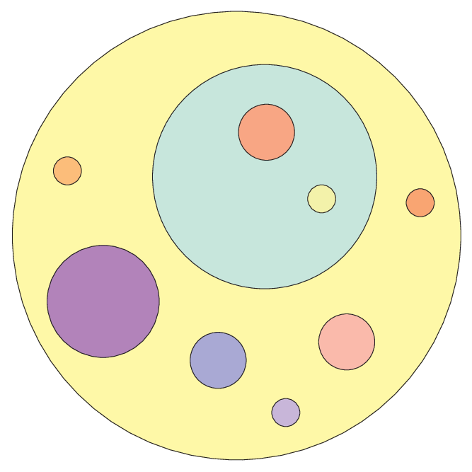
So far we have only considered number distributions of flux vacua over parameter space. It is of course tempting to wonder if there is any sense in which one could, as in statistical mechanics, compute probability distributions on parameter space. This, of course, immediately runs into a heap of conceptual problems. To begin with, it already unclear of what exactly these would be probabilities. At a vague level, one would imagine it to be the probability of finding ourselves in a particular vacuum, but making this precise, given the fact that we already found ourselves here and that there is no way to repeat the experiment, is challenging to say the least.
But regardless of the precise definition of these probabilities, it is clear that to determine them, cosmological considerations will come into play in an important way. In particular, it is necessary to consider the mechanism by which vacua actually come into existence. As we saw in section 3.4, fluxes are sourced by 5-brane domain walls wrapping internal cycles; the flux jumps across such domain walls. Now, if we are in a flux vacuum with positive cosmological constant, quantum fluctuations can cause nucleation of flux-changing domain wall bubbles [119, 120, 104, 121], by a tunneling mechanism similar to Coleman-de Luccia bubble nucleation in scalar potential landscapes. If the cosmological constant inside the bubble is positive again, it will itself inflate and eventually nucleate new bubbles, and so on (see fig. 17 for a psychedelic impression of this). This is a version of eternal inflation (see e.g. [123] for a brief review, and Steve Shenker’s lectures at this school).
Even if we are not interested in computing probabilities, such bubble nucleation processes are still of crucial importance to determine to what extent particular vacua are metastable.
According to [119, 120],3030 30 Their analysis does not take into account moduli dynamics and is intrinsically done in a thin-wall approximation as the membranes are taken to be infinitely thin. The resulting formulas should therefore be taken to be estimates rather than exact results for F-theory flux vacua. the nucleation rate per unit 4d spacetime volume for a bubble with tension , cosmological constant outside and cosmological constant inside is given by
| (6.65) |
where (in units with , which we will use in the remainder of this section):
| (6.66) |
Here and is the bubble radius, which must be evaluated at the stationary3131 31 This is a minimum iff . point of :
| (6.67) |
If , there is always a nonzero nucleation rate. If and the initial space is AdS, one needs in addition and the argument of the square root of (6.67) to be positive (which is automatic if ).
Consistency of the semiclassical approximation requires and therefore exponentially small decay rates, as usual with instantons. In particular any well-controlled domain wall bubble will almost tautologically give rise to an extremely small decay rate. Note that is infinite and the decay rate zero when ; this is the case when the domain wall is BPS saturated, interpolating between two superymmetric vacua.
When with and , this becomes
| (6.68) |
and when :
| (6.69) |
Notice that after restoring powers of , (6.68) does not involve Newton’s constant — the result is indeed identical to the rate of bubble nucleation in the absence of gravity, in the thin wall approximation. The second expression does depend on Newton’s constant. This rate is extremely suppressed for vacua with such as our own (although it is always larger than the Poincaré recurrence rate ). Thus for the stability of a vacua, the most dangerous domain wall bubbles are those with small tension but sizable change of cosmological constant.
Decay rates such as those give here can be taken as starting point to try to find sensible probability measures on the landscape, as explained by Steve Shenker at this school.
7 Explicit realizations of moduli stabilization scenarios
In this section we will finally get to building explicit models of moduli stabilized F-theory flux vacua, drawing on all of the techniques developed in earlier chapters. From the section on statistics, we already take that typically, there will be a fine discretuum of vacua which we can use to tune various physical parameters to our liking, and in particular generate large scale hierarchies through warping. This allows us to consider controlled regimes.
The main remaining challenge is to make sure all Kähler moduli are stabilized. In both the KKLT and the large volume scenarios, this hinges on the existence of suitable nonperturbative corrections to the superpotential. The first concrete models satisfying the necessary geometrical requirements for this (in the KKLT scenario) were proposed in [125], and a simpler and more explicit model was given in [126] and subsequently generalized in [127, 128]. Various powerful mathematical criteria for M5 instantons to have the right zeromode structure to contribute to the superpotential were systematically developed in [124]. We will however stick to the more elementary methods we have developed in these lectures. We will in these lectures also not show explicitly the existence of a Kähler stabilized minimum of the effective potential, but only show that models exist where we do get the necessary structure of the Kähler potential and the right kind of contributions to the superpotential to make in particular the large volume scenario of section 4.7 work. But once these conditions are met, the existence of large volume minima of the effective potential in this scenario is guaranteed by the general analysis of [5, 105, 106, 89]. (However as noted in section 4.7 one should still check if the “small” Kähler moduli in string units can be made sufficiently large to trust the geometrical picture; we will not do this here.)
7.1 The elliptic fibration over
Let us first see if we can turn our basic example (3.59) in an explicit realization of one of the moduli stabilization scenarios outlined in sections 4.6 and 4.7. The large volume scenario needs at least two Kähler moduli, so this is excluded, leaving only the KKLT scenario. To make this scenario work we need some nonperturbative contributions to the superpotential, and the existence of classical flux vacua with exponentially small . As explained in section 6, according to the distribution estimates, there is certainly no shortage of the latter. Generating nonperturbative corrections to is more subtle. As noted in section 4.5.4, in the M-theory picture, all nonperturbative effects can be thought of as being generated by holomorphic M5 instantons wrapping the elliptic fiber and a divisor in the base. A necessary condition for this instanton to contribute in the absence of fluxes is the arithmetic genus condition (4.90). In the presence of fluxes this gets replaced by the weaker condition (4.92): .
In the notation of section 5.7 where we studied this case as an example, the most general holomorphic divisor in wrapping the elliptic fiber is given by some degree polynomial equation on the base, so , . To compute , we use the index formula (5.92): . Here the Chern classes and are those of the tangent bundle of , which can be computed from the Chern classes of the ambient CY fourfold using the adjunction formula (5.36): . But we know already; it is given by (5.80). Expanding out the adjunction formula quotient, we find
| (7.1) |
and from this, using the formula for just quoted and the intersection numbers (5.74):
| (7.2) |
In particular this is always negative, so even the weak condition is not satisfied.
We conclude that neither the large volume, nor the KKLT scenario for this model works.3232 32 Actually, if we tune the complex structure moduli to a locus of enhanced gauge symmetry as discussed in section 3.10, so becomes singular, there could still be nonperturbative contributions associated to M5 instantons wrapping the divisors obtained by blowing up the singularity (i.e. going to the Coulomb branch), as explained in section 4.5.3. The blown up fourfold will have different Hodge numbers than the original , and as a result different flux lattice dimensions and D3 tadpole. Whether we still consider this to be the same model is a matter of semantics. We will consider it to be a different model here.
7.2 The elliptic fibration over
We consider now the CY elliptic fibration with as base manifold our example (5.4), which we denoted by , the bundle over with twist .3333 33 The cases are isomorphic to by exchanging and . This was defined by five fields, which we will now call , and gauge group, with charges
| 1 | 1 | 1 | ||
| 0 | 0 | 0 | 1 | 1 |
and positive FI parameters . Recall from (5.33) that the volume of , is indeed of Swiss cheese type.
We consider again a CY elliptic fibration of the form
| (7.3) |
over , and the Calabi-Yau condition fixes the charges of the fields and polynomials to be
| 1 | 1 | 1 | 0 | 0 | 0 | ||||
|---|---|---|---|---|---|---|---|---|---|
| 0 | 0 | 0 | 1 | 1 | 0 | 0 | 8 | 12 | |
| 0 | 0 | 0 | 0 | 0 | 2 | 3 | 1 | 0 | 0 |
The corresponding D-term constraints are, explicitly:
| (7.4) | |||||
| (7.5) | |||||
| (7.6) |
In accord with the F-theory limit of vanishing elliptic fiber, we take the third FI parameter much smaller than .
It may seem like we have constructed an infinite number of Calabi-Yau fourfolds, labeled by . This is not true. We should keep in mind that we have made the implicit assumption (by using the formula ) that is smooth. If this is not the case, we should in principle first resolve the singularities before applying this formula, or use a modification of the formula appropriate for singular spaces. Now, from the charges of the polynomials and given above, we see that if , and become negatively charged under the first and so must necessarily contain an overall factor equal to a power of . More precisely , where is the smallest integer and the smallest integer . So in this case , and the discriminant vanish as some power of on the divisor , and hence the fourfold is singular along the locus . For not too large, the singularities are harmless in the sense that they can be resolved while preserving the condition, and moreover they have a clean physical interpretation as loci of enhanced gauge symmetry, as mentioned in section 3.10. For example for , we generically have , and , so from the table in section 3.10 we read off that we get an gauge group enhancement. For , we have , , and we get an gauge group enhancement. For , we fall off the table; at this point the singularity becomes so bad that it cannot be resolved preserving the CY condition. This puts a cutoff on .
At any rate, we will focus on the cases without gauge symmetry enhancement, i.e. , for which the analysis is most straightforward.
From the charge assignments above, we read off the following relations between the divisors:
| (7.7) | |||
| (7.8) |
where in the last line is the homology class of our Calabi-Yau .
An independent set of divisors is given for instance by , , . Their pullbacks to are denoted by , , . The first two are divisors wrapped on the elliptic fiber and a divisor in the base. The third one is a section of the elliptic fibration, i.e. the base itself. Using the techniques of section 5, we find the following nonzero intersection numbers between these divisors:
| (7.9) | |||
| (7.10) | |||
| (7.11) |
This data allows us to compute volumes, characteristic classes, indices and so on. (A basis for the Kähler cone is given by , , , but we will continue to work in the above divisor basis in what follows.)
Again we need some nonperturbative contributions to , associated to holomorphic M5 instantons wrapping the elliptic fiber and a divisor in . The most general such divisor is given by some polynomial equation , so
| (7.12) |
where , .
As in the previous example, we can compute the holomorphic Euler characteristic and find (assisted by Mathematica to do the series expansions of characteristic classes and to substitute the intersection numbers):
| (7.13) |
When or , this is nonpositive, and therefore even the weak necessary condition is not satisfied.3434 34 However as we just saw when we need to consider more divisors, namely those obtained from resolving the enhanced gauge singularities, but we will stick to the smooth cases here. On the other hand the diophantine equation has infinitely many solutions for . For definiteness let us specialize to
| (7.14) |
from now on. Then to find divisors of arithmetic genus one, we have to solve for nonnegative integers. This is explicitly solved as
| (7.15) |
. The first few solutions are .
In particular for , i.e. , the instanton is completely rigid and has exactly two zeromodes, i.e. . This can be seen as follows. First, it is clear from the charge assignments of the fields that is the unique holomorphic representative in its homology class — there are no other polynomials with the same charges as . From the one to one correspondence between holomorphic deformations and elements of , this implies . Furthermore, from the Lefschetz hyperplane theorem, it follows that , and therefore . Hence , and therefore also .
Thus, flux or no flux, will always contribute to the superpotential, and given (5.33) this is moreover exactly the kind of contribution we need for the large volume scenario to work! Note also that unlike in the KKLT scenario, we only need one instanton correction to stabilize all Kähler moduli.3535 35 Given the infinite set of solutions (7.15) it is possible that we have more instanton contributions, but these will be exponentially suppressed compared to .
For completeness we give some further topological data for this model, obtained in a way similar to what we did for the example of the elliptic fibration over . The Hodge data of is
| (7.16) |
This implies in particular and a curvature induced D3 tadpole
| (7.17) |
According to the estimate (6.51), this yields a discretuum of about flux vacua.
Following section 3.8, we find that the IIB weak coupling limit is a orientifold of the Calabi-Yau hypersurface:
| (7.18) |
in a toric variety with fields and the following charge assignments:
| 1 | 1 | 1 | 2 | 4 | ||
| 0 | 0 | 0 | 1 | 1 | 2 | 4 |
Computing the third Chern class in the usual way, we find , so (using ) . This also determines the number defined in (4.93): .
Thus we conclude that in this model, the large volume scenario can indeed be realized.
Acknowledgements
I would like to thank the organizers of this excellent school, Costas Bachas, Laurent Baulieu, Michael Douglas, Elias Kiritsis, Eliezer Rabinovici, Pierre Vanhove and Paul Windey, for providing me the opportunity to teach on this topic. I am very much indebted to my collaborators, Andres Collinucci, Michael Douglas, Mboyo Esole, Bogdan Florea, Antonella Grassi, Shamit Kachru and Greg Moore, whose insights and work are reflected throughout these lectures. Thanks also to the schools’ students and fellow lecturers for questions and discussions and providing such a pleasant environment, and to the company responsible for brewing Desperados. Finally special thanks to Alessandro Tomasiello for discussions related to the contents of these lectures, and to Andres Collinucci, Jonathan Ruel and Erik Plauschinn for helpful comments on the manuscript.
References
- [1] L. Susskind, “The anthropic landscape of string theory,” arXiv:hep-th/0302219.
- [2] T. Banks, M. Dine and E. Gorbatov, “Is there a string theory landscape?,” JHEP 0408, 058 (2004) [arXiv:hep-th/0309170].
- [3] B. R. Greene, “String theory on Calabi-Yau manifolds,” arXiv:hep-th/9702155.
- [4] S. Kachru, R. Kallosh, A. Linde and S. P. Trivedi, “De Sitter vacua in string theory,” Phys. Rev. D 68, 046005 (2003) [arXiv:hep-th/0301240].
- [5] V. Balasubramanian, P. Berglund, J. P. Conlon and F. Quevedo, “Systematics of moduli stabilisation in Calabi-Yau flux compactifications,” JHEP 0503, 007 (2005) [arXiv:hep-th/0502058].
- [6] L. Susskind, “The cosmic landscape: String theory and the illusion of intelligent design,” New York, USA: Little, Brown (2005) 403 p
- [7] http://en.wikipedia.org/wiki/Rube_Goldberg_machine
- [8] E. Witten, Nucl. Phys. B 443, 85 (1995) [arXiv:hep-th/9503124].
- [9] C. Vafa, “Evidence for F-Theory,” Nucl. Phys. B 469, 403 (1996) [arXiv:hep-th/9602022].
- [10] M. Dine and N. Seiberg, “Is The Superstring Weakly Coupled?,” Phys. Lett. B 162, 299 (1985).
- [11] J. Polchinski and A. Strominger, “New Vacua for Type II String Theory,” Phys. Lett. B 388, 736 (1996) [arXiv:hep-th/9510227].
- [12] P. G. O. Freund and M. A. Rubin, “Dynamics Of Dimensional Reduction,” Phys. Lett. B 97, 233 (1980).
- [13] B. S. Acharya and M. R. Douglas, “A finite landscape?,” arXiv:hep-th/0606212.
- [14] J. M. Maldacena and C. Nunez, “Supergravity description of field theories on curved manifolds and a no go theorem,” Int. J. Mod. Phys. A 16, 822 (2001) [arXiv:hep-th/0007018].
- [15] B. de Wit, D. J. Smit and N. D. Hari Dass, “Residual Supersymmetry of Compactified D=10 Supergravity,” Nucl. Phys. B 283, 165 (1987).
- [16] D. H. Wesley, “New no-go theorems for cosmic acceleration with extra dimensions,” arXiv:0802.2106 [hep-th].
- [17] A. Tomasiello, “New string vacua from twistor spaces,” arXiv:0712.1396 [hep-th].
- [18] K. Becker and M. Becker, “M-Theory on Eight-Manifolds,” Nucl. Phys. B 477, 155 (1996) [arXiv:hep-th/9605053].
- [19] K. Dasgupta, G. Rajesh and S. Sethi, “M theory, orientifolds and G-flux,” JHEP 9908, 023 (1999) [arXiv:hep-th/9908088].
- [20] S. B. Giddings, S. Kachru and J. Polchinski, “Hierarchies from fluxes in string compactifications,” Phys. Rev. D 66, 106006 (2002) [arXiv:hep-th/0105097].
- [21] R. Donagi and M. Wijnholt, “Model Building with F-Theory,” arXiv:0802.2969 [hep-th].
- [22] C. Beasley, J. J. Heckman and C. Vafa, “GUTs and Exceptional Branes in F-theory - I,” arXiv:0802.3391 [hep-th].
- [23] O. DeWolfe, A. Giryavets, S. Kachru and W. Taylor, “Type IIA Moduli Stabilization,” JHEP 0507, 066 (2005) [arXiv:hep-th/0505160].
- [24] B. S. Acharya, F. Benini and R. Valandro, “Fixing moduli in exact type IIA flux vacua,” JHEP 0702, 018 (2007) [arXiv:hep-th/0607223].
- [25] M. Grana, “Flux compactifications in string theory: A comprehensive review,” Phys. Rept. 423, 91 (2006) [arXiv:hep-th/0509003].
- [26] M. R. Douglas and S. Kachru, “Flux compactification,” Rev. Mod. Phys. 79, 733 (2007) [arXiv:hep-th/0610102].
- [27] S. Gukov, C. Vafa and E. Witten, “CFT’s from Calabi-Yau four-folds,” Nucl. Phys. B 584, 69 (2000) [Erratum-ibid. B 608, 477 (2001)] [arXiv:hep-th/9906070].
- [28] F. Denef and M. R. Douglas, “Distributions of flux vacua,” JHEP 0405, 072 (2004) [arXiv:hep-th/0404116].
- [29] I. R. Klebanov and M. J. Strassler, “Supergravity and a confining gauge theory: Duality cascades and chiSB-resolution of naked singularities,” JHEP 0008, 052 (2000) [arXiv:hep-th/0007191].
- [30] L. Randall and R. Sundrum, “A large mass hierarchy from a small extra dimension,” Phys. Rev. Lett. 83, 3370 (1999) [arXiv:hep-ph/9905221].
- [31] S. Kachru, R. Kallosh, A. Linde, J. M. Maldacena, L. P. McAllister and S. P. Trivedi, “Towards inflation in string theory,” JCAP 0310, 013 (2003) [arXiv:hep-th/0308055].
- [32] D. Baumann, A. Dymarsky, I. R. Klebanov, L. McAllister and P. J. Steinhardt, “A Delicate Universe,” Phys. Rev. Lett. 99, 141601 (2007) [arXiv:0705.3837 [hep-th]].
- [33] D. Baumann, A. Dymarsky, I. R. Klebanov and L. McAllister, “Towards an Explicit Model of D-brane Inflation,” arXiv:0706.0360 [hep-th].
- [34] R. Blumenhagen, B. Kors, D. Lust and S. Stieberger, “Four-dimensional String Compactifications with D-Branes, Orientifolds and Fluxes,” Phys. Rept. 445, 1 (2007) [arXiv:hep-th/0610327].
- [35] F. Marchesano, “Progress in D-brane model building,” Fortsch. Phys. 55, 491 (2007) [arXiv:hep-th/0702094].
- [36] A. Sen, “F-theory and Orientifolds,” Nucl. Phys. B 475, 562 (1996) [arXiv:hep-th/9605150].
- [37] N. Seiberg and E. Witten, “Gauge dynamics and compactification to three dimensions,” arXiv:hep-th/9607163.
- [38] T. Banks and K. van den Broek, “Massive IIA flux compactifications and U-dualities,” JHEP 0703, 068 (2007) [arXiv:hep-th/0611185].
- [39] M. P. Hertzberg, S. Kachru, W. Taylor and M. Tegmark, “Inflationary Constraints on Type IIA String Theory,” JHEP 0712, 095 (2007) [arXiv:0711.2512 [hep-th]].
- [40] E. Silverstein, “Simple de Sitter Solutions,” arXiv:0712.1196 [hep-th].
- [41] C. M. Hull, “Massive string theories from M-theory and F-theory,” JHEP 9811, 027 (1998) [arXiv:hep-th/9811021].
- [42] B. S. Acharya, “A moduli fixing mechanism in M theory,” arXiv:hep-th/0212294.
- [43] G. W. Gibbons, S. A. Hartnoll and C. N. Pope, “Bohm and Einstein-Sasaki metrics, black holes and cosmological event horizons,” Phys. Rev. D 67, 084024 (2003) [arXiv:hep-th/0208031].
- [44] C. P. Boyer and K. Galicki, “Sasakian Geometry, Hypersurface Singularities, and Einstein Metrics,” arXiv:math/0405256.
- [45] D. Martelli, J. Sparks and S. T. Yau, “Sasaki-Einstein manifolds and volume minimisation,” arXiv:hep-th/0603021.
- [46] S. Kachru and A. K. Kashani-Poor, “Moduli potentials in type IIA compactifications with RR and NS flux,” JHEP 0503, 066 (2005) [arXiv:hep-th/0411279].
- [47] P. Horava and E. Witten, “Eleven-Dimensional Supergravity on a Manifold with Boundary,” Nucl. Phys. B 475, 94 (1996) [arXiv:hep-th/9603142].
- [48] V. Braun and B. A. Ovrut, “Stabilizing moduli with a positive cosmological constant in heterotic M-theory,” JHEP 0607, 035 (2006) [arXiv:hep-th/0603088].
- [49] J. Shelton, W. Taylor and B. Wecht, “Nongeometric flux compactifications,” JHEP 0510, 085 (2005) [arXiv:hep-th/0508133].
- [50] K. Becker, M. Becker, C. Vafa and J. Walcher, “Moduli stabilization in non-geometric backgrounds,” Nucl. Phys. B 770, 1 (2007) [arXiv:hep-th/0611001].
- [51] S. Hellerman and I. Swanson, “Charting the landscape of supercritical string theory,” Phys. Rev. Lett. 99, 171601 (2007) [arXiv:0705.0980 [hep-th]].
- [52] M. Henneaux and C. Teitelboim, “DYNAMICS OF CHIRAL (SELFDUAL) P FORMS,” Phys. Lett. B 206, 650 (1988).
- [53] D. Belov and G. W. Moore, “Holographic action for the self-dual field,” arXiv:hep-th/0605038.
- [54] M. J. Duff, J. T. Liu and R. Minasian, “Eleven-dimensional origin of string / string duality: A one-loop test,” Nucl. Phys. B 452, 261 (1995) [arXiv:hep-th/9506126].
- [55] A. Klemm, B. Lian, S. S. Roan and S. T. Yau, “Calabi-Yau fourfolds for M- and F-theory compactifications,” Nucl. Phys. B 518, 515 (1998) [arXiv:hep-th/9701023].
- [56] E. Witten, “On flux quantization in M-theory and the effective action,” J. Geom. Phys. 22, 1 (1997) [arXiv:hep-th/9609122].
- [57] A. Sen, “Orientifold limit of F-theory vacua,” Phys. Rev. D 55, 7345 (1997) [arXiv:hep-th/9702165].
- [58] B. R. Greene, A. D. Shapere, C. Vafa and S. T. Yau, “Stringy Cosmic Strings And Noncompact Calabi-Yau Manifolds,” Nucl. Phys. B 337, 1 (1990).
- [59] A. P. Braun, A. Hebecker and H. Triendl, “D7-Brane Motion from M-Theory Cycles and Obstructions in the Weak Coupling Limit,” arXiv:0801.2163 [hep-th].
- [60] A. Collinucci, F. Denef and M. Esole, “D-brane deconstructions in type IIB orientifolds”, to appear.
- [61] P. Aluffi and M. Esole, “Chern class identities from tadpole matching in type IIB and F-theory,” arXiv:0710.2544 [hep-th].
- [62] M. Haack and J. Louis, “M-theory compactified on Calabi-Yau fourfolds with background flux,” Phys. Lett. B 507, 296 (2001) [arXiv:hep-th/0103068].
- [63] M. Marino, R. Minasian, G. W. Moore and A. Strominger, “Nonlinear instantons from supersymmetric p-branes,” JHEP 0001, 005 (2000) [arXiv:hep-th/9911206].
- [64] L. Martucci, “D-branes on general N = 1 backgrounds: Superpotentials and D-terms,” JHEP 0606, 033 (2006) [arXiv:hep-th/0602129].
- [65] J. Gomis, F. Marchesano and D. Mateos, “An open string landscape,” JHEP 0511, 021 (2005) [arXiv:hep-th/0506179].
- [66] O. DeWolfe, A. Giryavets, S. Kachru and W. Taylor, “Enumerating flux vacua with enhanced symmetries,” JHEP 0502, 037 (2005) [arXiv:hep-th/0411061].
- [67] S. Kachru, M. B. Schulz and S. Trivedi, “Moduli stabilization from fluxes in a simple IIB orientifold,” JHEP 0310, 007 (2003) [arXiv:hep-th/0201028].
- [68] A. Giryavets, S. Kachru, P. K. Tripathy and S. P. Trivedi, “Flux compactifications on Calabi-Yau threefolds,” JHEP 0404, 003 (2004) [arXiv:hep-th/0312104].
- [69] D. R. Morrison and C. Vafa, “Compactifications of F-Theory on Calabi–Yau Threefolds – II,” Nucl. Phys. B 476, 437 (1996) [arXiv:hep-th/9603161].
- [70] P. Candelas, E. Perevalov and G. Rajesh, “Toric geometry and enhanced gauge symmetry of F-theory/heterotic vacua,” Nucl. Phys. B 507, 445 (1997) [arXiv:hep-th/9704097].
- [71] D. R. Morrison and C. Vafa, “Compactifications of F-Theory on Calabi–Yau Threefolds – I,” Nucl. Phys. B 473, 74 (1996) [arXiv:hep-th/9602114].
- [72] M. Bershadsky, K. A. Intriligator, S. Kachru, D. R. Morrison, V. Sadov and C. Vafa, “Geometric singularities and enhanced gauge symmetries,” Nucl. Phys. B 481, 215 (1996) [arXiv:hep-th/9605200].
- [73] I. Brunner and K. Hori, “Orientifolds and mirror symmetry,” JHEP 0411, 005 (2004) [arXiv:hep-th/0303135].
- [74] O. DeWolfe and S. B. Giddings, “Scales and hierarchies in warped compactifications and brane worlds,” Phys. Rev. D 67, 066008 (2003) [arXiv:hep-th/0208123].
- [75] M. Grana, T. W. Grimm, H. Jockers and J. Louis, “Soft supersymmetry breaking in Calabi-Yau orientifolds with D-branes and fluxes,” Nucl. Phys. B 690, 21 (2004) [arXiv:hep-th/0312232].
- [76] T. W. Grimm and J. Louis, “The effective action of N = 1 Calabi-Yau orientifolds,” Nucl. Phys. B 699, 387 (2004) [arXiv:hep-th/0403067].
- [77] S. B. Giddings and A. Maharana, “Dynamics of warped compactifications and the shape of the warped landscape,” Phys. Rev. D 73, 126003 (2006) [arXiv:hep-th/0507158].
- [78] D. Baumann, A. Dymarsky, I. R. Klebanov, J. M. Maldacena, L. P. McAllister and A. Murugan, “On D3-brane potentials in compactifications with fluxes and wrapped D-branes,” JHEP 0611, 031 (2006) [arXiv:hep-th/0607050].
- [79] W. Lerche, P. Mayr and N. Warner, “N = 1 special geometry, mixed Hodge variations and toric geometry,” arXiv:hep-th/0208039.
- [80] M. R. Douglas, J. Shelton and G. Torroba, “Warping and supersymmetry breaking,” arXiv:0704.4001 [hep-th].
- [81] G. Torroba et al, to appear.
- [82] M. Dine, N. Seiberg, X. G. Wen and E. Witten, “Nonperturbative Effects on the String World Sheet,” Nucl. Phys. B 278, 769 (1986).
- [83] M. Dine, N. Seiberg, X. G. Wen and E. Witten, “Nonperturbative Effects on the String World Sheet. 2,” Nucl. Phys. B 289, 319 (1987).
- [84] K. Becker, M. Becker and A. Strominger, “Five-Branes, Membranes And Nonperturbative String Theory,” Nucl. Phys. B 456, 130 (1995) [arXiv:hep-th/9507158].
- [85] E. Witten, “Non-Perturbative Superpotentials In String Theory,” Nucl. Phys. B 474, 343 (1996) [arXiv:hep-th/9604030].
- [86] J. A. Harvey and G. W. Moore, “Superpotentials and membrane instantons,” arXiv:hep-th/9907026.
- [87] N. Dorey, T. J. Hollowood, V. V. Khoze and M. P. Mattis, “The calculus of many instantons,” Phys. Rept. 371, 231 (2002) [arXiv:hep-th/0206063].
- [88] S. Vandoren and P. van Nieuwenhuizen, “Lectures on instantons,” arXiv:0802.1862 [hep-th].
- [89] R. Blumenhagen, S. Moster and E. Plauschinn, “Moduli Stabilisation versus Chirality for MSSM like Type IIB Orientifolds,” JHEP 0801, 058 (2008) [arXiv:0711.3389 [hep-th]].
- [90] G. Veneziano and S. Yankielowicz, “An Effective Lagrangian For The Pure N=1 Supersymmetric Yang-Mills Theory,” Phys. Lett. B 113, 231 (1982).
- [91] T. R. Taylor, G. Veneziano and S. Yankielowicz, “Supersymmetric QCD And Its Massless Limit: An Effective Lagrangian Analysis,” Nucl. Phys. B 218, 493 (1983).
- [92] S. H. Katz and C. Vafa, “Geometric engineering of N = 1 quantum field theories,” Nucl. Phys. B 497, 196 (1997) [arXiv:hep-th/9611090].
- [93] R. Kallosh, A. K. Kashani-Poor and A. Tomasiello, “Counting fermionic zero modes on M5 with fluxes,” JHEP 0506, 069 (2005) [arXiv:hep-th/0503138].
- [94] L. Gorlich, S. Kachru, P. K. Tripathy and S. P. Trivedi, “Gaugino condensation and nonperturbative superpotentials in flux compactifications,” JHEP 0412, 074 (2004) [arXiv:hep-th/0407130].
- [95] N. Saulina, “Topological constraints on stabilized flux vacua,” Nucl. Phys. B 720, 203 (2005) [arXiv:hep-th/0503125].
- [96] D. Tsimpis, “Fivebrane instantons and Calabi-Yau fourfolds with flux,” JHEP 0703, 099 (2007) [arXiv:hep-th/0701287].
- [97] D. Lust, S. Reffert, W. Schulgin and P. K. Tripathy, “Fermion zero modes in the presence of fluxes and a non-perturbative superpotential,” JHEP 0608, 071 (2006) [arXiv:hep-th/0509082].
- [98] R. Blumenhagen, M. Cvetic, R. Richter and T. Weigand, “Lifting D-Instanton Zero Modes by Recombination and Background Fluxes,” JHEP 0710, 098 (2007) [arXiv:0708.0403 [hep-th]].
- [99] K. Becker, M. Becker, M. Haack and J. Louis, “Supersymmetry breaking and alpha’-corrections to flux induced potentials,” JHEP 0206, 060 (2002) [arXiv:hep-th/0204254].
- [100] M. Berg, M. Haack and E. Pajer, “Jumping Through Loops: On Soft Terms from Large Volume Compactifications,” JHEP 0709, 031 (2007) [arXiv:0704.0737 [hep-th]].
- [101] S. Ashok and M. R. Douglas, “Counting flux vacua,” JHEP 0401, 060 (2004) [arXiv:hep-th/0307049].
- [102] E. Silverstein, “AdS and dS entropy from string junctions or the function of junction conjunctions,” arXiv:hep-th/0308175.
- [103] S. Weinberg, “Anthropic Bound on the Cosmological Constant,” Phys. Rev. Lett. 59, 2607 (1987).
- [104] R. Bousso and J. Polchinski, “Quantization of four-form fluxes and dynamical neutralization of the cosmological constant,” JHEP 0006, 006 (2000) [arXiv:hep-th/0004134].
- [105] J. P. Conlon, F. Quevedo and K. Suruliz, “Large-volume flux compactifications: Moduli spectrum and D3/D7 soft supersymmetry breaking,” JHEP 0508, 007 (2005) [arXiv:hep-th/0505076].
- [106] J. P. Conlon, “Moduli stabilisation and applications in IIB string theory,” Fortsch. Phys. 55, 287 (2007) [arXiv:hep-th/0611039].
- [107] E. Witten, “Phases of N = 2 theories in two dimensions,” Nucl. Phys. B 403 (1993) 159 [arXiv:hep-th/9301042].
- [108] M. Kreuzer, “Toric Geometry and Calabi-Yau Compactifications,” [arXiv:hep-th/0612307].
- [109] K. Hori et al., “Mirror symmetry,” Providence, USA: AMS (2003) 929 p
- [110] P. Berglund, P. Candelas, X. De La Ossa, A. Font, T. Hubsch, D. Jancic and F. Quevedo, “Periods for Calabi-Yau and Landau-Ginzburg vacua,” Nucl. Phys. B 419, 352 (1994) [arXiv:hep-th/9308005].
- [111] M. R. Douglas, “The statistics of string / M theory vacua,” JHEP 0305, 046 (2003) [arXiv:hep-th/0303194].
- [112] F. Denef and M. R. Douglas, “Distributions of nonsupersymmetric flux vacua,” JHEP 0503, 061 (2005) [arXiv:hep-th/0411183].
- [113] F. Denef, M. R. Douglas and S. Kachru, “Physics of string flux compactifications,” Ann. Rev. Nucl. Part. Sci. 57, 119 (2007) [arXiv:hep-th/0701050].
- [114] F. Denef and M. R. Douglas, “Computational complexity of the landscape. I,” arXiv:hep-th/0602072.
- [115] T. Eguchi and Y. Tachikawa, “Distribution of flux vacua around singular points in Calabi-Yau moduli space,” JHEP 0601, 100 (2006) [arXiv:hep-th/0510061].
- [116] G. Torroba, “Finiteness of flux vacua from geometric transitions,” JHEP 0702, 061 (2007) [arXiv:hep-th/0611002].
- [117] A. Hebecker and J. March-Russell, “The ubiquitous throat,” Nucl. Phys. B 781, 99 (2007) [arXiv:hep-th/0607120].
- [118] M. Dine, D. O’Neil and Z. Sun, “Branches of the landscape,” JHEP 0507, 014 (2005) [arXiv:hep-th/0501214].
- [119] J. D. Brown and C. Teitelboim, “Dynamical Neutralization Of The Cosmological Constant,” Phys. Lett. B 195 (1987) 177.
- [120] J. D. Brown and C. Teitelboim, “Neutralization Of The Cosmological Constant By Membrane Creation,” Nucl. Phys. B 297, 787 (1988).
- [121] J. L. Feng, J. March-Russell, S. Sethi and F. Wilczek, “Saltatory relaxation of the cosmological constant,” Nucl. Phys. B 602, 307 (2001) [arXiv:hep-th/0005276].
- [122] S. R. Coleman and F. De Luccia, “Gravitational Effects On And Of Vacuum Decay,” Phys. Rev. D 21, 3305 (1980).
- [123] A. H. Guth, “Inflation and eternal inflation,” Phys. Rept. 333, 555 (2000) [arXiv:astro-ph/0002156].
- [124] A. Grassi, “Divisors on Elliptic Calabi-Yau 4-Folds and the Superpotential in F-Theory – I,” Journal of Geometry and Physics 28, 289 (1998) [arXiv:alg-geom/9704008].
- [125] F. Denef, M. R. Douglas and B. Florea, “Building a better racetrack,” JHEP 0406, 034 (2004) [arXiv:hep-th/0404257].
- [126] F. Denef, M. R. Douglas, B. Florea, A. Grassi and S. Kachru, “Fixing all moduli in a simple F-theory compactification,” Adv. Theor. Math. Phys. 9, 861 (2005) [arXiv:hep-th/0503124].
- [127] D. Lust, S. Reffert, W. Schulgin and S. Stieberger, “Moduli stabilization in type IIB orientifolds. I: Orbifold limits,” Nucl. Phys. B 766, 68 (2007) [arXiv:hep-th/0506090].
- [128] D. Lust, S. Reffert, E. Scheidegger, W. Schulgin and S. Stieberger, “Moduli stabilization in type IIB orientifolds. II,” Nucl. Phys. B 766, 178 (2007) [arXiv:hep-th/0609013].