Structural approach to unambiguous discrimination of two mixed quantum states

M. Kleinmann ^†^†thanks: electronic address: Matthias.Kleinmann@uibk.ac.at H. Kampermann D. Bruß

Abstract

We analyze the optimal unambiguous discrimination of two arbitrary mixed quantum states. We show that the optimal measurement is unique and we present this optimal measurement for the case where the rank of the density operator of one of the states is at most 2 (“solution in 4 dimensions”). The solution is illustrated by some examples. The optimality conditions proved by Eldar et al. [Phys. Rev. A 69, 062318 (2004)] are simplified to an operational form. As an application we present optimality conditions for the measurement, when only one of the two states is detected. The current status of optimal unambiguous state discrimination is summarized via a general strategy.

¹Institut für Theoretische Physik III, Heinrich-Heine-Universität Düsseldorf, D-40225 Düsseldorf, Germany

²Institut für Quantenoptik und Quanteninformation, Österreichische Akademie der Wissenschaften, A-6020 Innsbruck, Austria

1 Introduction

Among the subtleties in quantum information processing and in quantum communication protocols are the properties that originate from the fact that in quantum mechanics non-orthogonal states cannot be discriminated perfectly. In the most naïve approach to quantum state discrimination – the minimum error discrimination (cf. Ref. [1, 2]) – this leads to the fact, that the identification of a state might be erroneous with some finite probability. Ivanovic [3] and Dieks [4] showed that one can avoid erroneous measurement results and that a measurement with a conclusive state identification is possible. In the case of non-orthogonal states, this strategy cannot work with a success probability of one. Peres showed in Ref. [5] how the optimum of this success probability can be achieved in the case of pure states, both having the same a priori probability. The discussion of the optimal unambiguous discrimination of two pure states was completed by Jaeger and Shimony in Ref. [6]. They derived the optimal solution for arbitrary a priori probabilities.

Although it was long ago stated to be an interesting problem [7], the unambiguous discrimination of mixed states did not attract much attention for a long time. This changed with an example introduced by Sun et al. in Ref. [8] and the first general analysis of the unambiguous discrimination of mixed states by Rudolph et al. in Ref. [9]. After that, several general results and special classes of optimal solutions were found, cf. Ref. [10, 11, 12, 13, 14, 15, 16]. While Bergou et al. derived in Ref. [10, 12] the optimal measurement for the unambiguous discrimination of a pure state and an arbitrary mixed state, no analysis so far did succeed to produce a general solution for the simplest instance of genuine mixed state discrimination, the discrimination of two mixed states where both density operators have a rank of 2. Also the simple question whether the optimal measurement in general is unique remained unanswered.

The answers to these two questions are among the central results of this contribution. The uniqueness of the optimal measurement is stated in Proposition 11 and the general solution for rank 2 density operators is presented in Sec. 6.

A valuable tool to approach both questions turned out to be a result by Eldar et al. in Ref. [17]. They showed necessary and sufficient conditions for a given measurement to be optimal. However, these conditions are difficult to verify, since the criterion implies the proof of the existence or non-existence of an operator with certain properties. In Corollary 9 we reformulate this criterion in such a way, that it can be directly applied to a given measurement. As a further immediate consequence of this Corollary we will be able to provide simple optimality conditions for a very special type of measurement: The measurement which only detects one out of the two states, cf. Sec. 5.1. It will also become possible to provide a simple proof and a deeper insight into the fidelity form measurement [13, 14], cf. Sec. 5.2.

Before we arrive at these results, we first provide an analysis of unambiguous state discrimination (USD), beginning in Sec. 2, where we derive general results and continuing in Sec. 3, in which we specialize to the optimal case.

An analysis of the structure of the optimal measurement in particular yields Theorem 4. This Theorem is a cornerstone in order to prove the uniqueness of the optimal measurement and also provides a simple proof of the “second reduction” shown by Raynal et al. in Ref. [11]. We summarize and deepen the analysis carried out in Ref. [11] in Proposition 3, Proposition 6, and Lemma 7.

In Sec. 7 we will provide a generic scheme in order to approach a given optimization problem for USD. We conclude in Sec. 8.

2 Defining properties of USD

2.1 Main definitions

In quantum state discrimination of $n$ quantum states it is usually assumed that the density operators $\rho_{1},\dotsc,\rho_{n}$ of all possible input states are known, together with the probability $p_{1},\dotsc,p_{n}$ of their occurrence. For $1\leq\mu\leq n$ , the a priori probability $p_{\mu}\geq 0$ and the corresponding density operator $\rho_{\mu}\geq 0$ with $\tr(\rho_{\mu})=1$ naturally combine to a weighted density operator $\gamma_{\mu}=p_{\mu}\rho_{\mu}$ . Hence the trace of a weighted density operator $\gamma_{\mu}$ is the a priori probability of the state, $\tr(\gamma_{\mu})=p_{\mu}$ . Using this notation, the input states are represented by a family of positive semi-definite operators $\mathcal{S}=(\gamma_{\mu})$ . For a meaningful interpretation in terms of probability, we clearly need to have $\sum_{\mu}\tr(\gamma_{\mu})=1$ . However, we will not require this normalization, as the subsequent definition and analysis is independent of it, and for certain statements (cf. e.g. Proposition 2) it will be useful to explicitly allow $\sum_{\mu}\tr(\gamma_{\mu})<1$ .

In the following we will only consider the case of two input states, i.e., $\mu=1,2$ . We restrict our analysis to finite-dimensional quantum systems, such that any possible quantum state of the system can be represented by a density operator which acts on a Hilbert space ${\mathscr{H}}$ of finite dimension. We will use the formalism of generalized measurements in which a physical measurement with $M$ possible outcomes is described by a positive operator valued measure $\mathcal{E}=(E_{1},\dotsc,E_{M})$ on ${\mathscr{H}}$ , i.e., by a family of $M$ positive semi-definite operators which sum up to the identity, $\sum_{k}E_{k}={1\!\!1}$ .

Let us introduce our notation. We denote by $\ker A=\{{\lvert{k}\rangle}\in{\mathscr{H}}\mid A{\lvert{k}\rangle}=0\}$ the kernel of an operator $A$ , and we write $A{\mathscr{H}}=\{A{\lvert{\phi}\rangle}\mid{\lvert{\phi}\rangle}\in{\mathscr{H}}\}$ for its image. The support of a positive semi-definite operator $\rho$ is written as $\supp\rho=\{{\lvert{\phi}\rangle}\in{\mathscr{H}}\mid\exists\,\alpha>0\colon\rho-\alpha{{\lvert{\phi}\rangle}\!{\langle{\phi}\rvert}}\geq 0\}$ . Note, that the support of $\rho$ is the orthocomplement of its kernel, $\supp\rho=(\ker\rho)^{\perp}$ and since $\rho$ is self-adjoint, $\rho{\mathscr{H}}=\supp\rho$ holds.

By a projector we always mean an orthogonal projector, unless we explicitly state that the projector is oblique (cf. Lemma 18 in Appendix A). We use upper case Greek letters for orthogonal projectors, $\Sigma^{\dagger}=\Sigma=\Sigma^{2}$ . The symbols “ $\subset$ ” and “ $\supset$ ” are used such that they also include equality, i.e., $\mathscr{A}=\mathscr{B}$ if and only if $\mathscr{A}\subset\mathscr{B}$ and $\mathscr{A}\supset\mathscr{B}$ .

For a pair of weighted density operators $\mathcal{S}=(\gamma_{1},\gamma_{2})$ , we abbreviate

\supp\mathcal{S}\equiv\supp(\gamma_{1}+\gamma_{2})=\supp\gamma_{1}+\supp\gamma_{2},

(1)

for the collective support of $\mathcal{S}$ , which is the physically relevant subspace for the discrimination task and $\ker\mathcal{S}$ for the common kernel of $\mathcal{S}$ , which then is the trivial subspace,

\ker\mathcal{S}\equiv\ker(\gamma_{1}+\gamma_{2})=\ker\gamma_{1}\cap\ker\gamma_{2}.

(2)

The task of optimal unambiguous discrimination of two mixed states is defined as follows.

Definition 1.

A positive operator valued measure $\mathcal{E}=(E_{1},E_{2},E_{?})$ is called an unambiguous state discrimination (USD) measurement of a pair of weighted density operators $\mathcal{S}=(\gamma_{1},\gamma_{2})$ if $\tr(E_{2}\gamma_{1})=0$ and $\tr(E_{1}\gamma_{2})=0$ . The success probability $P_{\mathrm{succ}}$ of $\mathcal{E}$ of $\mathcal{S}$ is given by

P_{\mathrm{succ}}(\mathcal{E};\mathcal{S})=\tr(E_{1}\gamma_{1})+\tr(E_{2}\gamma_{2}).

(3)

A USD measurement $\mathcal{E}$ of $\mathcal{S}$ is optimal if it has maximal success probability, i.e., if for any USD measurement $\mathcal{E}^{\prime}$ of $\mathcal{S}$ , $P_{\mathrm{succ}}(\mathcal{E};\mathcal{S})\geq P_{\mathrm{succ}}(\mathcal{E}^{\prime};\mathcal{S})$ holds. A USD measurement $\mathcal{E}$ of $\mathcal{S}$ is called proper if $\supp(E_{1}+E_{2})\subset\supp\mathcal{S}$ .

The condition $\tr(E_{2}\gamma_{1})=0$ is equivalent to $\supp E_{2}\subset\ker\gamma_{1}$ and $\tr(E_{1}\gamma_{2})=0$ is equivalent to $\supp E_{1}\subset\ker\gamma_{2}$ . Thus it is simple to write down some USD measurement for a given pair $\mathcal{S}$ . In the next section we will see, that it is sufficient to consider proper USD measurements. But the set of proper USD measurements in particular is compact (this follows from the above definition or more directly from Proposition 3) and hence there always exists at least one proper USD measurement, which maximizes the success probability.

2.2 Trivial subspaces

For any USD measurement $\mathcal{E}=(E_{1},E_{2},E_{?})$ of $\mathcal{S}=(\gamma_{1},\gamma_{2})$ one readily constructs a proper USD measurement $\mathcal{E}^{\prime}=(E_{1}^{\prime},E_{2}^{\prime},E_{?}^{\prime})$ with the same marginal probabilities, i.e., $\tr(E_{1}\gamma_{1})=\tr(E_{1}^{\prime}\gamma_{1})$ and $\tr(E_{2}\gamma_{2})=\tr(E_{2}^{\prime}\gamma_{2})$ . For that the most straightforward approach is to choose $E_{1}^{\prime}$ and $E_{2}^{\prime}$ to be the projection of $E_{1}$ and $E_{2}$ onto $\supp\mathcal{S}$ and to set $E_{?}^{\prime}={1\!\!1}-E_{1}^{\prime}-E_{2}^{\prime}$ .

As an important feature of proper USD measurements we will show that the optimal proper USD measurement is unique (cf. Proposition 11). Such a statement of uniqueness clearly can only hold if we require that the measurement is proper. For illustrative reasons let us provide an example of an optimal USD measurement, which is not proper and where the measurement operators do not even commute with the projector onto $\supp\mathcal{S}$ : We consider two non-orthogonal pure states with

\gamma_{1}=\tfrac{1}{2}{{\lvert{1}\rangle}\!{\langle{1}\rvert}},\quad\gamma_{2}=\tfrac{1}{2}{{\lvert{+}\rangle}\!{\langle{+}\rvert}},

(4)

where ${\lvert{+}\rangle}=({\lvert{0}\rangle}+{\lvert{1}\rangle})/\sqrt{2}$ and the measurement $\mathcal{E}=(E_{1},E_{2},{1\!\!1}-E_{1}-E_{2})$ with

E_{\mu}=(3-3/\sqrt{2}){{\lvert{e_{\mu}}\rangle}\!{\langle{e_{\mu}}\rvert}},

(5)

where ${\lvert{e_{1}}\rangle}=({\lvert{0}\rangle}-{\lvert{1}\rangle}-{\lvert{2}\rangle})/\sqrt{3}$ and ${\lvert{e_{2}}\rangle}=(\sqrt{2}{\lvert{0}\rangle}+{\lvert{2}\rangle})/\sqrt{3}$ . It is straightforward to verify, that this measurement is a USD measurement and has a success probability of $P_{\mathrm{succ}}=1-1/\sqrt{2}$ as given by the optimal solution due to Peres [5].

The subspace $\ker\mathcal{S}$ cannot play any role in USD, since the support of $\gamma_{1}$ and $\gamma_{2}$ is orthogonal to this space. Similarly, the subspace $\supp\gamma_{1}\cap\supp\gamma_{2}$ necessarily is orthogonal to the support of $E_{1}$ and $E_{2}$ , since $\supp E_{1}\subset\ker\gamma_{2}$ and $\supp E_{2}\subset\ker\gamma_{1}$ . The following proposition is a consequence of this observation:

Proposition 2 (cf. Theorem 1 in Ref. [11]).

Let $\mathcal{S}=(\gamma_{1},\gamma_{2})$ be a pair of weighted density operators. Denote by $\Pi_{\nparallel}$ the projector onto $(\ker\gamma_{1}+\ker\gamma_{2})$ and write $\mathcal{S}^{\nparallel}=(\Pi_{\nparallel}\gamma_{1}\Pi_{\nparallel},\Pi_{\nparallel}\gamma_{2}\Pi_{\nparallel})$ for the projected pair. Let $q\geq 0$ .

Then $\mathcal{E}$ is a proper USD measurement for $\mathcal{S}$ with $P_{\mathrm{succ}}(\mathcal{E};\mathcal{S})=q$ if and only if $\mathcal{E}$ is a proper USD measurement for $\mathcal{S}^{\nparallel}$ with $P_{\mathrm{succ}}(\mathcal{E};\mathcal{S}^{\nparallel})=q$ .

(Note, that $(\ker\gamma_{1}+\ker\gamma_{2})$ is the orthocomplement of $(\supp\gamma_{1}\cap\supp\gamma_{2})$ , which can be considered to be the “parallel” part of the support of $\gamma_{1}$ and $\gamma_{2}$ .)

Proof.

If $\mathcal{E}$ is a USD measurement of $\mathcal{S}$ , we have $\Pi_{\nparallel}E_{\mu}\Pi_{\nparallel}=E_{\mu}$ and so clearly $\tr(E_{\mu}\gamma_{\nu})=\tr(E_{\mu}\Pi_{\nparallel}\gamma_{\nu}\Pi_{\nparallel})$ holds. We have that $\supp E_{\mu}\subset\supp\mathcal{S}$ and $\supp E_{\mu}\subset(\ker\gamma_{1}+\ker\gamma_{2})$ . Due to $\supp\mathcal{S}^{\nparallel}=\supp\mathcal{S}\cap(\ker\gamma_{1}+\ker\gamma_{2})$ , it follows that $\mathcal{E}$ is also proper for $\mathcal{S}^{\nparallel}$ .

For the converse, since $\mathcal{E}$ is proper for $\mathcal{S}^{\nparallel}$ we have in particular $\Pi_{\nparallel}E_{\mu}\Pi_{\nparallel}=E_{\mu}$ and hence $\tr(E_{\mu}\Pi_{\nparallel}\gamma_{\nu}\Pi_{\nparallel})=\tr(E_{\mu}\gamma_{\nu})$ . Furthermore we have $\supp E_{\mu}\subset\supp\mathcal{S}^{\nparallel}=\supp\mathcal{S}\cap(\ker\gamma_{1}+\ker\gamma_{2})$ , i.e., $\mathcal{E}$ is proper for $\mathcal{S}$ . ∎

2.3 The role of $E_{?}$

For the discussion of USD measurements it is useful to note that the measurement operator corresponding to the inconclusive result, $E_{?}$ , already completely determines a proper USD measurement.

Proposition 3.

For an operator $E_{?}$ and a pair of weighted density operators $\mathcal{S}=(\gamma_{1},\gamma_{2})$ there exist operators $E_{1}$ and $E_{2}$ , such that $\mathcal{E}=(E_{1},E_{2},E_{?})$ is a proper USD measurement of $\mathcal{S}$ , if and only if $E_{?}$ acts as identity on $\ker\mathcal{S}$ , $E_{?}\geq 0$ , ${1\!\!1}-E_{?}\geq 0$ and $\gamma_{1}({1\!\!1}-E_{?})\gamma_{2}=0$ .

Given $E_{?}$ , the proper USD measurement $\mathcal{E}$ of $\mathcal{S}$ is unique.

Proof.

It is straightforward to see that the conditions are necessary. The proof of sufficiency and uniqueness is constructive: Let us write $Q_{1}$ for the oblique projector from $\ker\gamma_{2}\cap\supp\mathcal{S}$ to $\supp\gamma_{1}\cap(\ker\gamma_{1}+\ker\gamma_{2})$ (for a brief introduction to oblique projectors cf. Lemma 18 in Appendix A). Then we have for any proper USD measurement $E_{2}Q_{1}=0$ and $E_{1}=E_{1}Q_{1}$ . Hence

E_{1}=Q_{1}^{\dagger}(E_{1}+E_{2})Q_{1}=Q_{1}^{\dagger}({1\!\!1}-E_{?})Q_{1}

(6)

is the only candidate for $E_{1}$ , given $E_{?}$ . Due to ${1\!\!1}-E_{?}\geq 0$ , this construction ensures that $E_{1}\geq 0$ . An analogous construction holds for $E_{2}$ .

It remains to show that $E_{1}+E_{2}-({1\!\!1}-E_{?})=0$ . We decompose the Hilbert space into the sum

\begin{split}{\mathscr{H}}&=\ker\mathcal{S}\oplus(\supp\gamma_{1}+\supp\gamma_{2}).\end{split}

(7)

With $\Pi_{\perp}$ the projector onto $\ker\mathcal{S}$ , we have $E_{\mu}\Pi_{\perp}=0$ and since $E_{?}$ acts as identity on $\ker\mathcal{S}$ , also $({1\!\!1}-E_{?})\Pi_{\perp}=0$ holds. Using, that by construction $\gamma_{1}E_{\mu}\gamma_{2}=0$ , we furthermore have

\gamma_{1}[E_{1}+E_{2}-({1\!\!1}-E_{?})]\gamma_{2}=-\gamma_{1}({1\!\!1}-E_{?})\gamma_{2}=0.

(8)

From $\gamma_{1}({1\!\!1}-E_{?})\gamma_{2}=0$ and ${1\!\!1}-E_{?}\geq 0$ it follows that with $\Pi_{\parallel}$ the projector onto $\supp\gamma_{1}\cap\supp\gamma_{2}$ , we have $({1\!\!1}-E_{?})\Pi_{\parallel}=0$ . Furthermore, one verifies that $Q_{1}\gamma_{1}=({1\!\!1}-\Pi_{\parallel})\gamma_{1}$ and hence $\gamma_{1}(E_{1}+E_{2})\gamma_{1}=\gamma_{1}E_{1}\gamma_{1}=\gamma_{1}({1\!\!1}-E_{?})\gamma_{1}$ . A similar argument for $\gamma_{2}$ finishes the proof. ∎

Due to this Proposition 3 we sometimes refer to an operator $E_{?}$ as a proper USD measurement if it satisfies the conditions of the Proposition. In addition from the Proposition it follows easily that the set of USD measurements is bounded and closed and hence in particular it is compact.

A proper USD measurement is already uniquely defined by $E_{?}(\gamma_{2}-\gamma_{1})E_{?}$ (as it will turn out below, cf. Lemma 10, in the optimal case this operator is in some sense much simpler than $E_{?}$ itself). Namely, with $\Pi_{\perp}$ the projector onto $\ker\mathcal{S}$ and $(\gamma_{1}+\gamma_{2})^{-}$ denoting the inverse of $(\gamma_{1}+\gamma_{2})$ on its support we have the identity

\begin{split}E_{?}=\Pi_{\perp}+(\gamma_{1}+\gamma_{2})^{-}&\big\{\gamma_{1}\gamma_{2}+\gamma_{2}\gamma_{1}\\ &\;+\sqrt{\gamma_{1}}\sqrt{\sqrt{\gamma_{1}}[\gamma_{2}-E_{?}(\gamma_{2}-\gamma_{1})E_{?}]\sqrt{\gamma_{1}}}\sqrt{\gamma_{1}}\\ &\;+\sqrt{\gamma_{2}}\sqrt{\sqrt{\gamma_{2}}[\gamma_{1}-E_{?}(\gamma_{1}-\gamma_{2})E_{?}]\sqrt{\gamma_{2}}}\sqrt{\gamma_{2}}\\ &\big\}(\gamma_{1}+\gamma_{2})^{-}.\end{split}

(9)

In order to see this, first note that using $\sqrt{\gamma_{1}}({1\!\!1}-E_{?})\sqrt{\gamma_{2}}=0$ and $E_{?}\geq 0$ the term in curly brackets can be rewritten as

(\gamma_{1}+\gamma_{2})^{2}-\gamma_{1}^{2}-\gamma_{2}^{2}+\sqrt{\gamma_{1}}\sqrt{(\sqrt{\gamma_{1}}E_{?}\sqrt{\gamma_{1}})^{2}}\sqrt{\gamma_{1}}+\gamma_{2}E_{?}\gamma_{2}.

(10)

Then due to $(\gamma_{1}+\gamma_{2})^{-}(\gamma_{1}+\gamma_{2})={1\!\!1}-\Pi_{\perp}$ and once more $\gamma_{1}({1\!\!1}-E_{?})\gamma_{2}=0$ we see that the right hand side of Eq. (9) is given by

\Pi_{\perp}+(\gamma_{1}+\gamma_{2})^{-}(\gamma_{1}+\gamma_{2})[{1\!\!1}-({1\!\!1}-E_{?})](\gamma_{1}+\gamma_{2})(\gamma_{1}+\gamma_{2})^{-}\\ =\Pi_{\perp}+({1\!\!1}-\Pi_{\perp})E_{?}({1\!\!1}-\Pi_{\perp})

(11)

This expression is equal to $E_{?}$ , since for a proper measurement $E_{?}\Pi_{\perp}=\Pi_{\perp}$ holds.

Using the forthcoming Lemma 10, Eq. (9), and Proposition 3, it will become possible to reconstruct the optimal measurement given only the projective part of $E_{?}$ . This projective part is given by $\ker({1\!\!1}-E_{?})$ . It has a very specific structure, which originates in the condition $\gamma_{1}({1\!\!1}-E_{?})\gamma_{2}=0$ . Let $\Pi_{\mu}$ denote the projector onto $\supp\gamma_{\mu}$ and $\Pi_{\perp}$ denote the projector onto $\ker\mathcal{S}$ . For any proper measurement these projectors satisfy $\Pi_{1}({1\!\!1}-E_{?})\Pi_{2}=0$ and $({1\!\!1}-E_{?})\Pi_{\perp}=0$ , and hence Lemma 17 (Appendix A) applies, i.e., for any proper measurement,

\ker({1\!\!1}-E_{?})=\big(\{\ker({1\!\!1}-E_{?})\cap\supp\gamma_{1}\}\\ +\{\ker({1\!\!1}-E_{?})\cap\supp\gamma_{2}\}\big)\oplus\ker\mathcal{S}

(12)

holds. (Note, that in the right hand side of Eq. (12) the first and second term are in general not orthogonal and share $\supp\gamma_{1}\cap\supp\gamma_{2}$ as a common subspace.) Although this result may seem to be quite technical, in certain situations it turns out to be a quite powerful tool.

3 Simple properties of optimal measurements

The following theorem makes a simple but fundamental statement about the structure of optimal measurements. It states that apart from trivial cases no vector which is in the kernel of $\gamma_{1}$ or in the kernel of $\gamma_{2}$ will be in the support of $E_{?}$ . This clearly gives an upper bound on the rank of $E_{?}$ . On the other hand the condition $\gamma_{1}({1\!\!1}-E_{?})\gamma_{2}=0$ provides a lower bound on the rank of $E_{?}$ . The second part of the theorem states that these bounds coincide and fix the rank of $E_{?}$ .

Theorem 4.

Let $\mathcal{E}=(E_{1},E_{2},E_{?})$ be an optimal USD measurement for a pair of weighted density operators $\mathcal{S}=(\gamma_{1},\gamma_{2})$ . Then $(\supp E_{?}\cap\ker\gamma_{1})=(\supp E_{?}\cap\ker\gamma_{2})$ .

If $\mathcal{E}$ in addition is proper, then $\supp E_{?}\cap\ker\gamma_{1}=\ker\mathcal{S}$ , $\supp E_{?}\cap\ker\gamma_{2}=\ker\mathcal{S}$ , and $\rank E_{?}=\rank\gamma_{1}\gamma_{2}+\dim\ker\mathcal{S}$ .

(Remember, that the rank of an operator $A$ is given by $\dim(A{\mathscr{H}})\equiv\dim{\mathscr{H}}-\dim\ker A$ , i.e., the number of strictly positive eigenvalues of $A^{\dagger}A$ .)

Proof.

Let ${\lvert{\phi}\rangle}\in\supp E_{?}\cap\ker\gamma_{1}$ . Then due to ${\lvert{\phi}\rangle}\in\supp E_{?}$ there exists an $\alpha>0$ such that $E_{?}-\alpha{{\lvert{\phi}\rangle}\!{\langle{\phi}\rvert}}\geq 0$ . We define a new USD measurement by $\mathcal{E}^{\prime}=(E_{1},E_{2}+\alpha{{\lvert{\phi}\rangle}\!{\langle{\phi}\rvert}},E_{?}-\alpha{{\lvert{\phi}\rangle}\!{\langle{\phi}\rvert}})$ . From the optimality condition for $\mathcal{E}$ , i.e., $P_{\mathrm{succ}}(\mathcal{E}^{\prime},\mathcal{S})\leq P_{\mathrm{succ}}(\mathcal{E},\mathcal{S})$ , we find $\alpha{\langle{\phi}\rvert}\gamma_{2}{\lvert{\phi}\rangle}\leq 0$ which only can hold if $\gamma_{2}{\lvert{\phi}\rangle}=0$ . Since ${\lvert{\phi}\rangle}\in\supp E_{?}$ , $(\supp E_{?}\cap\ker\gamma_{1})\subset(\supp E_{?}\cap\ker\gamma_{2})$ follows. An analogous argument holds for the “ $\supset$ ” part and finishes the proof of the first assertion.

From this result by intersection with $(\ker\gamma_{1})$ one immediately finds $(\supp E_{?}\cap\ker\gamma_{1})=(\supp E_{?}\cap\ker\mathcal{S})$ . In the case of a proper measurement, however, $\supp E_{?}\supset\ker\mathcal{S}$ and hence $(\supp E_{?}\cap\ker\gamma_{1})=\ker\mathcal{S}$ follows.

Let $E_{?}^{\prime}$ denote $E_{?}$ projected onto $\supp\mathcal{S}$ . Since the measurement is proper, $E_{?}-E_{?}^{\prime}$ is the projector onto $\ker\mathcal{S}$ and $\supp E_{?}=\supp E_{?}^{\prime}\oplus\ker\mathcal{S}$ . From the previous results we have $E_{?}^{\prime}{\mathscr{H}}\cap\ker\gamma_{2}=\{0\}$ and $E_{?}^{\prime}\gamma_{2}{\mathscr{H}}\cap\ker\gamma_{1}=\{0\}$ . Then due to Lemma 16 (Appendix A) if follows $\ker(\gamma_{2}E_{?}^{\prime})=\ker E_{?}^{\prime}$ and $\ker(\gamma_{1}E_{?}^{\prime}\gamma_{2})=\ker(E_{?}^{\prime}\gamma_{2})$ . Hence,

\begin{split}\dim\ker E_{?}^{\prime}&=\dim\ker(\gamma_{2}E_{?}^{\prime})=\dim\ker(E_{?}^{\prime}\gamma_{2})\\ &=\dim\ker(\gamma_{1}E_{?}^{\prime}\gamma_{2})=\dim\ker(\gamma_{1}\gamma_{2}),\end{split}

(13)

where we used that $\dim\ker A=\dim\ker A^{\dagger}$ for any operator $A$ and that $\gamma_{1}({1\!\!1}-E_{?}^{\prime})\gamma_{2}=\gamma_{1}({1\!\!1}-E_{?})\gamma_{2}=0$ . ∎

3.1 Orthogonal subspaces

An important consequence of the first part of Theorem 4 is the following

Lemma 5.

Let $\mathcal{E}=(E_{1},E_{2},E_{?})$ be an optimal USD measurement for a pair of weighted density operators $\mathcal{S}=(\gamma_{1},\gamma_{2})$ . Suppose that $\Pi$ is a projector with $\Pi{\mathscr{H}}\subset(\ker\gamma_{1}\cap\supp\mathcal{S})$ .

Then $E_{1}\Pi=0$ if and only if $E_{2}\Pi=\Pi$ .

Proof.

The “if” part follows directly from $0\leq\Pi E_{?}\Pi=-\Pi E_{1}\Pi$ . For the converse we have $\supp E_{?}\supset E_{?}\Pi{\mathscr{H}}=(\Pi-E_{2}\Pi){\mathscr{H}}\subset\ker\gamma_{1}$ and thus due to Theorem 4, $E_{?}\Pi{\mathscr{H}}\subset\ker S$ . But since $\ker S$ is orthogonal to $\Pi{\mathscr{H}}$ , we have $\Pi E_{?}\Pi=0$ . Thus $0=E_{?}\Pi=\Pi-E_{2}\Pi$ . ∎

In particular let $\Sigma_{2}$ denote the projector onto $\ker\gamma_{1}\cap\supp\gamma_{2}$ . Then necessarily for any USD measurement $E_{1}\Sigma_{2}=0$ and hence by virtue of Lemma 5, for any optimal measurement $E_{2}\Sigma_{2}=\Sigma_{2}$ holds. With $\Sigma_{1}$ denoting the projector onto $\ker\gamma_{2}\cap\supp\gamma_{1}$ we obtain $E_{1}\Sigma_{1}=\Sigma_{1}$ in an analogous way. These observations are at the core of the following

Proposition 6 (cf. Theorem 2 in Ref. [11]).

Let $\mathcal{S}=(\gamma_{1},\gamma_{2})$ be a pair of weighted density operators. Denote by $\Pi_{\mathrm{skew}}$ the projector onto $(\ker\gamma_{1}+\supp\gamma_{2})\cap(\ker\gamma_{2}+\supp\gamma_{1})$ and write $\mathcal{S}^{\mathrm{skew}}=(\Pi_{\mathrm{skew}}\gamma_{1}\Pi_{\mathrm{skew}},\Pi_{\mathrm{skew}}\gamma_{2}\Pi_{\mathrm{skew}})$ for the projected pair. Let $E_{?}$ and $E_{?}^{\mathrm{skew}}$ be two operators satisfying $E_{?}^{\mathrm{skew}}=E_{?}+({1\!\!1}-\Pi_{\mathrm{skew}})$ .

Then $E_{?}$ is an optimal and proper USD measurement for $\mathcal{S}$ , if and only if $E_{?}^{\mathrm{skew}}$ is an optimal and proper USD measurement for $\mathcal{S}^{\mathrm{skew}}$ .

In this case, the failure probability for $\mathcal{E}$ of $\mathcal{S}$ is the same as for $\mathcal{E}^{\mathrm{skew}}$ of $\mathcal{S}^{\mathrm{skew}}$ ,

\tr(\gamma_{1}+\gamma_{2})-P_{\mathrm{succ}}(\mathcal{E},\mathcal{S})=\tr[\Pi_{\mathrm{skew}}(\gamma_{1}+\gamma_{2})]-P_{\mathrm{succ}}(\mathcal{E}^{\mathrm{skew}},\mathcal{S}^{\mathrm{skew}}).

(14)

(Note, that $(\ker\gamma_{1}+\supp\gamma_{2})\cap(\ker\gamma_{2}+\supp\gamma_{1})$ is the orthocomplement of $(\Sigma_{1}+\Sigma_{2}){\mathscr{H}}$ . For the projected pair $\mathcal{S}^{\mathrm{skew}}$ , the spaces $\supp(\Pi_{\mathrm{skew}}\gamma_{1}\Pi_{\mathrm{skew}})$ and $\supp(\Pi_{\mathrm{skew}}\gamma_{2}\Pi_{\mathrm{skew}})$ are skew, where two spaces $\mathscr{A}$ and $\mathscr{B}$ are called skew, if $\mathscr{A}\cap\mathscr{B}^{\perp}=\{0\}=\mathscr{B}\cap\mathscr{A}^{\perp}$ .)

Proof.

Due to the discussion leading to the Proposition, for any optimal measurement $E_{?}$ we have $E_{?}\Pi_{\mathrm{skew}}=E_{?}$ and hence $\Pi_{\mathrm{skew}}({1\!\!1}-E_{?})\Pi_{\mathrm{skew}}={1\!\!1}-E_{?}^{\mathrm{skew}}$ . It follows that ${1\!\!1}-E_{?}^{\mathrm{skew}}\geq 0$ and that $\Pi_{\mathrm{skew}}\gamma_{1}\Pi_{\mathrm{skew}}({1\!\!1}-E_{?}^{\mathrm{skew}})\Pi_{\mathrm{skew}}\gamma_{2}\Pi_{\mathrm{skew}}=0$ . Furthermore we find due to $\Pi_{\mathrm{skew}}{\mathscr{H}}\supset\ker\mathcal{S}$ that

\ker\mathcal{S}^{\mathrm{skew}}=\ker[(\gamma_{1}+\gamma_{2})\Pi_{\mathrm{skew}}]=\ker\Pi_{\mathrm{skew}}\oplus\ker\mathcal{S},

(15)

where both terms in the direct sum are orthogonal. This shows that $E_{?}^{\mathrm{skew}}$ acts as a projector onto $\ker\mathcal{S}^{\mathrm{skew}}$ . Since obviously $E_{?}^{\mathrm{skew}}\geq 0$ we have shown that $E_{?}^{\mathrm{skew}}$ is a proper USD measurement for $\mathcal{S}^{\mathrm{skew}}$ . The converse, namely that $E_{?}=E_{?}^{\mathrm{skew}}-({1\!\!1}-\Pi_{\mathrm{skew}})$ is a proper USD measurement of $\mathcal{S}$ , in fact holds for any proper measurement $E_{?}^{\mathrm{skew}}$ of $\mathcal{S}^{\mathrm{skew}}$ . This follows from Eq. (15) and by noticing that for $\mathcal{E}^{\mathrm{skew}}=(E_{1}^{\mathrm{skew}},E_{2}^{\mathrm{skew}},E_{?}^{\mathrm{skew}})$ the measurement defined by $E_{?}$ is given by $\mathcal{E}=(E_{1}^{\mathrm{skew}}+\Sigma_{1},E_{2}^{\mathrm{skew}}+\Sigma_{2},E_{?})$ .

In order to show that given $E_{?}$ , the measurement $E_{?}^{\mathrm{skew}}$ is optimal, suppose, that $E_{?}^{\mathrm{skew}\prime}$ is proper and has a higher success probability than $E_{?}^{\mathrm{skew}}$ . Then it is easy to see that $E_{?}^{\prime}=E_{?}^{\mathrm{skew}\prime}-({1\!\!1}-\Pi_{\mathrm{skew}})$ would yield a higher success probability for $\mathcal{S}$ than $E_{?}$ , in contradiction to the assumption.

On the other hand, since $E_{?}\Pi_{\mathrm{skew}}=E_{?}$ , any optimal and proper $E_{?}$ minimizes $\tr(E_{?}\Pi_{\mathrm{skew}}(\gamma_{1}+\gamma_{2})\Pi_{\mathrm{skew}})$ . But this is minimal for optimal $E_{?}^{\mathrm{skew}}$ , since $E_{?}=E_{?}^{\mathrm{skew}}\Pi_{\mathrm{skew}}$ . ∎

Proposition 2 and Proposition 6 can be used independently from each other, in contrast to the original result in Ref. [11]. Proposition 2 and Proposition 6 provide a method to obtain all optimal measurements¹¹ 1 In the original work [11] it was only shown that one may choose the measurements in that specific way. Here we showed that all optimal measurements must have this structure. for a given pair $\mathcal{S}$ by considering a different pair $\mathcal{S}^{\prime}$ where $\dim\supp\mathcal{S}\geq\dim\supp\mathcal{S}^{\prime}$ . This is in particular useful, if $\dim\supp\mathcal{S}^{\prime}\leq 4$ , since in Sec. 6 we will provide an analytical solution for any such pair. If $\dim\supp\mathcal{S}^{\prime}\leq 2$ , then the general solution can already be obtained due to the result by Jaeger and Shimony [6]. Also the pair $\mathcal{S}^{\prime}$ might possess a two-dimensional common block diagonal structure which was not present in the original pair $\mathcal{S}$ and allows a solution of the problem (cf. Ref. [18]; for a simple criterion in order to detect such structures, cf. Ref. [19]). Apart from that, using both propositions all optimal measurements can be found by just considering pairs of states which do not possess any orthogonal (like $\supp\gamma_{1}\cap\ker\gamma_{2}$ ) or parallel ( $\supp\gamma_{1}\cap\supp\gamma_{2}$ ) components.

The following property simplifies actual calculations.

Lemma 7.

With the notations of Proposition 2 and Proposition 6 let $\tau_{\nparallel}$ denote the (non-linear) mapping from $\mathcal{S}$ to $\mathcal{S}^{\nparallel}$ and analogously $\tau_{\mathrm{skew}}$ the mapping from $\mathcal{S}$ to $\mathcal{S}^{\mathrm{skew}}$ .

Then $\tau_{\nparallel}\circ\tau_{\nparallel}=\tau_{\nparallel}$ , $\tau_{\mathrm{skew}}\circ\tau_{\mathrm{skew}}=\tau_{\mathrm{skew}}$ and $\tau_{\mathrm{skew}}\circ\tau_{\nparallel}=\tau_{\nparallel}\circ\tau_{\mathrm{skew}}$ .

Proof.

We abbreviate $\tau[\mathcal{S}]_{\mu}$ for $\gamma_{\mu}$ after the application of $\tau$ , i.e., $(\tau[\mathcal{S}]_{1},\tau[\mathcal{S}]_{2})=\tau[\mathcal{S}]$ . One verifies

\supp\tau_{\nparallel}[\mathcal{S}]_{\mu}=\supp\gamma_{\mu}\cap\supp\Pi_{\nparallel},

(16)

and

\begin{split}\supp\tau_{\mathrm{skew}}[\mathcal{S}]_{\mu}&=\supp({1\!\!1}-\Sigma_{\mu})\gamma_{\mu}({1\!\!1}-\Sigma_{\mu})\\ &=\supp\gamma_{\mu}\cap\ker\Sigma_{\mu}.\end{split}

(17)

From the first equation we immediately get $\ker\tau_{\nparallel}[\mathcal{S}]_{1}+\ker\tau_{\nparallel}[\mathcal{S}]_{2}={\mathscr{H}}$ , i.e., $\tau_{\nparallel}$ is acts as identity on $\tau_{\nparallel}[\mathcal{S}]$ . In order to show that $\tau_{\mathrm{skew}}$ is idempotent one verifies that $\supp\tau_{\mathrm{skew}}[\mathcal{S}]_{1}\cap\ker\tau_{\mathrm{skew}}[\mathcal{S}]_{2}=\{0\}$ .

Due to $\supp\tau_{\nparallel}[\mathcal{S}]_{1}\cap\ker\tau_{\nparallel}[\mathcal{S}]_{2}=\supp\gamma_{1}\cap\ker\gamma_{2}$ it follows that

(\tau_{\mathrm{skew}}\circ\tau_{\nparallel})[\mathcal{S}]=(\Xi\gamma_{1}\Xi,\Xi\gamma_{2}\Xi),

(18)

where $\Xi=\Pi_{\mathrm{skew}}\Pi_{\nparallel}\equiv\Pi_{\nparallel}\Pi_{\mathrm{skew}}$ . Analogously due to $\ker\tau_{\mathrm{skew}}[\mathcal{S}]_{1}+\ker\tau_{\mathrm{skew}}[\mathcal{S}]_{2}=\ker\gamma_{1}+\ker\gamma_{2}$ we have

(\tau_{\nparallel}\circ\tau_{\mathrm{skew}})[\mathcal{S}]=(\Xi\gamma_{1}\Xi,\Xi\gamma_{2}\Xi),

(19)

and thus the third assertion holds. ∎

As an important consequence one can apply the mappings $\tau$ in any order and in particular due to $(\tau_{\mathrm{skew}}\circ\tau_{\nparallel})^{\circ 2}=\tau_{\mathrm{skew}}\circ\tau_{\nparallel}$ , a second application of both mappings is never necessary.

The action of $\tau_{\nparallel}$ on $\mathcal{S}=(\gamma_{1},\gamma_{2})$ is non-trivial, if and only if $\rank(\gamma_{1}+\gamma_{2})<\rank\gamma_{1}+\rank\gamma_{2}$ . Similarly, the action of $\tau_{\mathrm{skew}}$ is non-trivial if and only if $\rank\gamma_{1}>\rank\gamma_{1}\gamma_{2}$ or $\rank\gamma_{2}>\rank\gamma_{1}\gamma_{2}$ . We call a pair of states $\mathcal{S}$ strictly skew, if $(\tau_{\mathrm{skew}}\circ\tau_{\nparallel})[\mathcal{S}]=\mathcal{S}$ .

Let us briefly mention a convenient way to construct the mapping $\tau_{\mathrm{skew}}\circ\tau_{\nparallel}$ . As shown in the proof of Lemma 7, we can write

\mathcal{S}^{\prime}\equiv(\tau_{\mathrm{skew}}\circ\tau_{\nparallel})[\mathcal{S}]=(\Xi\gamma_{1}\Xi,\Xi\gamma_{2}\Xi),

(20)

with $\Xi={1\!\!1}-\Pi_{\parallel}-\Sigma_{1}-\Sigma_{2}$ . Now let $({\lvert{s_{1i}}\rangle})$ and $({\lvert{s_{2j}}\rangle})$ be Jordan bases (cf. Appendix C) of $\supp\gamma_{1}$ and $\supp\gamma_{2}$ . Then $\Pi_{\parallel}=\sum_{i\in\mathcal{X}}{{\lvert{s_{1i}}\rangle}\!{\langle{s_{1i}}\rvert}}$ and $\Sigma_{\mu}=\sum_{k\in\mathcal{Y}_{\mu}}{{\lvert{s_{\mu k}}\rangle}\!{\langle{s_{\mu k}}\rvert}}$ , with $\mathcal{X}=\{k\mid{\langle{s_{1k}}|{s_{2k}}\rangle}=1\}$ , $\mathcal{Y}_{1}=\{i\mid\forall j\colon{\langle{s_{1i}}|{s_{2j}}\rangle}=0\}$ , and $\mathcal{Y}_{2}=\{j\mid\forall i\colon{\langle{s_{1i}}|{s_{2j}}\rangle}=0\}$ .

Summarizing Proposition 2 and Proposition 6, if $\mathcal{E}^{\prime}=(E_{1}^{\prime},E_{2}^{\prime},E_{?}^{\prime})$ is an optimal and proper USD measurement of $\mathcal{S}^{\prime}=(\tau_{\mathrm{skew}}\circ\tau_{\nparallel})[\mathcal{S}]$ , then $\mathcal{E}=(E_{1}^{\prime}+\Sigma_{1},E_{2}^{\prime}+\Sigma_{2},E_{?}^{\prime}-\Sigma_{1}-\Sigma_{2})$ is an optimal and proper USD measurement of $\mathcal{S}$ . The optimal success probability computes to

P_{\mathrm{succ}}(\mathcal{E};\mathcal{S})=P_{\mathrm{succ}}(\mathcal{E}^{\prime};\mathcal{S}^{\prime})+\tr[(\Sigma_{1}+\Sigma_{2})(\gamma_{1}+\gamma_{2})].

(21)

3.2 Classification of USD measurements

We want to introduce a classification of the different types of optimal measurements for USD. Given the dimension of $\supp\mathcal{S}$ , the classification is according to the rank of the measurement operators. For a Hilbert space of dimension $d$ , we consider the optimal and proper USD measurements $\mathcal{E}=(E_{1},E_{2},E_{?})$ for pairs of weighted density operators $\mathcal{S}=(\gamma_{1},\gamma_{2})$ . We restrict the analysis to the case, where $\tau_{\mathrm{skew}}$ and $\tau_{\nparallel}$ act as identity on $\mathcal{S}$ , i.e., to the case of strictly skew pairs. Then $\rank\gamma_{1}\gamma_{2}=\rank\gamma_{2}=\rank\gamma_{1}\equiv r$ and $\dim\ker\mathcal{S}=d-2r$ holds. All optimal measurements with $\rank E_{1}=e_{1}$ and $\rank E_{2}=e_{2}$ will be considered as one type of measurement, denoted by $(e_{1},e_{2})$ . As we will see in subsequent sections, the construction method of the optimal measurement mainly depends on the type of the measurement. The symmetry of USD for exchanging the label of $\gamma_{1}$ and $\gamma_{2}$ makes it only necessary to develop a construction procedure for the case where e.g. $e_{1}\leq e_{2}$ . Thus a measurement class $[a,b]$ with $a\leq b$ denotes both measurement types $(a,b)$ and $(b,a)$ . We now count the number of measurement types and measurement classes.

Since we consider proper measurements, we have $\supp E_{1}\cap\supp E_{2}=\{0\}$ and hence $e_{1}+e_{2}=\rank(E_{1}+E_{2})$ and $e_{\mu}\leq r$ . Let us denote by $\delta$ the dimension of the projective part of $E_{?}$ , i.e, $\delta=\dim\ker({1\!\!1}-E_{?})$ . Then $e_{1}+e_{2}+\delta=d$ and $\delta\leq\rank E_{?}$ . From Theorem 4 we have that $\rank E_{?}=r+(d-2r)$ . On the other hand, at least $\ker({1\!\!1}-E_{?})\supset\ker\mathcal{S}$ , i.e., $\delta\geq d-2r$ . In summary we arrive at the constraints

e_{1}\leq r,\quad e_{2}\leq r,\quad\text{and}\quad r\leq e_{1}+e_{2}.

(22)

From the situation where $\gamma_{1}$ and $\gamma_{2}$ have a two-dimensional block diagonal structure, one can see that for any possible $e_{1}$ and $e_{2}$ which satisfy the constraints in Eq. (22), one can find a pair $\mathcal{S}=(\gamma_{1},\gamma_{2})$ such that an optimal measurement is of the type $(e_{1},e_{2})$ .

Counting the possible combinations to satisfy the conditions in Eq. (22), one finds

\#\mathrm{types}=\tfrac{1}{2}(r+1)(r+2)\quad\text{and}\quad\#\mathrm{classes}=\left\lfloor(\tfrac{r}{2}+1)^{2}\right\rfloor,

(23)

where $\#\mathrm{types}$ denotes the number of measurement types and $\#\mathrm{classes}$ the number of measurement classes. Here we used the floor function, $\lfloor x\rfloor=\max\{k\in\mathbb{Z}\mid k\leq x\}$ .

Measurements of the type $(e_{1},e_{2})$ with $e_{1}+e_{2}=r$ actually are von-Neumann measurements. (Obviously there are always $r+1$ such measurement types.) This can be seen, since then $d-r=\rank E_{?}\geq\delta=d-e_{1}-e_{2}=d-r$ , i.e., $\rank E_{?}=\dim\ker({1\!\!1}-E_{?})$ and hence $E_{?}$ is projective. But then $\tr E_{1}+\tr E_{2}=\tr({1\!\!1}-E_{?})=r=e_{1}+e_{2}$ holds and hence all eigenvalues of $E_{1}$ and $E_{2}$ are either $1$ or $0$ . This proves the assertion.

As we will see in Sec. 5.1 and Sec. 5.2, an analytic expression for the optimal measurement is only known for the class $[r,r]$ and the special von-Neumann class $[0,r]$ . These classes may occur for any $r\geq 1$ and thus in particular solve the two-dimensional case ( $r=1$ ) and “half” of the four-dimensional case ( $r=2$ ). The remaining two classes (one of which is von-Neumann) in four dimensions are solved in Sec. 6.1 and Sec. 6.2.

4 The optimality conditions by Eldar, Stojnic & Hassibi

Eldar, Stojnic, and Hassibi provided in Ref. [17] necessary and sufficient conditions for the optimality of a USD measurement²² 2 Indeed Eldar et al. proved conditions for the optimality of a USD measurement for an arbitrary number of states.:

Theorem 8 (Eldar, Stojnic & Hassibi [17]).

Let $\mathcal{E}=(E_{1},E_{2},E_{?})$ be a proper USD measurement for a pair of weighted density operators $\mathcal{S}=(\gamma_{1},\gamma_{2})$ . Denote by $\Lambda_{1}$ the projector onto $\ker\gamma_{2}\cap\supp\mathcal{S}$ and by $\Lambda_{2}$ the projector onto $\ker\gamma_{1}\cap\supp\mathcal{S}$ . This measurement is optimal, if and only if one can find an operator $Z$ such that for $\mu=1,2$ ,


	$\displaystyle Z\geq 0,\quad ZE_{?}=0,$		(24a)
	$\displaystyle\Lambda_{\mu}(Z-\gamma_{\mu})\Lambda_{\mu}\geq 0,\quad\text{and}\quad\Lambda_{\mu}(Z-\gamma_{\mu})E_{\mu}=0.$		(24b)

In Ref. [17], this statement was only proved for the case $\ker\mathcal{S}=\{0\}$ . However, the generalization presented in Theorem 8 follows immediately from the original statement.

In Theorem 8 necessary and sufficient conditions for optimality where presented. However they are not operational, as the existence or non-existence of $Z$ is difficult to prove. We show in Appendix B, that the unknown operator $Z$ can be eliminated, and the above conditions can be re-expressed as follows:

Corollary 9.

With the preliminaries and notations as in Theorem 8, a proper measurement $\mathcal{E}$ of $\mathcal{S}$ is optimal if and only if


	$\displaystyle(\Lambda_{1}-\Lambda_{2})E_{?}(\gamma_{2}-\gamma_{1})E_{?}(\Lambda_{1}+\Lambda_{2})\geq 0$		(25a)
	$\displaystyle(\Lambda_{1}-\Lambda_{2})E_{?}(\gamma_{2}-\gamma_{1})E_{?}({1\!\!1}-E_{?})=0.$		(25b)

The conditions for an optimal USD measurement are now expressed as a series of equations and positivity conditions on only $E_{?}$ . Remember the fact that $E_{?}$ already completely determines a USD measurement (cf. Proposition 3).

The first condition in the above Corollary 9, Eq. (25a), relies on the fact, that a positive semi-definite operator in particular has to be self-adjoint. Thus, the condition in Eq. (25a) is only a compact notation for the three conditions


$\displaystyle\Lambda_{1}E_{?}(\gamma_{2}-\gamma_{1})E_{?}\Lambda_{1}$	$\displaystyle\geq 0,$	(26a)
$\displaystyle\Lambda_{2}E_{?}(\gamma_{1}-\gamma_{2})E_{?}\Lambda_{2}$	$\displaystyle\geq 0,$	(26b)
$\displaystyle\Lambda_{1}E_{?}(\gamma_{2}-\gamma_{1})E_{?}\Lambda_{2}$	$\displaystyle=0.$	(26c)

(Obviously these conditions are sufficient for Eq. (25a). The necessity follows from multiplication of Eq. (25a) by $Q_{\mu}^{\dagger}$ from the left and $Q_{\nu}$ from the right. Here $Q_{\mu}$ are the oblique projectors as defined in the proof of Proposition 3.)

The second equation, Eq. (25b), in Corollary 9 makes a statement about the projective part of $E_{?}$ . This is the content of the following

Lemma 10.

Let $E_{?}$ be an optimal and proper USD measurement of a pair of weighted density operators $\mathcal{S}=(\gamma_{1},\gamma_{2})$ with $\supp\gamma_{1}\cap\supp\gamma_{2}=\{0\}$ . Denote by $\Pi_{?}$ the projector onto $\supp E_{?}$ and by $\Delta$ the projector onto $\ker({1\!\!1}-E_{?})$ .

Then $E_{?}(\gamma_{2}-\gamma_{1})E_{?}=\Pi_{?}(\gamma_{2}-\gamma_{1})\Pi_{?}=\Delta(\gamma_{2}-\gamma_{1})\Delta$ .

Proof.

Let $\Pi_{\perp}$ denote the projector onto $\ker\mathcal{S}$ . Then due to $\supp\gamma_{1}\cap\supp\gamma_{2}=\{0\}$ , we have $(\Lambda_{1}-\Lambda_{2}){\mathscr{H}}=({1\!\!1}-\Pi_{\perp}){\mathscr{H}}$ . Due to $\Pi_{\perp}E_{?}\gamma_{\mu}=0$ , the optimality condition in Eq. (25b) hence reads $E_{?}(\gamma_{2}-\gamma_{1})E_{?}({1\!\!1}-E_{?})=0$ or

E_{?}(\gamma_{2}-\gamma_{1})E_{?}=E_{?}(\gamma_{2}-\gamma_{1}){E_{?}}^{2}.

(27)

For the first equality we multiply this equation from the right by the inverse (on its support) of $E_{?}$ and in a second step from the left and obtain the equations


$\displaystyle E_{?}(\gamma_{2}-\gamma_{1})\Pi_{?}$	$\displaystyle=E_{?}(\gamma_{2}-\gamma_{1})E_{?},$	(28a)
$\displaystyle\Pi_{?}(\gamma_{2}-\gamma_{1})\Pi_{?}$	$\displaystyle=\Pi_{?}(\gamma_{2}-\gamma_{1})E_{?}.$	(28b)

Since the right hand side of the first equation is self-adjoint, the assertion follows.

For the second equality we have $E_{?}\Delta=\Delta$ and $N\equiv E_{?}({1\!\!1}-\Delta)=E_{?}-\Delta$ with $N\Delta=0$ . Thus $E_{?}({1\!\!1}-E_{?})=N({1\!\!1}-N)$ . But $\ker({1\!\!1}-N)=\ker({1\!\!1}-E_{?}+\Delta)=\{0\}$ and hence the optimality condition in Eq. (25b) reads $E_{?}(\gamma_{2}-\gamma_{1})N=0$ . Thus


$\displaystyle E_{?}(\gamma_{2}-\gamma_{1})E_{?}$	$\displaystyle=E_{?}(\gamma_{2}-\gamma_{1})\Delta$	(29a)
$\displaystyle\Delta(\gamma_{2}-\gamma_{1})E_{?}$	$\displaystyle=\Delta(\gamma_{2}-\gamma_{1})\Delta$	(29b)

holds, where in the second step we multiplied the first equation by $\Delta$ from the left. ∎

Lemma 10 is the key to prove the uniqueness of the optimal and proper USD measurement, since due to the identity in Eq. (9) we have seen that any USD measurement is solely defined by $E_{?}(\gamma_{2}-\gamma_{1})E_{?}$ . Hence in the case of $\supp\gamma_{1}\cap\supp\gamma_{2}=\{0\}$ , the optimal and proper USD measurement can be uniquely determined, given $\Pi_{?}$ , the projector onto the support of $E_{?}$ . But since the set of optimal and proper USD measurements of $\mathcal{S}$ is by virtue of Proposition 2 equal to the set of optimal and proper USD measurements of $\mathcal{S}^{\nparallel}$ , having $\supp\gamma_{1}\cap\supp\gamma_{2}=\{0\}$ (cf. also Lemma 7), it remains to show that the support of $E_{?}$ is unique. This follows from the fact that the rank of $E_{?}$ is fixed by virtue of Theorem 4, together with the convexity of optimal and proper measurements. Namely, for any two optimal and proper USD measurements $E_{?}$ and $\tilde{E}_{?}$ , also $\frac{1}{2}(E_{?}+\tilde{E}_{?})$ is an optimal and proper USD measurement. But since $E_{?}$ and $\tilde{E}_{?}$ are positive semi-definite, $\rank(E_{?}+\tilde{E}_{?})=\rank E_{?}=\rank\tilde{E}_{?}$ can only hold if $\supp E_{?}=\supp\tilde{E}_{?}$ . Thus we have proved the following

Proposition 11.

For a given pair of weighted density operators, there exists exactly one optimal and proper USD measurement.

5 Two special classes of optimal measurements

5.1 Single state detection

For certain pairs of weighted density operators $\mathcal{S}=(\gamma_{1},\gamma_{2})$ it may be advantageous to choose a measurement with $\tr(E_{1}\gamma_{1})=0$ , e.g. if $\tr(\gamma_{1})$ is much smaller than $\tr(\gamma_{2})$ . We refer to this situation as single state detection of $\gamma_{2}$ . In the classification scheme proposed in Sec. 3.2, the single state detection measurements can be identified with the class $[0,r]$ (where $r=\rank\gamma_{1}\gamma_{2}$ ).

For a proper measurement, $\tr(E_{1}\gamma_{1})=0$ can only hold if already $E_{1}=0$ . If the measurement is optimal then due to Lemma 5, $E_{1}=0$ implies $E_{2}=\Lambda_{2}$ . (The projectors $\Lambda_{\mu}$ were defined in Theorem 8.) It follows that $E_{?}={1\!\!1}-E_{1}-E_{2}={1\!\!1}-\Lambda_{2}$ is a projector and hence satisfies the optimality condition in Eq. (25b). Thus the measurement is optimal if and only if Eq. (25a) holds, i.e.,

\Lambda_{1}E_{?}(\gamma_{2}-\gamma_{1})E_{?}\Lambda_{1}\geq 0.

(30)

Let us now assume that $\supp\gamma_{1}\cap\supp\gamma_{2}=\{0\}$ . Then $({1\!\!1}-\Lambda_{2})\Lambda_{1}{\mathscr{H}}=\gamma_{1}{\mathscr{H}}$ and we arrive at the following

Proposition 12.

Let $\mathcal{E}=(E_{1},E_{2},E_{?})$ be an optimal USD measurement for a pair of weighted density operators $\mathcal{S}=(\gamma_{1},\gamma_{2})$ with $\supp\gamma_{1}\cap\supp\gamma_{2}=\{0\}$ . Then $\tr(E_{1}\gamma_{1})=0$ if and only if $\gamma_{1}(\gamma_{2}-\gamma_{1})\gamma_{1}\geq 0$ .

In this case the success probability is given by $P_{\mathrm{succ}}(\mathcal{E};\mathcal{S})=\tr(\Lambda_{2}\gamma_{2})$ , and if $\mathcal{E}$ is proper, then $\mathcal{E}=(0,\Lambda_{2},{1\!\!1}-\Lambda_{2})$ . ( $\Lambda_{2}$ is the projector onto $\ker\gamma_{1}\cap\supp\mathcal{S}$ .)

Proof.

Assume, that $\mathcal{E}$ is optimal and satisfies $\tr(E_{1}\gamma_{1})=0$ . Then also for the corresponding proper measurement $\mathcal{E}^{\prime}=(E_{1}^{\prime},E_{2}^{\prime},E_{?}^{\prime})$ (cf. Sec. 2.2) we have $\tr(E^{\prime}_{1}\gamma_{1})=0$ and hence $\gamma_{1}(\gamma_{2}-\gamma_{1})\gamma_{1}\geq 0$ follows. For the contrary, we have already shown that the if $\gamma_{1}(\gamma_{2}-\gamma_{1})\gamma_{1}\geq 0$ holds, then the proper measurement $\mathcal{E}=(0,\Lambda_{2},{1\!\!1}-\Lambda_{2})$ is an optimal measurement. But due to Proposition 11, this is the only optimal and proper measurement. Let now $\bar{\mathcal{E}}=(\bar{E}_{1},\bar{E}_{2},\bar{E}_{?})$ be some optimal measurement, that is not proper. Then if the projection $E_{1}$ of $\bar{E}_{1}$ onto $\supp\mathcal{S}$ satisfies $\tr(E_{1}\gamma_{1})=0$ , then necessarily also $\tr(\bar{E}_{1}\gamma_{1})=0$ holds. ∎

Let us consider the situation, where the success probability for the states $\rho_{1}$ and $\rho_{2}$ (both having unit trace) is analyzed in dependence of the a priori probability $0<p_{1}<1$ of the state $\rho_{1}$ , while the a priori probability of $\rho_{2}$ is $p_{2}=1-p_{1}$ . Then the optimality condition in Proposition 12 is satisfied, if and only if for any ${\lvert{\varphi}\rangle}\in\supp\rho_{1}$ ,

(1-p_{1}){\langle{\varphi}\rvert}\rho_{2}{\lvert{\varphi}\rangle}\geq p_{1}{\langle{\varphi}\rvert}\rho_{1}{\lvert{\varphi}\rangle}.

(31)

If there exists a ${\lvert{\varphi}\rangle}\in\supp\rho_{1}\cap\ker\rho_{2}$ with ${\lvert{\varphi}\rangle}\neq 0$ , then this condition cannot be satisfied for any $p_{1}>0$ . But if we assume $\supp\rho_{1}\cap\ker\rho_{2}=\{0\}$ , single state detection of $p_{2}\rho_{2}$ is optimal if and only if $0<p_{1}\leq\ell_{1}$ , where $\ell_{1}$ is given by (with ${\lvert{\varphi}\rangle}\in\supp\rho_{1}$ and ${\langle{\varphi}|{\varphi}\rangle}=1$ )

\ell_{1}=\min_{{\lvert{\varphi}\rangle}}\left\{\frac{{\langle{\varphi}\rvert}\rho_{2}{\lvert{\varphi}\rangle}}{{\langle{\varphi}\rvert}(\rho_{1}+\rho_{2}){\lvert{\varphi}\rangle}}\right\}=\frac{\lambda_{1}}{1+\lambda_{1}},

(32)

where ( $\sqrt{\rho_{1}}\,^{-}$ denotes the inverse of $\sqrt{\rho_{1}}$ on its support)

\lambda_{1}=\min_{{\lvert{\varphi}\rangle}}{\langle{\varphi}\rvert}\sqrt{\rho_{1}}\,^{-}\rho_{2}\sqrt{\rho_{1}}\,^{-}{\lvert{\varphi}\rangle}.

(33)

The minimum in the expression for $\lambda_{1}$ is given by the smallest non-vanishing eigenvalue of the operator $\sqrt{\rho_{1}}\,^{-}\rho_{2}\sqrt{\rho_{1}}\,^{-}$ (remember, that we assumed $\supp\rho_{1}\cap\ker\rho_{2}=\{0\}$ ). Note that $\lambda_{1}>0$ and hence there always exists a finite parameter range for $p_{1}$ , where single state detection of $\gamma_{2}$ is optimal.

An analogous construction yields $\ell_{2}$ , such that single state detection of $\gamma_{1}$ is optimal if and only if $0<p_{2}\leq\ell_{2}$ .

5.2 Fidelity form measurement

An upper bound on the optimal success probability of USD was constructed by Rudolph, Spekkens and Turner in Ref. [9]. Let ${{\lvert{\gamma_{\mu}}\rangle}\!{\langle{\gamma_{\mu}}\rvert}}$ be a purification [20, 21] of $\gamma_{\mu}$ , i.e., a positive semi-definite operator of $\rank 1$ acting on an extended Hilbert space ${\mathscr{H}}\otimes{\mathscr{H}}_{\mathrm{aux}}$ , such that the partial trace over ${\mathscr{H}}_{\mathrm{aux}}$ yields back the original weighted density operator, $\tr_{\mathrm{aux}}{{\lvert{\gamma_{\mu}}\rangle}\!{\langle{\gamma_{\mu}}\rvert}}=\gamma_{\mu}$ . Since the partial trace can be implemented by physical means, the optimal unambiguous discrimination of $\mathcal{S}=(\gamma_{1},\gamma_{2})$ cannot have a higher success probability than $\mathcal{S}^{\mathrm{pur}}=({{\lvert{\gamma_{1}}\rangle}\!{\langle{\gamma_{1}}\rvert}},{{\lvert{\gamma_{2}}\rangle}\!{\langle{\gamma_{2}}\rvert}})$ . But $\mathcal{S}^{\mathrm{pur}}$ is a pair of pure states, for which the optimal success probability is known due to the result by Jaeger and Shimony [6]. The map from $\mathcal{S}$ to $\mathcal{S}^{\mathrm{pur}}$ , on the other hand, can only be performed physically in very special situations [22, 23] and hence the success probability of $\mathcal{S}^{\mathrm{pur}}$ in general only yields an upper bound. This bound is strongly related to the Uhlmann fidelity $\tr{\lvert{\sqrt{\rho_{1}}\sqrt{\rho_{2}}}\rvert}$ of $\rho_{1}\equiv\gamma_{1}/\tr(\gamma_{1})$ and $\rho_{2}\equiv\gamma_{2}/\tr(\gamma_{2})$ [24, 25]. The Uhlmann fidelity is the largest overlap between any purification of both states $\rho_{1}$ and $\rho_{2}$ . Due to this relation the bound was named fidelity bound [13]. In Ref. [13, 14], necessary and sufficient conditions for the fidelity bound to be optimal where shown and the optimal measurement was constructed. In this section we summarize and extend these results.

We continue to assume $\supp\gamma_{1}\cap\supp\gamma_{2}=\{0\}$ . Herzog and Bergou showed in Ref. [13] that the fidelity bound can be reached only if $E_{?}(\gamma_{2}-\gamma_{1})E_{?}=0$ . (From Corollary 9, it is obvious that any such measurement is optimal.) Then due to Eq. (9) we find that any measurement with $E_{?}(\gamma_{2}-\gamma_{1})E_{?}=0$ is given by

\begin{split}E_{?}&=\Pi_{\perp}+(\gamma_{1}+\gamma_{2})^{-}\big\{\gamma_{1}\gamma_{2}+\gamma_{2}\gamma_{1}+\sqrt{\gamma_{1}}F_{1}\sqrt{\gamma_{1}}+\sqrt{\gamma_{2}}F_{2}\sqrt{\gamma_{2}}\big\}(\gamma_{1}+\gamma_{2})^{-}\\ &={1\!\!1}-(\gamma_{1}+\gamma_{2})^{-}\big\{\sqrt{\gamma_{1}}(\gamma_{1}-F_{1})\sqrt{\gamma_{1}}+\sqrt{\gamma_{2}}(\gamma_{2}-F_{2})\sqrt{\gamma_{2}}\big\}(\gamma_{1}+\gamma_{2})^{-},\end{split}

(34)

where we abbreviated $F_{1}=\sqrt{\sqrt{\gamma_{1}}\gamma_{2}\sqrt{\gamma_{1}}}$ and $F_{2}=\sqrt{\sqrt{\gamma_{2}}\gamma_{1}\sqrt{\gamma_{2}}}$ . The converse is also true:

Lemma 13.

Let $\mathcal{S}=(\gamma_{1},\gamma_{2})$ be a pair of weighted density operators with $\supp\gamma_{1}\cap\supp\gamma_{2}=\{0\}$ and let $\mathcal{E}=(E_{1},E_{2},E_{?})$ be a proper USD measurement of $\mathcal{S}$ . Then $E_{?}\gamma_{2}E_{?}=E_{?}\gamma_{1}E_{?}$ if and only if $E_{?}$ is given by Eq. (34).

Proof.

It remains to show the “if” part. First we multiply the identity

(\gamma_{1}+\gamma_{2})(\gamma_{1}+\gamma_{2})^{-}\gamma_{1}=\gamma_{1}

(35)

from left by $Q_{1}$ as defined in the proof of Proposition 3, i.e., $Q_{1}$ is the oblique projector from $\ker\gamma_{2}\cap\supp\mathcal{S}$ to $\supp\gamma_{1}$ . We then obtain due to Lemma 18 (cf. Appendix A) that $\gamma_{1}(\gamma_{1}+\gamma_{2})^{-}\gamma_{1}=\gamma_{1}$ and thus $\gamma_{2}(\gamma_{1}+\gamma_{2})^{-}\gamma_{1}=0$ . (One can show that $\gamma_{1}(\gamma_{1}+\gamma_{2})^{-}=Q_{1}$ .) From the polar decomposition of $\sqrt{\gamma_{1}}\sqrt{\gamma_{2}}$ , it furthermore follows, that there exists a unitary transformation $U$ , such that $\sqrt{\gamma_{1}}\sqrt{\gamma_{2}}U=F_{1}$ (and hence $U\sqrt{\gamma_{1}}\sqrt{\gamma_{2}}=F_{2}$ , cf. also Ref. [14]). Thus

\begin{split}E_{?}\sqrt{\gamma_{1}}&=(\gamma_{1}+\gamma_{2})^{-}\{0+\gamma_{2}\sqrt{\gamma_{1}}+\sqrt{\gamma_{1}}(\sqrt{\gamma_{1}}\sqrt{\gamma_{2}}U)+0\}\\ &=(\gamma_{1}+\gamma_{2})^{-}\{\sqrt{\gamma_{2}}(U\sqrt{\gamma_{1}}\sqrt{\gamma_{2}})^{\dagger}+\gamma_{1}\sqrt{\gamma_{2}}\}U\\ &=E_{?}\sqrt{\gamma_{2}}U,\end{split}

(36)

i.e., we have $E_{?}\gamma_{1}E_{?}=E_{?}\gamma_{2}E_{?}$ . ∎

We refer to the measurement characterized by Lemma 13 as fidelity form measurement due to the appearance of the operators $F_{1}$ and $F_{2}$ , which satisfy $\tr{\lvert{\sqrt{\gamma_{1}}\sqrt{\gamma_{2}}}\rvert}=\tr F_{1}=\tr F_{2}$ . According to the classification in Sec. 3.2, the fidelity form measurements are a (strict) superset of the measurement class $[r,r]$ , where $r=\rank\gamma_{1}\gamma_{2}$ . (This can be seen from Lemma 10: in the class $[r,r]$ we have $\dim\ker({1\!\!1}-E_{?})=0$ and hence in particular $E_{?}(\gamma_{2}-\gamma_{1})E_{?}=0$ .)

Unfortunately, it is very rare that the operator given by Eq. (34) is part of a valid USD measurement. The following Proposition states necessary and sufficient criteria.

Proposition 14 (cf. Theorem 4 in Ref. [14]).

Let $\mathcal{S}=(\gamma_{1},\gamma_{2})$ be a pair of weighted density operators with $\supp\gamma_{1}\cap\supp\gamma_{2}=\{0\}$ . Then there exists a proper USD measurement $\mathcal{E}=(E_{1},E_{2},E_{?})$ of $\mathcal{S}$ with $E_{?}$ given by Eq. (34) if and only if $\gamma_{1}-\sqrt{\sqrt{\gamma_{1}}\gamma_{2}\sqrt{\gamma_{1}}}\geq 0$ and $\gamma_{2}-\sqrt{\sqrt{\gamma_{2}}\gamma_{1}\sqrt{\gamma_{2}}}\geq 0$ .

If the measurement exists, it is optimal and the success probability is given by $P_{\mathrm{succ}}(\mathcal{E},\mathcal{S})=\tr(\gamma_{1}+\gamma_{2})-2\tr{\lvert{\sqrt{\gamma_{1}}\sqrt{\gamma_{2}}}\rvert}$ .

(Note that $\tr(\gamma_{1}+\gamma_{2})-2\tr{\lvert{\sqrt{\gamma_{1}}\sqrt{\gamma_{2}}}\rvert}$ is the square of the Bures distance [26, 24, 25] between $\gamma_{1}$ and $\gamma_{2}$ .)

Proof.

Due to the properties shown in the proof of Lemma 13, for $E_{?}$ given by Eq. (34) we have $\gamma_{1}({1\!\!1}-E_{?})\gamma_{2}=0$ and $\sqrt{\gamma_{\mu}}({1\!\!1}-E_{?})\sqrt{\gamma_{\mu}}=\gamma_{\mu}-F_{\mu}$ . Furthermore, one can write $E_{?}=\Pi_{\perp}+AA^{\dagger}$ , with (cf. Ref. [14])

A=(\gamma_{1}+\gamma_{2})^{-}(\sqrt{\gamma_{1}}+\sqrt{\gamma_{2}}U)\sqrt{F_{1}},

(37)

where $U$ is a unitary transformation originating from the polar decomposition $\sqrt{\gamma_{1}}\sqrt{\gamma_{2}}U=F_{1}$ (cf. proof of Lemma 13).

Due to these properties, the necessary and sufficient conditions on $E_{?}$ shown in Proposition 3 reduce to the assertion of the current Proposition. ∎

If the criterion in Proposition 14 is not satisfied, then the optimal measurement cannot be of the form as given by Eq. (34). Thus by virtue of Lemma 13, $E_{?}(\gamma_{2}-\gamma_{1})E_{?}\neq 0$ holds and using Lemma 10 we have that $\ker({1\!\!1}-E_{?})\supsetneq\ker\mathcal{S}$ . But due to Eq. (12) it follows that $\ker({1\!\!1}-E_{?})$ contains at least one vector either in $\supp\gamma_{1}$ or in $\supp\gamma_{2}$ (cf. Corollary 1 in Ref. [16]).

Similar to the discussion of the single state detection measurement in Sec. 5.1, we ask for the values of the a priori probability $0<p_{1}<1$ of $\rho_{1}$ , for which the fidelity form measurement is optimal. The first condition in Proposition 14, $\gamma_{1}-F_{1}\geq 0$ , is satisfied if and only if for any ${\lvert{\varphi}\rangle}\in\supp\gamma_{1}$ ,

p_{1}{\langle{\varphi}\rvert}\rho_{1}{\lvert{\varphi}\rangle}\geq\sqrt{p_{1}(1-p_{1})}{\langle{\varphi}\rvert}R_{1}{\lvert{\varphi}\rangle}

(38)

holds, where we abbreviated $R_{1}=\sqrt{\sqrt{\rho_{1}}\rho_{2}\sqrt{\rho_{1}}}$ . Thus $\gamma_{1}-F_{1}\geq 0$ if and only if $m_{1}\leq p_{1}<1$ , where $m_{1}$ is given by

m_{1}=\frac{\mu_{1}^{2}}{1+\mu_{1}^{2}},

(39)

with $\mu_{1}$ the maximal eigenvalue of $\sqrt{\rho_{1}}\,^{-}R_{1}\sqrt{\rho_{1}}\,^{-}$ . With an analogous construction we get that $\gamma_{2}-F_{2}\geq 0$ if and only if $m_{2}\leq p_{2}\equiv 1-p_{1}<1$ . Then

m_{1}\leq p_{1}\leq 1-m_{2}

(40)

is the region where the fidelity form measurement is optimal. Note, that this region is empty when $m_{1}+m_{2}>1$ .

In summary, single state detection is optimal if and only if {( $\gamma_{1}^{2}-F_{1}^{2}\leq 0$ ) or ( $\gamma_{2}^{2}-F_{2}^{2}\leq 0$ )}, while the fidelity form measurement is optimal if and only if {( $\gamma_{1}-F_{1}\geq 0$ ) and ( $\gamma_{2}-F_{2}\geq 0$ }. The situations, where the optimal measurement is neither a single state detection measurement nor a fidelity form measurement seems to be related to the gap between “ $A\geq B$ ” and “ $A^{2}\leq B^{2}$ ” for positive operators $A$ and $B$ . In the pure state case, however, $A$ and $B$ are of rank $1$ and hence this gap does not exist. Indeed, in the pure state case, $\mu_{1}^{2}=\mu_{2}^{2}=\tr(\rho_{1}\rho_{2})=\lambda_{1}=\lambda_{2}$ (where $\lambda_{\mu}$ and $\ell_{\mu}$ were defined at the end of Sec. 5.1). Thus $\ell_{1}=m_{1}$ and $\ell_{2}=m_{2}$ and hence either the single state detection or the fidelity form measurement is always optimal. This is exactly the solution for the pure state case, as given by Jaeger and Shimony in Ref. [6].

6 Solution in four dimensions

In this section we reduce the candidates for an optimal and proper USD measurement for the case where $\dim\supp\mathcal{S}=4$ to a finite number. These candidates are obtained by finding the real roots of a high-order polynomial.

Due to Proposition 2 and Proposition 6, it is sufficient to discuss the case of strictly skew pairs $\mathcal{S}=(\gamma_{1},\gamma_{2})$ with $\ker\mathcal{S}=\{0\}$ , i.e.,

\begin{split}\supp\gamma_{1}\cap\supp\gamma_{2}=\{0\},&\quad\ker\gamma_{1}\cap\ker\gamma_{2}=\{0\},\\ \supp\gamma_{1}\cap\ker\gamma_{2}=\{0\},&\quad\text{and}\quad\ker\gamma_{1}\cap\supp\gamma_{2}=\{0\}.\end{split}

(41)

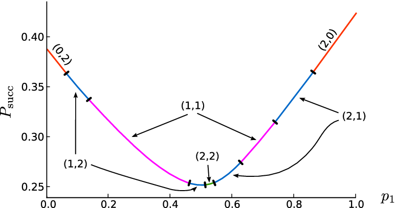
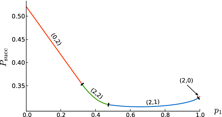
Then, following the discussion in Sec. 3.2, there are six types of optimal USD measurements which differ in the rank of the measurement operators $E_{1}$ and $E_{2}$ . We list these possible types in Table 1.

Table 1: Possible ranks of the measurement operators of the optimal USD measurement in four dimensions (cf. also Sec. 3.2).

$\rank E_{1}$	$\rank E_{2}$	$\rank E_{?}$	$\dim\ker({1\!\!1}-E_{?})$	class	cf. Sec.
0	2	2	2	$[0,2]$	5.1
1	2	2	1	$[1,2]$	6.1
2	2	2	0	$[2,2]$	5.2
1	1	2	2	$[1,1]$	6.2
2	1	2	1	$[1,2]$	6.1
2	0	2	2	$[0,2]$	5.1

The measurements of the class $[0,2]$ and the class $[2,2]$ where already extensively discussed in Sec. 5.1 and Sec. 5.2, respectively. For the class $[1,2]$ , the kernel of $({1\!\!1}-E_{?})$ is one-dimensional. We will consider this class in Sec. 6.1. In the remaining case, where $\rank E_{1}=1=\rank E_{2}$ , the measurement is a von-Neumann measurement (cf. Sec. 3.2). An example of this kind of measurement was first found in Ref. [16]. Sec. 6.2 is devoted for a general treatment of this class.

6.1 The measurement class $[1,2]$

In this class the dimension of $\ker({1\!\!1}-E_{?})$ is $1$ . According to Eq. (12), this kernel is either contained in $\supp\gamma_{1}$ or in $\supp\gamma_{2}$ . Here we focus on $\ker({1\!\!1}-E_{?})\subset\supp\gamma_{1}$ , i.e., to the measurement type $(1,2)$ ; the case of $\ker({1\!\!1}-E_{?})\subset\supp\gamma_{2}$ follows along same lines. Thus there exists an orthonormal basis $({\lvert{\phi}\rangle},{\lvert{\phi^{\perp}}\rangle})$ of $\supp\gamma_{1}$ , such that

E_{?}=\nu{{\lvert{n}\rangle}\!{\langle{n}\rvert}}+{{\lvert{\phi}\rangle}\!{\langle{\phi}\rvert}},

(42)

with ${\lvert{n}\rangle}$ some normalized vector, orthogonal to ${\lvert{\phi}\rangle}$ and $0<\nu<1$ .

6.1.1 The necessary and sufficient conditions

Due to Proposition 3, the operator in Eq. (42) is a valid USD measurement, if and only if $\gamma_{1}({1\!\!1}-E_{?})\gamma_{2}=0$ , i.e.,

\gamma_{1}{{\lvert{\phi^{\perp}}\rangle}\!{\langle{\phi^{\perp}}\rvert}}\gamma_{2}=\nu\gamma_{1}{{\lvert{n}\rangle}\!{\langle{n}\rvert}}\gamma_{2}

(43)

holds. This is equivalent to

\gamma_{1}{\lvert{n}\rangle}=a\gamma_{1}{\lvert{\phi^{\perp}}\rangle}\quad\text{and}\quad\gamma_{2}{\lvert{n}\rangle}=b\gamma_{2}{\lvert{\phi^{\perp}}\rangle}.

(44)

where $a={\langle{\phi^{\perp}}|{n}\rangle}$ and $b=(\nu{\langle{n}|{\phi^{\perp}}\rangle})^{-1}$ . Remember, that due to Theorem 4 we have ${\lvert{n}\rangle}\notin\ker\gamma_{1}$ , i.e., ${\langle{n}|{\phi^{\perp}}\rangle}\neq 0$ . On the other hand, from $\nu<1$ it follows $ab^{*}>1$ and thus ${\lvert{n}\rangle}\notin\vspan\{{\lvert{\phi^{\perp}}\rangle}\}$ , i.e., ${\lvert{n}\rangle}\notin\supp\gamma_{1}$ . Given ${\lvert{\phi^{\perp}}\rangle}$ , we choose the phase of ${\lvert{n}\rangle}$ such that ${\langle{n}|{\phi^{\perp}}\rangle}>0$ .

The conditions in Corollary 9 can now be reduced to simple relations. By multiplying Eq. (25b) from the left with ${{\lvert{\phi^{\perp}}\rangle}\!{\langle{\phi^{\perp}}\rvert}}(\Lambda_{1}-\Lambda_{2})^{-1}$ , this first leads to

{\langle{n}\rvert}\gamma_{2}-\gamma_{1}{\lvert{n}\rangle}=0.

(45)

Now it is straightforward to see that the conditions in Eq. (25) are equivalent to

	$\displaystyle E_{?}(\gamma_{2}-\gamma_{1}){\lvert{n}\rangle}$	$\displaystyle=0,\quad\text{and}$		(46)
	$\displaystyle{\langle{\phi}\rvert}\gamma_{2}-\gamma_{1}{\lvert{\phi}\rangle}$	$\displaystyle\geq 0.$		(47)

By virtue of Eq. (44), we can re-express Eq. (46) in terms of ${\lvert{\phi}\rangle}$ and ${\lvert{\phi^{\perp}}\rangle}$ , yielding

	$\displaystyle\sqrt{{\langle{\phi^{\perp}}\rvert}\gamma_{1}{\lvert{\phi^{\perp}}\rangle}}{\langle{\phi^{\perp}}\rvert}\gamma_{2}{\lvert{\phi}\rangle}$	$\displaystyle=\sqrt{{\langle{\phi^{\perp}}\rvert}\gamma_{2}{\lvert{\phi^{\perp}}\rangle}}{\langle{\phi^{\perp}}\rvert}\gamma_{1}{\lvert{\phi}\rangle},\quad\text{and}$		(48)
	$\displaystyle\frac{a}{b}$	$\displaystyle=\sqrt{\frac{{\langle{\phi^{\perp}}\rvert}\gamma_{2}{\lvert{\phi^{\perp}}\rangle}}{{\langle{\phi^{\perp}}\rvert}\gamma_{1}{\lvert{\phi^{\perp}}\rangle}}}.$		(49)

The last equation enables us to construct $\nu{{\lvert{n}\rangle}\!{\langle{n}\rvert}}$ from

\begin{split}\sqrt{\nu}{\lvert{n}\rangle}&=\sqrt{\nu}(\gamma_{1}+\gamma_{2})^{-1}(\gamma_{1}+\gamma_{2}){\lvert{n}\rangle}\\ &=\sqrt{\nu}(\gamma_{1}+\gamma_{2})^{-1}(a\,\gamma_{1}+b\,\gamma_{2}){\lvert{\phi^{\perp}}\rangle}\\ &=K{\lvert{\phi^{\perp}}\rangle},\end{split}

(50)

where in the last step we used $\sqrt{ab\nu}=1$ and we abbreviated

K=(\gamma_{1}+\gamma_{2})^{-1}\left(\sqrt{a/b}\,\gamma_{1}+\sqrt{b/a}\,\gamma_{2}\right).

(51)

But due to Eq. (49), $\sqrt{a/b}$ is given in terms of ${\lvert{\phi}\rangle}$ and ${\lvert{\phi^{\perp}}\rangle}$ . Note, that $K$ has full rank and hence ensures $\nu\equiv{\langle{\phi^{\perp}}\rvert}K^{\dagger}K{\lvert{\phi^{\perp}}\rangle}>0$ .

We summarize: The optimal USD measurement is of type $(1,2)$ if and only if there exists an orthonormal basis $({\lvert{\phi}\rangle},{\lvert{\phi^{\perp}}\rangle})$ of $\supp\gamma_{1}$ , such that the conditions in Eq. (47), in Eq. (48), and ${\langle{\phi^{\perp}}\rvert}K^{\dagger}K{\lvert{\phi^{\perp}}\rangle}<1$ are satisfied.

6.1.2 Construction of a finite number of candidates for $E_{?}$

In the following we will show, that already Eq. (48) reduces the possible candidates of $\vspan\{{\lvert{\phi}\rangle}\}$ to a finite number and hence the remaining positivity conditions can be easily checked. Eq. (48) is a complex equation. Thus the absolute value and the phase of the left hand side and the right hand side have to be identical. This leads to

	$\displaystyle{\langle{\phi}\rvert}\gamma_{2}{\lvert{\phi^{\perp}}\rangle}{\langle{\phi^{\perp}}\rvert}\gamma_{2}{\lvert{\phi}\rangle}{\langle{\phi^{\perp}}\rvert}\gamma_{1}{\lvert{\phi^{\perp}}\rangle}={\langle{\phi}\rvert}\gamma_{1}{\lvert{\phi^{\perp}}\rangle}{\langle{\phi^{\perp}}\rvert}\gamma_{1}{\lvert{\phi}\rangle}{\langle{\phi^{\perp}}\rvert}\gamma_{2}{\lvert{\phi^{\perp}}\rangle},$		(52)
	$\displaystyle{\langle{\phi^{\perp}}\rvert}\gamma_{2}{\lvert{\phi}\rangle}{\langle{\phi}\rvert}\gamma_{1}{\lvert{\phi^{\perp}}\rangle}\geq 0.$		(53)

Let $({\lvert{s_{1}}\rangle},{\lvert{s_{2}}\rangle})$ be an orthonormal basis of $\supp\gamma_{1}$ , such that $\gamma_{1}{\lvert{s_{i}}\rangle}=g_{1i}{\lvert{s_{i}}\rangle}$ with $g_{11}\geq g_{12}>0$ . We abbreviate $g_{2i}={\langle{s_{i}}\rvert}\gamma_{2}{\lvert{s_{i}}\rangle}>0$ , $g_{\mu}=g_{\mu 1}-g_{\mu 2}$ , and $g_{23}={\langle{s_{1}}\rvert}\gamma_{2}{\lvert{s_{2}}\rangle}.$ We ensure $g_{23}\geq 0$ by choosing a proper global phase of ${\lvert{s_{2}}\rangle}$ . In the case $g_{1}=0$ we use a basis where $g_{23}=0$ .

First we consider, whether ${\lvert{s_{1}}\rangle}$ or ${\lvert{s_{2}}\rangle}$ is a candidate for ${\lvert{\phi}\rangle}$ . In either case, Eq. (48) can only be satisfied, if $g_{23}=0$ . From Eq. (47) we find that ${\lvert{s_{1}}\rangle}$ is a candidate only if $g_{21}\geq g_{11}$ and analogously, ${\lvert{s_{2}}\rangle}$ only if $g_{22}\geq g_{12}$ .

We now assume that neither of the above two cases is optimal. Then any of the remaining bases (apart from global phases) are parametrized by


$\displaystyle{\lvert{\phi}\rangle}$	$\displaystyle=(1+x^{2})^{-\frac{1}{2}}({\lvert{s_{1}}\rangle}+x\mathrm{e}^{i\vartheta}{\lvert{s_{2}}\rangle}),$	(54a)
$\displaystyle{\lvert{\phi^{\perp}}\rangle}$	$\displaystyle=(1+x^{2})^{-\frac{1}{2}}(x\mathrm{e}^{-i\vartheta}{\lvert{s_{1}}\rangle}-{\lvert{s_{2}}\rangle}),$	(54b)

where $x\neq 0$ is real and $-\frac{\pi}{2}\leq\vartheta<\frac{\pi}{2}$ .

Using these definitions, Eq. (53) can be written as

g_{1}g_{23}\sin\vartheta=0\quad\text{and}\quad xg_{1}(xg_{2}+g_{23}(x^{2}-1))\geq 0.

(55)

Let us first discuss the case where $g_{23}\neq 0$ . In this situation we get³³ 3 Remember, that we chose our basis such that $g_{23}\neq 0$ implies $g_{1}\neq 0$ . from Eq. (55) the phase $\vartheta=0$ . The solutions of Eq. (52) are given by the real roots of the polynomial of degree six in $x$ ,

x^{2}g_{1}^{2}(x^{2}g_{21}+g_{22}-2xg_{23})-(xg_{2}+(x^{2}-1)g_{23})^{2}(x^{2}g_{11}+g_{12})=0.

(56)

(Since $g_{23}^{2}g_{12}>0$ , this polynomial cannot be trivial.)

It now remains to consider the special case, where $g_{23}=0$ , but neither ${\lvert{\phi}\rangle}={\lvert{s_{1}}\rangle}$ nor ${\lvert{\phi}\rangle}={\lvert{s_{2}}\rangle}$ is optimal. If $g_{23}=0$ , then Eq. (52) reads

x^{2}(g_{1}^{2}g_{21}-g_{2}^{2}g_{11})=g_{2}^{2}g_{12}-g_{1}^{2}g_{22}.

(57)

Assume that this equation has some solutions where $x$ is real (there might be infinitely many). None of these solutions leads to an optimal measurement, as we exclude by the following argumentation. Neither Eq. (47) nor Eq. (53) depend on $\vartheta$ . From the necessary and sufficient conditions for optimality (cf. end of Sec. 6.1.1), only the condition $\nu\equiv{\langle{\phi^{\perp}}\rvert}K^{\dagger}K{\lvert{\phi^{\perp}}\rangle}<1$ remains to be satisfied. Since Eq. (49) does not depend on $\vartheta$ , also $K$ is independent of $\vartheta$ .

Thus $\nu$ as a function of $\vartheta$ is of the form

\nu(\vartheta)=(1+x^{2})^{-1}\left(x^{2}\kappa_{11}-2\,x\Real(\mathrm{e}^{-i\vartheta}\kappa_{12})+\kappa_{22}\right),

(58)

where we defined $\kappa_{ij}={\langle{s_{i}}\rvert}K^{\dagger}K{\lvert{s_{j}}\rangle}$ . In particular this function is continuous in $\vartheta$ . Assume, for a given $x\neq 0$ (satisfying Eq. (47) and Eq. (48)), there exists some $-\pi/2\leq\vartheta<\pi/2$ , such that $\nu(\vartheta)<1$ . Then there exists an $\epsilon>0$ , such that also $\vartheta+\epsilon<\pi/2$ and $\nu(\vartheta+\epsilon)<1$ . Hence for $\vartheta$ as well as $\vartheta+\epsilon$ all optimality conditions would be satisfied. But for both values, we get a different vector ${\lvert{\phi}\rangle}$ and hence there would be two different operators $E_{?}$ , both being optimal. This is a contradiction to Proposition 11. It follows that for $g_{23}=0$ , only ${\lvert{\phi}\rangle}={\lvert{s_{1}}\rangle}$ and ${\lvert{\phi}\rangle}={\lvert{s_{2}}\rangle}$ can yield an optimal solution.

6.1.3 Summary for measurement type $(1,2)$

Let us briefly summarize the algorithm to obtain the optimal measurement $E_{?}$ for the case where $\rank E_{1}=1$ and $\rank E_{2}=2$ .

We construct some basis $({\lvert{s_{1}}\rangle},{\lvert{s_{2}}\rangle})$ of $\supp\gamma_{1}$ as described in the paragraph below Eq. (53). In a next step, we construct candidates for the basis $({\lvert{\phi}\rangle},{\lvert{\phi^{\perp}}\rangle})$ . There are two cases:

(i)

$g_{23}=0$ . If $g_{21}\geq g_{11}$ , then $({\lvert{\phi}\rangle}={\lvert{s_{1}}\rangle},{\lvert{\phi^{\perp}}\rangle}={\lvert{s_{2}}\rangle})$ is a candidate. If $g_{22}\geq g_{12}$ , then $({\lvert{\phi}\rangle}={\lvert{s_{2}}\rangle},{\lvert{\phi^{\perp}}\rangle}={\lvert{s_{1}}\rangle})$ is a candidate.
(ii)

$g_{23}\neq 0$ . For any real root $x\neq 0$ of the polynomial in Eq. (56), the basis $({\lvert{\phi}\rangle},{\lvert{\phi^{\perp}}\rangle})$ as defined in Eq. (54) is a candidate, where $\vartheta=0$ . A candidate in addition has to satisfy the second part of Eq. (55) and Eq. (47).

For any of the candidate bases (if any), we construct $\sqrt{\nu}{\lvert{n}\rangle}$ using Eq. (50). At most one of the bases will satisfy $\nu\equiv\sqrt{\nu}{\langle{n}|{n}\rangle}\sqrt{\nu}<1$ . If such a basis exists, the optimal measurement is given by Eq. (42).

6.2 The measurement class $[1,1]$

In Sec. 3.2 we have already seen, that if $\rank E_{1}+\rank E_{2}=\rank\gamma_{1}(=\rank\gamma_{2})$ , then both $E_{1}$ and $E_{2}$ are projectors. Hence there are orthonormal bases $({\lvert{\psi_{1}}\rangle},{\lvert{\psi_{1}^{\perp}}\rangle})$ of $\ker\gamma_{2}$ and $({\lvert{\psi_{2}}\rangle},{\lvert{\psi_{2}^{\perp}}\rangle})$ of $\ker\gamma_{1}$ such that

E_{1}={{\lvert{\psi_{1}}\rangle}\!{\langle{\psi_{1}}\rvert}}\quad\text{and}\quad E_{2}={{\lvert{\psi_{2}}\rangle}\!{\langle{\psi_{2}}\rvert}}.

(59)

Since ${1\!\!1}-E_{1}-E_{2}\geq 0$ , necessarily ${\langle{\psi_{1}}|{\psi_{2}}\rangle}=0$ must hold. Using this notation, Eq. (26) is equivalent to


	$\displaystyle{\lvert{{\langle{\psi^{\perp}_{1}}\|{\psi_{2}}\rangle}}\rvert}^{2}{\langle{\psi_{2}}\rvert}\gamma_{2}{\lvert{\psi_{2}}\rangle}\geq{\langle{\psi_{1}^{\perp}}\rvert}\gamma_{1}{\lvert{\psi_{1}^{\perp}}\rangle}$		(60a)
	$\displaystyle{\lvert{{\langle{\psi^{\perp}_{2}}\|{\psi_{1}}\rangle}}\rvert}^{2}{\langle{\psi_{1}}\rvert}\gamma_{1}{\lvert{\psi_{1}}\rangle}\geq{\langle{\psi_{2}^{\perp}}\rvert}\gamma_{2}{\lvert{\psi_{2}^{\perp}}\rangle}$		(60b)
	$\displaystyle{\langle{\psi_{2}^{\perp}}\|{\psi_{1}}\rangle}{\langle{\psi_{1}}\rvert}\gamma_{1}{\lvert{\psi_{1}^{\perp}}\rangle}={\langle{\psi_{2}}\|{\psi_{1}^{\perp}}\rangle}{\langle{\psi_{2}^{\perp}}\rvert}\gamma_{2}{\lvert{\psi_{2}}\rangle},$		(60c)

while Eq. (25b) is satisfied identically. (Note that these equations only follow if all vectors are normalized.)

6.2.1 Construction of a finite number of candidates for $E_{?}$

Let $({\lvert{k_{1i}}\rangle})$ and $({\lvert{k_{2i}}\rangle})$ be Jordan bases (cf. Appendix C) of $\ker\gamma_{1}$ and $\ker\gamma_{2}$ , i.e., $({\lvert{k_{1i}}\rangle})$ and $({\lvert{k_{2i}}\rangle})$ are orthonormal bases of $\ker\gamma_{1}$ and $\ker\gamma_{2}$ , respectively, such that ${\langle{k_{1l}}|{k_{2l}}\rangle}\geq 0$ and for $i\neq j$ one has ${\langle{k_{1i}}|{k_{2j}}\rangle}=0$ . Due to our assumptions in Eq. (41) we have $0<{\langle{k_{1i}}|{k_{2i}}\rangle}<1$ . We choose ${\langle{k_{11}}|{k_{21}}\rangle}\geq{\langle{k_{12}}|{k_{22}}\rangle}$ . In case of degenerate Jordan angles (i.e., ${\langle{k_{11}}|{k_{21}}\rangle}={\langle{k_{12}}|{k_{22}}\rangle}$ ), these bases are not unique and we then choose bases, such that ${\langle{k_{21}}\rvert}\gamma_{1}{\lvert{k_{22}}\rangle}=0$ . We abbreviate

\begin{split}g_{1i}={\langle{k_{2i}}\rvert}\gamma_{1}{\lvert{k_{2i}}\rangle},&\quad g_{2i}={\langle{k_{1i}}\rvert}\gamma_{2}{\lvert{k_{1i}}\rangle},\\ g_{13}={\lvert{{\langle{k_{21}}\rvert}\gamma_{1}{\lvert{k_{22}}\rangle}}\rvert},&\quad g_{23}={\lvert{{\langle{k_{11}}\rvert}\gamma_{2}{\lvert{k_{12}}\rangle}}\rvert},\\ g_{\mu}&=g_{\mu 1}-g_{\mu 2},\end{split}

(61)

and choose the global phases of the vectors ${\lvert{k_{12}}\rangle}$ and ${\lvert{k_{22}}\rangle}$ in such a way that still ${\langle{k_{12}}|{k_{22}}\rangle}>0$ but also $g_{13}\mathrm{e}^{i\varphi}={\langle{k_{21}}\rvert}\gamma_{1}{\lvert{k_{22}}\rangle}$ and $g_{23}\mathrm{e}^{-i\varphi}={\langle{k_{11}}\rvert}\gamma_{2}{\lvert{k_{12}}\rangle}$ , with $0\leq\varphi<\pi$ . We let $\varphi=0$ if $g_{13}=0$ or $g_{23}=0$ . Finally we define $c={\langle{k_{12}}|{k_{22}}\rangle}/{\langle{k_{11}}|{k_{21}}\rangle}$ .

After choosing the Jordan bases, let us first consider the case where ${\lvert{\psi_{1}}\rangle}={\lvert{k_{21}}\rangle}$ . Then one has (fixing the phases) ${\lvert{\psi_{2}}\rangle}={\lvert{k_{12}}\rangle}$ , ${\lvert{\psi_{1}^{\perp}}\rangle}={\lvert{k_{22}}\rangle}$ , and ${\lvert{\psi_{2}^{\perp}}\rangle}={\lvert{k_{11}}\rangle}$ . Eq. (60c) reduces to $cg_{23}=g_{13}$ and $\sin\varphi=0$ . Analogously, in the case ${\lvert{\psi_{1}}\rangle}={\lvert{k_{22}}\rangle}$ , we obtain $cg_{13}=g_{23}$ and $\sin\varphi=0$ .

We now consider the case, where ${\lvert{\psi_{1}}\rangle}$ is not one of the basis vectors ${\lvert{k_{2i}}\rangle}$ . We fix the global phases of ${\lvert{\psi_{\mu}}\rangle}$ and ${\lvert{\psi_{\mu}^{\perp}}\rangle}$ and choose the parametrization

\begin{split}{\lvert{\psi_{1}}\rangle}&=(1+x^{2})^{-\frac{1}{2}}({\lvert{k_{21}}\rangle}+x\mathrm{e}^{i\vartheta}{\lvert{k_{22}}\rangle}),\\ {\lvert{\psi_{1}^{\perp}}\rangle}&=(1+x^{2})^{-\frac{1}{2}}(x\mathrm{e}^{-i\vartheta}{\lvert{k_{21}}\rangle}-{\lvert{k_{22}}\rangle}),\\ {\lvert{\psi_{2}}\rangle}&=(1+c^{2}x^{2})^{-\frac{1}{2}}(-x\mathrm{e}^{-i\vartheta}c{\lvert{k_{11}}\rangle}+{\lvert{k_{12}}\rangle}),\\ {\lvert{\psi_{2}^{\perp}}\rangle}&=(1+c^{2}x^{2})^{-\frac{1}{2}}(-{\lvert{k_{11}}\rangle}-x\mathrm{e}^{i\vartheta}c{\lvert{k_{12}}\rangle}),\end{split}

(62)

with the real parameters $x\neq 0$ and $-\pi/2\leq\vartheta<\pi/2$ .

Using these definitions, Eq. (60c) reads

(x^{2}c^{2}+1)^{2}\left(xg_{1}-\mathrm{e}^{i(\vartheta+\varphi)}g_{13}+x^{2}\mathrm{e}^{-i(\vartheta+\varphi)}g_{13}\right)=\\ c(x^{2}+1)^{2}\left(xcg_{2}-\mathrm{e}^{i(\vartheta-\varphi)}g_{23}+x^{2}c^{2}\mathrm{e}^{-i(\vartheta-\varphi)}g_{23}\right)

(63)

The imaginary part of this equation gives

(x^{2}c^{2}+1)(1+x^{2})\\ \cdot\left[(x^{2}c^{2}+1)\sin(\vartheta+\varphi)g_{13}-(1+x^{2})\sin(\vartheta-\varphi)cg_{23}\right]=0,

(64)

which can only hold if already the term in square brackets is zero. This is the case if and only if

A_{1}\sin\vartheta=A_{2}\cos\vartheta,

(65)

where


$\displaystyle A_{1}$	$\displaystyle=(c(x^{2}+1)g_{23}-(x^{2}c^{2}+1)g_{13})\cos\varphi,$	(66a)
$\displaystyle A_{2}$	$\displaystyle=(c(x^{2}+1)g_{23}+(x^{2}c^{2}+1)g_{13})\sin\varphi.$	(66b)

In order to get the solutions of Eq. (63), we consider now its real part,

(x^{2}c^{2}+1)^{2}(xg_{1}+\cos(\vartheta+\varphi)g_{13}(x^{2}-1))=\\ c(x^{2}+1)^{2}(xcg_{2}+\cos(\vartheta-\varphi)g_{23}(x^{2}c^{2}-1)).

(67)

Using the abbreviations

\begin{split}B_{1}&=(x^{2}c^{2}+1)^{2}xg_{1}-c(x^{2}+1)^{2}xcg_{2},\\ B_{2}&=\left[(x^{2}c^{2}+1)^{2}g_{13}(x^{2}-1)-c(x^{2}+1)^{2}g_{23}(x^{2}c^{2}-1)\right]\cos\varphi,\\ B_{3}&=\left[(x^{2}c^{2}+1)^{2}g_{13}(x^{2}-1)+c(x^{2}+1)^{2}g_{23}(x^{2}c^{2}-1)\right]\sin\varphi,\end{split}

(68)

we get the equivalent expression

B_{1}=B_{3}\sin\vartheta-B_{2}\cos\vartheta.

(69)

Taking the square of this equation, multiplied by $(A_{1}^{2}+A_{2}^{2})$ , we obtain due to Eq. (65) the polynomial (with a degree of at most $8$ in $x^{2}$ )

B_{1}^{2}(A_{1}^{2}+A_{2}^{2})-(A_{1}B_{2}-A_{2}B_{3})^{2}=0.

(70)

This polynomial is trivial if and only if $g_{13}=g_{23}=0$ . (In order to see this, we consider the highest and lowest order term, which only can vanish, if $-(cg_{13}-g_{23})^{2}\cos^{2}\varphi=(cg_{13}+g_{23})^{2}\sin^{2}\varphi$ and if $-(cg_{23}-g_{13})^{2}\cos^{2}\varphi=(cg_{23}+g_{13})^{2}\sin^{2}\varphi$ , respectively. But due to our particular choice of the bases, this can only hold if already $g_{13}=g_{23}=0$ .) It is straightforward to see, that in this case none of the conditions in Eq. (60) depend on $\vartheta$ . Now suppose there is a solution of these conditions with $x\neq 0$ . Then any possible value of $\vartheta$ leads to a different, but optimal measurement, in contradiction to Proposition 11.

In any other situation we get from Eq. (70) a finite number of real solutions $x\neq 0$ . The corresponding value for $\vartheta$ can be obtained as follows. If $A_{1}\neq 0$ , then from Eq. (65) we have $\vartheta=\arctan(A_{2}/A_{1})$ , while if $A_{1}=0$ and $A_{2}\neq 0$ , then $\vartheta=-\pi/2$ . If $A_{1}=A_{2}=0$ , then $\sin\varphi=0$ and

x^{2}=\frac{1}{c}\frac{cg_{23}-g_{13}}{cg_{13}-g_{23}},

(71)

where from $x^{2}>0$ it follows that $(cg_{23}-g_{13})(cg_{13}-g_{23})>0$ . From Eq. (69) we have

2\cos\vartheta\,g_{13}g_{23}(cg_{23}-g_{13})=xc(g_{23}^{2}g_{1}-g_{13}^{2}g_{2}),

(72)

which can be used in order to obtain $\vartheta$ .

6.2.2 Summary for measurement class $[1,1]$

In a first step we construct Jordan bases as described in the first paragraph of Sec. 6.2.1. Then we collect candidates for the bases $({\lvert{\psi_{i}}\rangle},{\lvert{\psi_{i}^{\perp}}\rangle})$ :

(i)

If $\sin\varphi=0$ and $cg_{23}=g_{13}$ , then $({\lvert{\psi_{1}}\rangle}={\lvert{k_{21}}\rangle},{\lvert{\psi_{1}^{\perp}}\rangle}={\lvert{k_{22}}\rangle})$ and $({\lvert{\psi_{2}}\rangle}={\lvert{k_{12}}\rangle},{\lvert{\psi_{2}^{\perp}}\rangle}={\lvert{k_{11}}\rangle})$ is a candidate.
(ii)

If $\sin\varphi=0$ and $cg_{13}=g_{23}$ , then $({\lvert{\psi_{1}}\rangle}={\lvert{k_{22}}\rangle},{\lvert{\psi_{1}^{\perp}}\rangle}={\lvert{k_{21}}\rangle})$ and $({\lvert{\psi_{2}}\rangle}={\lvert{k_{11}}\rangle},{\lvert{\psi_{2}^{\perp}}\rangle}={\lvert{k_{12}}\rangle})$ is a candidate.
(iii)

For any real root $x\neq 0$ of Eq. (70), we get a unique value for $\vartheta$ from Eq. (65) (if $A_{1}\neq 0$ or $A_{2}\neq 0$ ) or from Eq. (72) (if $A_{1}=0$ and $A_{2}=0$ ). If $A_{1}\neq 0$ or $A_{2}\neq 0$ , then in addition Eq. (69) has to hold. For each $(x,\vartheta)$ , we obtain the candidates from Eq. (62).

At most one of the candidates will satisfy Eq. (60a) and Eq. (60b). If such a candidate exists, the optimal measurement is provided by Eq. (59).

6.3 Examples

We want to discuss a few examples of USD in four dimensions, which demonstrate the structure of the previous results. We consider three examples which belong to case [vii] in the flowchart in Fig. 3. Thus these pairs of states in particular are strictly skew and do not posses a common block diagonal structure. In Fig. 1

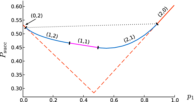
Refer to caption — Figure 1: Optimal success probability of the states given in Eq. (73), depending on the relative probability $p_{1}$ of the occurrence of $\rho_{1}$ (solid line). The dashed lines denote the success probability of single state detection (lower bound) and the dotted line corresponds to a simple upper bound. In brackets we denote the measurement types as defined in Sec. 3.2.

the optimal success probability of the two states

\rho_{1}=\frac{1}{3}\begin{pmatrix}1&0&0&0\\ 0&2&0&0\\ 0&0&0&0\\ 0&0&0&0\end{pmatrix}\quad\text{and}\quad\rho_{2}=\frac{1}{45}\begin{pmatrix}11&10&12&10\\ 10&10&10&10\\ 12&10&14&10\\ 10&10&10&10\end{pmatrix},

(73)

is given in dependence of the a priori probability of $p_{1}$ of $\rho_{1}$ (solid line). Following the results of Sec. 5.1 and Sec. 5.2 we can directly calculate the probability range where single state detection (class $[0,2]$ ) and the fidelity form measurement are optimal (roughly class $[2,2]$ ). The remaining optimal measurements belong to the classes $[1,2]$ or $[1,1]$ which are obtained by following Sec. 6.1 or Sec. 6.2, respectively. We also plotted the “bound triangle” which can be easily calculated for any pair of density operators. The lower bounds correspond to single state detection (dashed lines) and the upper bound connects the points where single state detection stops being optimal (dotted line). The latter one is an upper bound due to the convexity of the success probability function $P_{\mathrm{succ}}(p_{1})$ .

The next example (Fig. 2 (A)) was found by generating “randomly” pairs of density operators. The data of the states is available as supplemental material. This example shows that the measurement types $(1,1)$ , $(1,2)$ , and $(2,1)$ can appear in more than one probability range. This is not possible for the other measurement types. It is also an example for a pair of states, where all possible measurement types can be optimal in some probability range.

The last example (Fig. 2 (B)), given by

\begin{split}\rho_{1}^{\prime}&=\left(\frac{1}{2}+\sqrt{\frac{5}{22}}\right){{\lvert{0}\rangle}\!{\langle{0}\rvert}}+\left(\frac{1}{2}-\sqrt{\frac{5}{22}}\right){{\lvert{1}\rangle}\!{\langle{1}\rvert}},\\ \rho_{2}^{\prime}&=\frac{5}{46}{{\lvert{v}\rangle}\!{\langle{v}\rvert}}+\frac{41}{46}{{\lvert{w}\rangle}\!{\langle{w}\rvert}},\quad\text{with}\\ {\lvert{w}\rangle}&=\frac{1}{2\sqrt{41}}\left((-1)^{1/7}\left((\sqrt{22}+2\sqrt{5}){\lvert{0}\rangle}+(\sqrt{22}-2\sqrt{5}){\lvert{1}\rangle}\right)+2\sqrt{10}\left({\lvert{2}\rangle}+{\lvert{3}\rangle}\right)\right),\\ {\lvert{v}\rangle}&=\frac{1}{\sqrt{10}}\left(((-1)^{4/21})^{*}{\lvert{0}\rangle}+(-1)^{17/21}{\lvert{1}\rangle}+2\sqrt{2}(-1)^{1/5}{\lvert{2}\rangle}\right),\end{split}

(74)

is devoted to show that there is no deeper general structure which optimal measurement classes can be connected with each other. Here, the fidelity form measurement directly follows the single state detection measurement. This example also shows a high asymmetry in the success probability function $P_{\mathrm{succ}}(p_{1})$ .

7 General strategy

In this section we want to summarize the known results for the unambiguous discrimination of two mixed states by suggesting a strategy in order to find the optimal success probability, cf. Fig. 3.

In step [i] we check whether the pair of weighted density operators $\mathcal{S}=(\gamma_{1},\gamma_{2})$ is strictly skew. A pair $\mathcal{S}$ is called strictly skew, if $\supp\gamma_{1}\cap\supp\gamma_{2}=\{0\}$ , $\supp\gamma_{1}\cap\ker\gamma_{2}=\{0\}$ , and $\ker\gamma_{1}\cap\supp\gamma_{2}=\{0\}$ . If the pair fails to be strictly skew, one can use the reduction method described in the discussion of Lemma 7 (Fig. 3 [ii]). After this reduction, it suffices to find the optimal measurement $\mathcal{E}^{\prime}$ of the strictly skew pair $\mathcal{S}^{\prime}$ .

From now on we assume that the states are strictly skew. In the next step (Fig. 3 [iii]) we check with the commutator criteria shown in Ref. [19] whether the two states have an at most two-dimensional common block diagonal structure. If this is the case in Ref. [19] it was shown how to construct diagonalizing Jordan bases, which then can be used to compose the optimal measurement from the pure state case (Fig. 3 [iv]), as shown in Ref. [18, 19].

For states without an at most two-dimensional common block diagonal structure, optimality of one of the two generally solved measurement classes, i.e., single state detection (Proposition 12) or the fidelity form measurement (Proposition 14), can be checked (Fig. 3 [v]). Otherwise the optimal measurement can be calculated if the two states effectively act on a four-dimensional Hilbert-space ( $\dim\supp\mathcal{S}=4$ ). Here the optimal measurement of the two remaining measurement classes $[1,2]$ and $[1,1]$ can be calculated and checked according to Sec. 6.1 and Sec. 6.2, respectively (Fig. 3 [vi]). In principle one could also find optimal measurements of states which have a four-dimensional common block diagonal structure, because then blockwise combination of optimal measurements yields the optimal measurement for the complete states. Unfortunately, there is so far no known constructive method to identify such blocks. This question is left for further investigations.

The last possibility is to check optimality of upper and lower bounds on the optimal success probability (Fig. 3 [viii]). Examples of such bounds were presented e.g. in Ref. [9, 13, 14, 27]. For some of these bounds, optimality conditions are known, while in the remaining cases one can use Corollary 9 in order to check for optimality.

If the procedure sketched here fails to deliver the optimal solution then there is up to now no systematic method known to find an analytic expression for the optimal USD measurement.

8 Conclusions

We analyzed the unambiguous discrimination of two mixed states $\rho_{1}$ and $\rho_{2}$ and the properties of an optimal measurement strategy. We first showed (cf. Proposition 3) that any unambiguous state discrimination measurement is completely determined by the measurement operator $E_{?}$ , the operator which corresponds to the inconclusive measurement result. A further analysis for optimal measurements showed (cf. Theorem 4) that the rank of $E_{?}$ is determined by the structure of the input states, $\rank E_{?}=\rank\rho_{1}\rho_{2}$ .

This fact leads to one of our main results, namely, that the optimal measurement for a given pair of mixed states and given a priori probabilities is unique (cf. Proposition 11). This uniqueness might have interesting consequences, e.g. in the analysis of the “complexity” of the optimal measurement. Interesting questions here are whether the optimal measurement is von-Neumann or whether the optimal measurement is non-local, as e.g. discussed in Ref. [28].

Eldar et al. in Ref. [17] provided necessary and sufficient conditions for a measurement to be optimal, but in many situations this result was not operational. We simplified these optimality conditions in Corollary 9, which now can be applied directly to a given measurement.

As an application of this result, we analyzed the single state detection case, where the measurement only detects one of the two states. Although this measurement may seem to be pathological, it turns out to be always optimal for a finite region of the a priori probabilities of the states. We derive an analytical expression for the bounds of this region.

Finally, we constructed the optimal measurement for the unambiguous discrimination of two mixed states having $\rank\rho_{1}=2=\rank\rho_{2}$ (due to a results by Raynal et al. in Ref. [11], this construction can be extended to the case where one of the density operators has rank 2 and the other state has arbitrary rank). The solution splits into 6 different types, each of them requiring a different treatment. This solution is analytical, but in certain cases the roots of a high order (up to degree 8) polynomial are needed. Due to the complicated structure of this solution it may turn out to be quite difficult to analyze the next step, namely the discrimination of two mixed states with $\rank\rho_{1}=3=\rank\rho_{2}$ .

It would be interesting to find strategies in order to detect symmetries and solvable substructures in unambiguous state discrimination, e.g. to find four-dimensional common block diagonal structures, analogously to the result for two-dimensional common block diagonal structures in Ref. [19]. Also, there are only a few results on the optimal unambiguous discrimination on more than two states [29, 30, 31, 32, 17, 33]. We think that several concepts presented in this contribution may also generalize to the discrimination of many states.

Acknowledgments

We would like to thank J. Bergou, T. Meyer, Ph. Raynal, Z. Shadman, and R. Unanyan for valuable discussions. This work was partially supported by the EU Integrated Projects SECOQC, SCALA, OLAQUI, QICS and by the FWF.

Appendix A Appendix: Technical statements

We put the following two Lemmata for completeness, but without a proof.

Lemma 15.

Let $\mathscr{A}$ , $\mathscr{B}$ and $\mathscr{C}$ be subspaces of ${\mathscr{H}}$ with $\mathscr{A}\perp\mathscr{C}$ and $\mathscr{B}\perp\mathscr{C}$ . Then $\mathscr{A}\cap(\mathscr{B}+\mathscr{C})=\mathscr{A}\cap\mathscr{B}$ .

Lemma 16.

Let $A$ and $B$ be operators on ${\mathscr{H}}$ with $B{\mathscr{H}}\cap\ker A=\{0\}$ . Then $\ker AB=\ker B$ .

The useful Eq. (12) is based on the following

Lemma 17.

Let $X$ be an operator and $(\Pi_{k})$ be a family of projectors with $\ker(\sum_{k}\Pi_{k})=\{0\}$ . For $k\neq l$ , assume that $\Pi_{k}X\Pi_{l}=0$ . (Note that $\Pi_{k}\Pi_{l}\neq 0$ is allowed.). Then $\ker X=\sum_{k}(\ker X\cap\Pi_{k}{\mathscr{H}})$ .

Proof.

The “ $\supset$ ” part is obvious. For the contrary let ${\lvert{\Phi}\rangle}\in\ker X$ . Then there exist vectors ${\lvert{\varphi_{k}}\rangle}\in\Pi_{k}{\mathscr{H}}$ such that ${\lvert{\Phi}\rangle}=\sum_{k}{\lvert{\varphi_{k}}\rangle}$ . We have

\sum_{l}\Pi_{l}X{\lvert{\varphi_{k}}\rangle}=\Pi_{k}X{\lvert{\varphi_{k}}\rangle}=\Pi_{k}X{\lvert{\Phi}\rangle}=0.

(75)

Since $\sum_{k}\Pi_{k}$ has a trivial kernel, it follows that $X{\lvert{\varphi_{k}}\rangle}=0$ , i.e., ${\lvert{\varphi_{k}}\rangle}\in\ker X$ . ∎

The following Lemma lists properties of non-orthogonal projectors, i.e., idempotent operators which are not self-adjoint. Such operators where considered e.g. in Ref. [34, 35]. Each of the statements (ii) – (iv) is a valid definition for the oblique projector, where (ii) is the formal definition, (iii) is an explicit construction and (iv) are the central properties for our purposes.

Lemma 18.

Let $\Lambda$ and $\Pi$ be two (self-adjoint) projectors on ${\mathscr{H}}$ with $\Lambda{\mathscr{H}}\cap(\Pi{\mathscr{H}})^{\perp}=\{0\}$ and $(\Lambda{\mathscr{H}})^{\perp}\cap\Pi{\mathscr{H}}=\{0\}$ . For an operator $Q$ the following statements are equivalent:

(i)

$Q$ is the (unique) oblique projector from $\Lambda{\mathscr{H}}$ to $\Pi{\mathscr{H}}$ .
(ii)

$Q^{2}=Q$ , $Q{\mathscr{H}}=\Pi{\mathscr{H}}$ , and $\ker Q=\ker\Lambda$ .
(iii)

$Q$ is the Moore-Penrose inverse of $\Lambda\Pi$ .
(iv)

$Q\Lambda=Q$ , $\Pi Q=Q$ , $\Lambda Q=\Lambda$ and $Q\Pi=\Pi$ .

Proof.

(ii) formally defines (i). In order to show that (iii) follows from (ii), we write $Q$ in its singular value decomposition, $Q=\sum q_{i}{{\lvert{\pi_{i}}\rangle}\!{\langle{\lambda_{i}}\rvert}}$ with $q_{i}>0$ and $({\lvert{\pi_{i}}\rangle})$ and $({\lvert{\lambda_{i}}\rangle})$ an appropriate pair of orthonormal and complete bases of $\Pi{\mathscr{H}}$ and $\Lambda{\mathscr{H}}$ , respectively. Then $Q^{2}=Q$ is equivalent to ${\langle{\lambda_{k}}|{\pi_{k}}\rangle}=q_{k}^{-1}$ and ${\langle{\lambda_{i}}|{\pi_{j}}\rangle}=0$ for $i\neq j$ . Since $\Lambda\Pi=\sum_{i}q_{i}^{-1}{{\lvert{\lambda_{i}}\rangle}\!{\langle{\pi_{i}}\rvert}}$ , it immediately follows that $Q$ is the Moore-Penrose inverse of $\Lambda\Pi$ .

From the explicit form of the Moore-Penrose inverse, $Q=\sum_{i}{\langle{\lambda_{i}}|{\pi_{i}}\rangle}^{-1}{{\lvert{\pi_{i}}\rangle}\!{\langle{\lambda_{i}}\rvert}}$ , one easily verifies the properties in (iv).

We have from (iv) that $Q{\mathscr{H}}=\Pi Q{\mathscr{H}}\subset\Pi{\mathscr{H}}=Q\Pi{\mathscr{H}}\subset Q{\mathscr{H}}$ and hence $Q{\mathscr{H}}=\Pi{\mathscr{H}}$ and analogously $\ker Q=(Q^{\dagger}{\mathscr{H}})^{\perp}=(\Lambda{\mathscr{H}})^{\perp}=\ker\Lambda$ . Finally, $Q^{2}=Q(\Pi Q)=(Q\Pi)Q=\Pi Q=Q$ . ∎

Appendix B Appendix: Proof of Corollary 9

B.1 Necessity

Let us abbreviate $\bar{\mu}=3-\mu$ , $Z_{\mu}=\Lambda_{\mu}Z\Lambda_{\mu}$ and $Y_{\bar{\mu}}=\Lambda_{\mu}Z\Lambda_{\bar{\mu}}$ . From Theorem 8 it follows that for any optimal measurement we have ( $\mu=1,2$ )


	$\displaystyle Z_{\mu}-\Lambda_{\mu}\gamma_{\mu}\Lambda_{\mu}\geq 0,$		(76a)
	$\displaystyle(Z_{\mu}-\Lambda_{\mu}\gamma_{\mu}\Lambda_{\mu})E_{\mu}=0,$		(76b)

and


$\displaystyle Z_{\mu}(\Lambda_{\mu}-E_{\mu})$	$\displaystyle=Y_{\bar{\mu}}E_{\bar{\mu}}\Lambda_{\mu},$	(77a)
$\displaystyle Y_{\bar{\mu}}(\Lambda_{\bar{\mu}}-E_{\bar{\mu}})$	$\displaystyle=Z_{\mu}E_{\mu}\Lambda_{\bar{\mu}},$	(77b)

where the last two equations follow from $\Lambda_{\mu}ZE_{?}\Lambda_{\nu}=0$ with $E_{?}={1\!\!1}-E_{\mu}-E_{\bar{\mu}}$ . From $Z\geq 0$ we have $Z_{\mu}\geq 0$ and $Y_{\bar{\mu}}=Y^{\dagger}_{\mu}$ . We find

$\displaystyle Z_{\mu}-\Lambda_{\mu}\gamma_{\mu}\Lambda_{\mu}$	$\displaystyle=(\Lambda_{\mu}-E_{\mu})(Z_{\mu}-\gamma_{\mu})(\Lambda_{\mu}-E_{\mu})$	(78)
	$\displaystyle=\Lambda_{\mu}E_{\bar{\mu}}Y_{\bar{\mu}}^{\dagger}(\Lambda_{\mu}-E_{\mu})-(\Lambda_{\mu}-E_{\mu})\gamma_{\mu}(\Lambda_{\mu}-E_{\mu})$
	$\displaystyle=\Lambda_{\mu}E_{\bar{\mu}}\gamma_{\bar{\mu}}E_{\bar{\mu}}\Lambda_{\mu}-(\Lambda_{\mu}-E_{\mu})\gamma_{\mu}(\Lambda_{\mu}-E_{\mu})$
	$\displaystyle=\Lambda_{\mu}E_{?}\gamma_{\bar{\mu}}E_{?}\Lambda_{\mu}-\Lambda_{\mu}E_{?}\gamma_{\mu}E_{?}\Lambda_{\mu}.$

Thus Eq. (26a), Eq. (26b) follow from Eq. (76a). From Eq. (76b) we have

\Lambda_{\mu}E_{?}(\gamma_{\bar{\mu}}-\gamma_{\mu})E_{?}E_{\mu}=0.

(79)

Combining Eq. (77a) and Eq. (77b) we obtain

Y_{\bar{\mu}}\Lambda_{\mu}=Z_{\mu}E_{\mu}\Lambda_{\bar{\mu}}\Lambda_{\mu}+Z_{\mu}(\Lambda_{\mu}-E_{\mu})

(80)

and hence from Eq. (77a) and due to Eq. (76b),

$\displaystyle\Lambda_{\bar{\mu}}Z_{\mu}(\Lambda_{\mu}-E_{\mu})$	$\displaystyle=(Y_{\mu}\Lambda_{\bar{\mu}})^{\dagger}E_{\bar{\mu}}\Lambda_{\mu}$	(81)
	$\displaystyle=\Lambda_{\bar{\mu}}\Lambda_{\mu}E_{\bar{\mu}}\gamma_{\bar{\mu}}E_{\bar{\mu}}\Lambda_{\mu}+(\Lambda_{\bar{\mu}}-E_{\bar{\mu}})\gamma_{\bar{\mu}}E_{\bar{\mu}}\Lambda_{\mu}$
	$\displaystyle=\Lambda_{\bar{\mu}}(\Lambda_{\mu}-E_{\mu})Z_{\mu}(\Lambda_{\mu}-E_{\mu})+(\Lambda_{\bar{\mu}}-E_{\bar{\mu}})\gamma_{\bar{\mu}}E_{\bar{\mu}}\Lambda_{\mu},$

where in the last step we used the result from Eq. (78). Thus we have found $\Lambda_{\bar{\mu}}E_{\mu}\gamma_{\mu}(\Lambda_{\mu}-E_{\mu})=(\Lambda_{\bar{\mu}}-E_{\bar{\mu}})\gamma_{\bar{\mu}}E_{\bar{\mu}}\Lambda_{\mu}$ , i.e., Eq. (26c) follows.

This equation together with Eq. (79) for $\mu=1$ and $\mu=2$ , finally yields Eq. (25b).

B.2 Sufficiency

We first get rid of the non-skew parts of $\mathcal{S}$ :

Lemma 19.

With the definitions and preliminaries as in Proposition 6, if $E_{?}$ is a proper USD measurement of $\mathcal{S}$ and satisfies Eq. (25) for $\mathcal{S}$ , then $E_{?}^{\mathrm{skew}}=E_{?}+({1\!\!1}-\Pi_{\mathrm{skew}})$ is a proper USD measurement of $\mathcal{S}^{\mathrm{skew}}$ and satisfies Eq. (25) for $\mathcal{S}^{\mathrm{skew}}$ .

Hence, if we further show, that from the second part of the Lemma, it follows that $E_{?}^{\mathrm{skew}}$ is optimal for $\mathcal{S}^{\mathrm{skew}}$ , then we have due to Proposition 6, that also $E_{?}$ is optimal for $\mathcal{S}$ .

Proof of Lemma 19.

We denote by $\Sigma_{1}$ the projector onto $\supp\gamma_{1}\cap\ker\gamma_{2}$ , by $\Sigma_{2}$ the projector onto $\supp\gamma_{2}\cap\ker\gamma_{1}$ and by $\Pi_{\mu}$ the projector onto $\supp\gamma_{\mu}$ . Then multiplication of Eq. (25a) by $\Sigma_{1}$ yields

\Sigma_{1}E_{?}\gamma_{2}E_{?}\Sigma_{1}-\Sigma_{1}E_{?}\gamma_{1}E_{?}\Sigma_{1}\geq 0.

(82)

Since for a USD measurement $\Pi_{1}E_{?}\gamma_{2}=\Pi_{1}\gamma_{2}$ , we have $\Sigma_{1}\gamma_{2}=0$ and only the second term remains, which henceforth must vanish. This yields $\sqrt{\gamma_{1}}E_{?}\Sigma_{1}=0$ or equivalently $\Pi_{1}E_{?}\Sigma_{1}=0$ . A further multiplication from the left by $\Sigma_{1}$ together with the property $E_{?}\geq 0$ proves that $E_{?}\Sigma_{1}=0$ . An analogous argument can be used in order to show $E_{?}\Sigma_{2}=0$ . Now, following the same lines of argument as in the proof of Proposition 6, it follows that $E_{?}^{\mathrm{skew}}$ is a proper USD measurement for $\mathcal{S}^{\mathrm{skew}}$ .

From $E_{?}\Sigma_{\mu}=0$ it in particular follows that $E_{?}(\gamma_{2}-\gamma_{1})E_{?}=E_{?}^{\mathrm{skew}}\Pi_{\mathrm{skew}}(\gamma_{2}-\gamma_{1})\Pi_{\mathrm{skew}}E_{?}^{\mathrm{skew}}$ . Using

\ker\Pi_{\mathrm{skew}}\gamma_{\mu}\Pi_{\mathrm{skew}}=\ker\gamma_{\mu}({1\!\!1}-\Sigma_{\mu})=\Sigma_{\mu}{\mathscr{H}}\oplus\ker\gamma_{\mu},

(83)

it is now straightforward to show that $E_{?}^{\mathrm{skew}}$ satisfies Eq. (25) for $\mathcal{S}^{\mathrm{skew}}$ . ∎

It remains to consider the case where $\supp\gamma_{1}\cap\ker\gamma_{2}=\{0\}=\supp\gamma_{2}\cap\ker\gamma_{1}$ . We define $R_{\mu}$ to be the oblique projector from $\ker\gamma_{\bar{\mu}}$ to $\ker\gamma_{\mu}$ . Note that $R_{\mu}=R_{\bar{\mu}}^{\dagger}$ . We furthermore denote by $Q_{\mu}$ the oblique projector from $\ker\gamma_{\bar{\mu}}\cap\supp\mathcal{S}$ to $\supp\gamma_{\mu}\cap(\ker\gamma_{1}+\ker\gamma_{2})$ . Then the multiplication of Eq. (25b) by $Q_{\mu}^{\dagger}$ from the left and by $Q_{\mu}$ from the right yields

\Lambda_{\mu}E_{?}(\gamma_{\bar{\mu}}-\gamma_{\mu})E_{?}E_{\mu}=0.

(84)

Let us define

	$\displaystyle V_{\mu}$	$\displaystyle=\Lambda_{\mu}E_{?}(\gamma_{\bar{\mu}}-\gamma_{\mu})E_{?}\Lambda_{\mu}+\Lambda_{\mu}\gamma_{\mu}\Lambda_{\mu},$		(85)
	$\displaystyle W_{\bar{\mu}}$	$\displaystyle=(R_{\bar{\mu}}(\Lambda_{\bar{\mu}}-E_{\bar{\mu}})+\Lambda_{\mu}E_{\bar{\mu}})V_{\bar{\mu}}.$		(86)

Then, using Eq. (26c),(84), we have

$\displaystyle V_{\mu}(\Lambda_{\mu}-E_{\mu})$	$\displaystyle=\Lambda_{\mu}E_{?}(\gamma_{\bar{\mu}}-\gamma_{\mu})E_{?}\Lambda_{\mu}+\Lambda_{\mu}\gamma_{\mu}E_{?}\Lambda_{\mu}$	(87)
	$\displaystyle=\Lambda_{\mu}E_{?}\gamma_{\bar{\mu}}E_{?}\Lambda_{\mu}+E_{\mu}\gamma_{\mu}E_{?}\Lambda_{\mu}$
	$\displaystyle=-\Lambda_{\mu}E_{\bar{\mu}}\gamma_{\bar{\mu}}E_{?}\Lambda_{\mu}-R_{\bar{\mu}}E_{?}\gamma_{\mu}E_{?}\Lambda_{\mu}$
	$\displaystyle=-(\Lambda_{\mu}E_{\bar{\mu}}+R_{\bar{\mu}}E_{?})\gamma_{\bar{\mu}}E_{?}\Lambda_{\mu}$
	$\displaystyle=(\Lambda_{\mu}E_{\bar{\mu}}+R_{\bar{\mu}}(\Lambda_{\bar{\mu}}-E_{\bar{\mu}}))\gamma_{\bar{\mu}}E_{\bar{\mu}}\Lambda_{\mu}$
	$\displaystyle=W_{\bar{\mu}}E_{\bar{\mu}}\Lambda_{\mu}.$

And a similar equation holds for $W_{\bar{\mu}}$ :

$\displaystyle W_{\bar{\mu}}(\Lambda_{\bar{\mu}}-E_{\bar{\mu}})=$	$\displaystyle R_{\bar{\mu}}E_{?}(\gamma_{\mu}-\gamma_{\bar{\mu}})E_{?}\Lambda_{\bar{\mu}}+R_{\bar{\mu}}(\Lambda_{\bar{\mu}}-E_{\bar{\mu}})\gamma_{\bar{\mu}}(\Lambda_{\bar{\mu}}-E_{\bar{\mu}})$	(88)
	$\displaystyle+\Lambda_{\mu}E_{\bar{\mu}}\gamma_{\bar{\mu}}(\Lambda_{\bar{\mu}}-E_{\bar{\mu}})$
$\displaystyle=$	$\displaystyle R_{\bar{\mu}}E_{?}\gamma_{\mu}E_{?}\Lambda_{\bar{\mu}}-\Lambda_{\mu}E_{?}\gamma_{\mu}E_{?}\Lambda_{\bar{\mu}}$
$\displaystyle=$	$\displaystyle-(-E_{\mu}-(\Lambda_{\mu}-E_{\mu}))\gamma_{\mu}E_{\mu}\Lambda_{\bar{\mu}}$
$\displaystyle=$	$\displaystyle V_{\mu}E_{\mu}\Lambda_{\bar{\mu}}.$

We combine these two equations and find $W_{\bar{\mu}}=V_{\mu}(E_{\mu}\Lambda_{\bar{\mu}}+(\Lambda_{\mu}-E_{\mu})R_{\bar{\mu}})$ , i.e., in comparison with the definition in Eq. (86), $W_{\bar{\mu}}=W_{\mu}^{\dagger}$ . Furthermore, we have $W_{1}V_{1}^{-}V_{1}=W_{1}$ and $V_{2}=W_{1}V_{1}^{-}W_{1}^{\dagger}$ , where $V_{1}^{-}$ denotes the inverse of $V_{1}$ on its support. (The second identity follows from $W_{1}V_{1}^{-}W_{1}^{\dagger}=W_{1}(\Lambda_{1}-E_{1})R_{2}+W_{1}E_{1}\Lambda_{2}$ .)

We construct the operator $Z$ as $Z=TV_{1}T^{\dagger}$ with $T=Q_{1}+Q_{2}W_{1}V_{1}^{-}$ . Since $V_{1}\geq 0$ we have $Z\geq 0$ . From our previous considerations, $\Lambda_{\mu}Z\Lambda_{\mu}=V_{\mu}$ and $\Lambda_{\mu}Z\Lambda_{\bar{\mu}}=W_{\bar{\mu}}$ follows. Then using Eq. (26a), Eq. (26b), and Eq. (84) it is now straightforward to verify that $Z$ satisfies the conditions in Eq. (24b) of Theorem 8.

It remains to show that $ZE_{?}=0$ . First, with $\Pi_{\parallel}$ the projector onto $\supp\gamma_{1}\cap\supp\gamma_{2}$ , we have $ZE_{?}\Pi_{\parallel}=Z\Pi_{\parallel}=0$ due to $\Pi_{\parallel}Q_{\mu}=0$ . Analogously with $\Pi_{\perp}$ the projector onto $\ker\mathcal{S}$ , $ZE_{?}\Pi_{\perp}=Z\Pi_{\perp}=0$ . Thus we only need to show that $\Lambda_{\mu}ZE_{?}\Lambda_{\nu}=0$ . But this follows from Eq. (87) and Eq. (88).

Appendix C Appendix: Construction of Jordan bases

In this Appendix an explicit construction of Jordan bases (also sometimes called canonical bases) of two subspaces $\mathscr{A}$ and $\mathscr{B}$ of $\mathbb{C}^{d}$ is given (cf. also Ref. [36, 9, 19, 18]). Jordan bases are orthonormal bases $({\lvert{a_{i}}\rangle})$ of $\mathscr{A}$ and $({\lvert{b_{j}}\rangle})$ of $\mathscr{B}$ , such that ${\langle{a_{i}}|{b_{j}}\rangle}=0$ for all $i\neq j$ and ${\langle{a_{k}}|{b_{k}}\rangle}\geq 0$ for all $k$ . With $S_{\mathscr{A}}$ we denote the $d\times n_{\mathscr{A}}$ dimensional matrix where the columns are given by the $n_{\mathscr{A}}$ basis vectors of some orthonormal basis of $\mathscr{A}$ . Analogously we define $S_{\mathscr{B}}$ and $n_{\mathscr{B}}$ by using $\mathscr{B}$ .

Consider a singular value decomposition of

S_{\mathscr{A}}^{\dagger}S_{\mathscr{B}}=U_{\mathscr{A}}DU_{\mathscr{B}}^{\dagger},\quad\text{i.e.,}\quad\left(S_{\mathscr{A}}U_{\mathscr{A}}\right)^{\dagger}\left(S_{\mathscr{B}}U_{\mathscr{B}}\right)=D,

(89)

where $D$ is a $n_{\mathscr{A}}\times n_{\mathscr{B}}$ dimensional diagonal matrix. $U_{\mathscr{A}}$ and $U_{\mathscr{B}}$ are unitary matrices. Let us denote the $i$ -th column of $S_{\mathscr{A}}U_{\mathscr{A}}$ by ${\lvert{a_{i}}\rangle}$ and the $j$ -th column of $S_{\mathscr{B}}U_{\mathscr{B}}$ by ${\lvert{b_{j}}\rangle}$ . Then $({\lvert{a_{i}}\rangle})$ and $({\lvert{b_{j}}\rangle})$ are Jordan bases of $\mathscr{A}$ and $\mathscr{B}$ .

References

[1] C. W. Helstrøm, Quantum Detection and Estimation Theory, Acad. Press, New York, 1976.
[2] U. Herzog, J. A. Bergou, Distinguishing mixed quantum states: Minimum-error discrimination versus optimum unambiguous discrimination, Phys. Rev. A 70 (2) (2004) 022302.
[3] I. D. Ivanovic, How to differentiate between non-orthogonal states, Phys. Lett. A 123 (6) (1987) 257–259.
[4] D. Dieks, Overlap and distinguishability of quantum states, Phys. Lett. A 126 (5-6) (1988) 303–306.
[5] A. Peres, How to differentiate between non-orthogonal states, Phys. Lett. A 128 (1988) 19.
[6] G. Jaeger, A. Shimony, Optimal distinction between two non-orthogonal quantum states, Phys. Lett. A 197 (2) (1995) 83–87.
[7] C. H. Bennett, T. Mor, J. A. Smolin, Parity bit in quantum cryptography, Phys. Rev. A 54 (4) (1996) 2675–2684.
[8] Y. Sun, J. A. Bergou, M. Hillery, Optimum unambiguous discrimination between subsets of nonorthogonal quantum states, Phys. Rev. A 66 (3) (2002) 032315.
[9] T. Rudolph, R. W. Spekkens, P. S. Turner, Unambiguous discrimination of mixed states, Phys. Rev. A 68 (1) (2003) 010301(R).
[10] J. A. Bergou, U. Herzog, M. Hillery, Quantum filtering and discrimination between sets of boolean functions, Phys. Rev. Lett. 90 (25) (2003) 257901.
[11] P. Raynal, N. Lütkenhaus, S. J. van Enk, Reduction theorems for optimal unambiguous state discrimination of density matrices, Phys. Rev. A 68 (2) (2003) 022308.
[12] J. A. Bergou, U. Herzog, M. Hillery, Optimal unambiguous filtering of a quantum state: An instance in mixed state discrimination, Phys. Rev. A 71 (4) (2005) 042314.
[13] U. Herzog, J. A. Bergou, Optimum unambiguous discrimination of two mixed quantum states, Phys. Rev. A 71 (5) (2005) 050301(R).
[14] P. Raynal, N. Lütkenhaus, Optimal unambiguous state discrimination of two density matrices: Lower bound and class of exact solutions, Phys. Rev. A 72 (2005) 022342, 049909(E).
[15] U. Herzog, Optimum unambiguous discrimination of two mixed states and application to a class of similar states, Phys. Rev. A 75 (5) (2007) 052309.
[16] P. Raynal, N. Lütkenhaus, Optimal unambiguous state discrimination of two density matrices: A second class of exact solutions, Phys. Rev. A 76 (2007) 052322.
[17] Y. C. Eldar, M. Stojnic, B. Hassibi, Optimal quantum detectors for unambiguous detection of mixed states, Phys. Rev. A 69 (6) (2004) 062318.
[18] J. A. Bergou, E. Feldman, M. Hillery, Optimal unambiguous discrimination of two subspaces as a case in mixed-state discrimination, Phys. Rev. A 73 (3) (2006) 032107.
[19] M. Kleinmann, H. Kampermann, P. Raynal, D. Bruß, Commutator relations reveal solvable structures in unambiguous state discrimination, J. Phys. A: Math. Theor. 40 (36) (2007) F871–F878.
[20] L. P. Hughston, R. Jozsa, W. K. Wootters, A complete classification of quantum ensembles having a given density matrix, Phys. Lett. A 183 (1) (1993) 14–18.
[21] A. Bassi, G. Ghirardi, A general scheme for ensemble purification, Phys. Lett. A 309 (1-2) (2003) 24–28.
[22] M. Kleinmann, H. Kampermann, T. Meyer, D. Bruß, Physical purification of quantum states, Phys. Rev. A 73 (6) (2006) 062309.
[23] M. Kleinmann, H. Kampermann, T. Meyer, D. Bruß, Purifying and reversible physical processes, Appl. Phys. B 86 (3) (2007) 371–375.
[24] A. Uhlmann, The ”transition probability” in the state space of a *-algebra, Rep. Math. Phys. 9 (1976) 273–279.
[25] R. Jozsa, Fidelity for mixed quantum states, J. Mod. Opt. 41 (12) (1994) 2315–2323.
[26] D. Bures, An extension of kakutani’s theorem on infinite product measures to the tensor product of semifinite w*-algebras, Transactions of the American Mathematical Society 135 (1969) 199–212.
[27] X.-F. Zhou, Y.-S. Zhang, G.-C. Guo, Unambiguous discrimination of mixed states: A description based on system-ancilla coupling, Phys. Rev. A 75 (5) (2007) 052314.
[28] M. Kleinmann, H. Kampermann, D. Bruß, Generalization of quantum-state comparison, Phys. Rev. A 72 (3) (2005) 032308.
[29] A. Chefles, Unambiguous discrimination between linearly independent quantum states, Phys. Lett. A 239 (6) (1998) 339–347.
[30] A. Chefles, S. M. Barnett, Optimum unambiguous discrimination between linearly independent symmetric states, Phys. Lett. A 250 (4-6) (1998) 223–229.
[31] A. Peres, D. R. Terno, Optimal distinction between non-orthogonal quantum states, J. Phys. A: Math. Gen. 31 (1998) 7105–7111.
[32] C. Zhang, Y. Feng, M. Ying, Unambiguous discrimination of mixed quantum states, Phys. Lett. A 353 (2006) 300–306.
[33] B. F. Samsonov, Optimal positive-operator-valued measures for unambiguous state discrimination, arXiv:0806.2699 (2009).
[34] S. N. Afriat, Orthogonal and oblique projectors and the characteristics of pairs of vectors spaces, Proc. Camb. Philos. Soc. 53 (1957) 800–816.
[35] T. N. E. Greville, Solutions of the matrix equation $XAX=X$ , and relations between oblique and orthogonal projectors, SIAM J. Appl. Math. 26 (4) (1974) 828–832.
[36] G. W. Stewart, J.-G. Sun, Matrix Pertubation Theory, Acad. Press, San Diego, 1990.

Structural approach to unambiguous discrimination of two mixed quantum states

Abstract

1 Introduction

2 Defining properties of USD

2.1 Main definitions

Definition 1.

2.2 Trivial subspaces

Proposition 2 (cf. Theorem 1 in Ref. [11]).

Proof.

2.3 The role of E?E_{?}

Proposition 3.

Proof.

3 Simple properties of optimal measurements

Theorem 4.

Proof.

3.1 Orthogonal subspaces

Lemma 5.

Proof.

Proposition 6 (cf. Theorem 2 in Ref. [11]).

Proof.

Lemma 7.

Proof.

3.2 Classification of USD measurements

4 The optimality conditions by Eldar, Stojnic & Hassibi

Theorem 8 (Eldar, Stojnic & Hassibi [17]).

Corollary 9.

Lemma 10.

Proof.

Proposition 11.

5 Two special classes of optimal measurements

5.1 Single state detection

Proposition 12.

Proof.

5.2 Fidelity form measurement

Lemma 13.

Proof.

Proposition 14 (cf. Theorem 4 in Ref. [14]).

Proof.

6 Solution in four dimensions

6.1 The measurement class [1,2][1,2]

6.1.1 The necessary and sufficient conditions

6.1.2 Construction of a finite number of candidates for E?E_{?}

6.1.3 Summary for measurement type (1,2)(1,2)

6.2 The measurement class [1,1][1,1]

6.2.1 Construction of a finite number of candidates for E?E_{?}

6.2.2 Summary for measurement class [1,1][1,1]

6.3 Examples

7 General strategy

8 Conclusions

Acknowledgments

Appendix A Appendix: Technical statements

Lemma 15.

Lemma 16.

Lemma 17.

Proof.

Lemma 18.

Proof.

Appendix B Appendix: Proof of Corollary 9

B.1 Necessity

B.2 Sufficiency

Lemma 19.

Proof of Lemma 19.

Appendix C Appendix: Construction of Jordan bases

References

2.3 The role of $E_{?}$

6.1 The measurement class $[1,2]$

6.1.2 Construction of a finite number of candidates for $E_{?}$

6.1.3 Summary for measurement type $(1,2)$

6.2 The measurement class $[1,1]$

6.2.1 Construction of a finite number of candidates for $E_{?}$

6.2.2 Summary for measurement class $[1,1]$