Geometric measure of entanglement and shared quantum states

Levon Tamaryan Affiliation: Physics Department, Yerevan State University, Yerevan, 375025, Armenia DaeKil Park Affiliation: Department of Physics, Kyungnam University, Masan, 631-701, Korea Jin-Woo Son Affiliation: Department of Mathematics, Kyungnam University, Masan, 631-701, Korea Sayatnova Tamaryan Affiliation: Theory Department, Yerevan Physics Institute, Yerevan, 375036, Armenia

Abstract

We give an explicit expression for the geometric measure of entanglement for three qubit states that are linear combinations of four orthogonal product states. It turns out that the geometric measure for these states has three different expressions depending on the range of definition in parameter space. Each expression of the measure has its own geometrically meaningful interpretation. Such an interpretation allows oneself to take one step toward a complete understanding for the general properties of the entanglement measure. The states that lie on joint surfaces separating different ranges of definition, designated as shared states, seem to have particularly interesting features. The properties of the shared states are fully discussed.

pacs

03.67.Mn, 02.10.Yn, 02.40.Dr

I Introduction

Entanglement is the most intriguing feature of quantum mechanics and a key resource in quantum information science. One of the main goals in these theories is to develop a comprehensive theory of multipartite entanglement. Various entanglement measures have been invented to quantify the multi-particle entanglement [1, 2, 3, 4, 5, 6, 7] but none of them were able to suggest a method for calculating a measure of multipartite systems. This mathematical difficulty is the main obstacle to elaborate a theory of multi-particle entanglement.

In this paper, we present the first calculation of the geometric measure of entanglement [7, 8, 9] for three qubit states which are expressed as linear combinations of four given orthogonal product states. Any pure three qubit state can be written in terms of five preassigned orthogonal product states [10] via Schmidt decomposition. Thus the states discussed here are more general states compared to the well-known GHZ [11] and W [12] states.

The reason for using the geometric measure of entanglement is that it is suitable for any partite system regardless of its dimensions. However, analytical computation for generic states still remains as a great challenge. The measure depends on entanglement eigenvalue $\Lambda_{\max}^{2}$ and can be derived from the formula $E_{g}(\psi)=1-\Lambda_{\max}^{2}$ . For pure states, the entanglement eigenvalue is equal to the maximal overlap of a given state with any complete product state. This measure has the following remarkable properties:

i) it has an operational treatment. The same overlap $\Lambda_{\max}^{2}$ defines Groverian measure of entanglement [13, 14] which has been introduced later in operational terms. In other words, it quantifies how well a given state serves as an input state to Grover’s search algorithm [15]. From this view, Groverian measure can be regarded as an operational treatment of the geometric measure.

ii) it has identified irregularity in channel capacity additivity [16]. Using this measure, one can show that a family of quantities, which were thought to be additive in an earlier papers, actually are not. For example, it is natural to conjecture that preparing two pairs of entangled particles should give us twice the entanglement of one pair and, similarly, using a channel twice doubles its capacity. However, this conjecture claiming additivity has proved to be wrong in some cases.

iii) it has useful connections to other entanglement measures and gives rise to a lower bound on the relative entropy of entanglement [17] and generalized robustness [18]. For certain pure states the first lower bound is saturated and thus their relative entropy of entanglement can be deduced from their geometric measure of entanglement. The second lower bound to generalized robustness can be express in terms of $\Lambda_{\max}^{2}$ directly.

Owing to these features, the geometric measure can play an important role in the investigation of different problems related to entanglement. For example, the entanglement of two distinct multipartite bound entangled states can be determined analytically in terms of a geometric measure of entanglement [19]. Recently, the same measure has been used to understand the physical implication of Zamolodchikov’s c-theorem [20] more deeply. It is an important application regarding the quantum information techniques in the effect of renormalization group in field theories [21]. Thus it is natural that geometric measure of entanglement is an object of intense interest and in some recent works revised [22] and generalized [23] versions of the geometric measure were presented.

The progress made to date allows oneself to calculate the geometric measure of entanglement for pure three qubit systems [24]. The basic idea is to use $(n-1)$ -qubit mixed states to calculate the geometric measure of $n$ -qubit pure states. In the case of three qubits this idea converts the task effectively into the maximization of the two-qubit mixed state over product states and yields linear eigenvalue equations [25]. The solution of these linear eigenvalue equations reduces to the root finding for algebraic equations of degree six. However, three-qubit states containing symmetries allow complete analytical solutions and explicit expressions as the symmetry reduces the equations of degree six to the quadratic equations. Analytic expressions derived in this way are unique and the presented effective method can be applied for extended quantum systems. Our aim is to derive analytic expressions for a wider class of three qubit systems and in this sense this work is the continuation of Ref.[25].

We consider most general W-type three qubit states that allow to derive analytic expressions for entanglement eigenvalue. These states can be expressed as linear combinations of four given orthogonal product states. If any of coefficients in this expansion vanishes, then one obtains the states analyzed in [25]. Notice that arbitrary linear combinations of five product states [10] give a couple of algebraic equations of degree six. Hence Évariste Galois’s theorem does not allow to get analytic expressions for these states except some particular cases.

We derive analytic expressions for an entanglement eigenvalue. Each expression has its own applicable domain depending on state parameters and these applicable domains are split up by separating surfaces. Thus the geometric measure distinguishes different types of states depending on the corresponding applicable domain. States that lie on separating surfaces are shared by two types of states and acquire new features.

In Section II we derive stationarity equations and their solutions. In Section III we specify three qubit states under consideration and find relevant quantities. In Section IV we calculate entanglement eigenvalues and present explicit expressions. In Section V we separate the validity domains of the derived expressions. In Section VI we discuss shared states. In section VII we make concluding remarks.

II Stationarity equations

In this section we briefly review the derivation of the stationarity equations and their general solutions [25]. Denote by $\rho^{ABC}$ the density matrix of the three-qubit pure state and define the entanglement eigenvalue $\Lambda_{\max}^{2}$ [7]

\Lambda_{\max}^{2}=\max_{\varrho^{1}\varrho^{2}\varrho^{3}}\mathrm{tr}\left(\rho^{ABC}\varrho^{1}\otimes\varrho^{2}\otimes\varrho^{3}\right),

(1)

where the maximization runs over all normalized complete product states. Theorem 1 of Ref.[24] states that the maximization of a pure state over a single qubit state can be completely derived by using a particle traced over density matrix. Hence the theorem allows us to re-express the entanglement eigenvalue by reduced density matrix $\rho^{AB}$ of qubits A and B

\Lambda_{\max}^{2}=\max_{\varrho^{1}\varrho^{2}}\mathrm{tr}\left(\rho^{AB}\varrho^{1}\otimes\varrho^{2}\right).

(2)

Now we introduce four Bloch vectors:

1) ${\bm{r}}_{A}$ for the reduced density matrix $\rho^{A}$ of the qubit A,

2) ${\bm{r}}_{B}$ for the reduced density matrix $\rho^{B}$ of the qubit B,

3) ${\bm{u}}$ for the single qubit state $\varrho^{1}$ ,

4) ${\bm{v}}$ for the single qubit state $\varrho^{2}$ .

Then the expression for entanglement eigenvalue (2) takes the form

\Lambda_{\max}^{2}=\frac{1}{4}\max_{u^{2}=v^{2}=1}\left(1+{\bm{u}}\cdot{\bm{r}}_{A}+{\bm{v}}\cdot{\bm{r}}_{B}+g_{ij}\,u_{i}v_{j}\right),

(3)

where(summation on repeated indices $i$ and $j$ is understood)

g_{ij}=\mathrm{tr}(\rho^{AB}\sigma_{i}\otimes\sigma_{j})

(4)

and $\sigma_{i}$ ’s are Pauli matrices. The closest product state satisfies the stationarity conditions

{\bm{r}}_{A}+g{\bm{v}}=\lambda_{1}{\bm{u}},\quad{\bm{r}}_{B}+g^{T}{\bm{u}}=\lambda_{2}{\bm{v}},

(5)

where Lagrange multipliers $\lambda_{1}$ and $\lambda_{2}$ enforce the unit Bloch vectors ${\bm{u}}$ and ${\bm{v}}$ . The solutions of Eq.(5) are

{\bm{u}}=\left(\lambda_{1}\lambda_{2}\openone-g\,g^{T}\right)^{-1}\left(\lambda_{2}{\bm{r}}_{A}+g\,{\bm{r}}_{B}\right),\quad{\bm{v}}=\left(\lambda_{1}\lambda_{2}\openone-g^{T}g\right)^{-1}\left(\lambda_{1}{\bm{r}}_{B}+g^{T}{\bm{r}}_{A}\right).

(6)

Unknown Lagrange multipliers are defined by equations

u^{2}=1,\quad v^{2}=1.

(7)

In general, Eq.(7) gives algebraic equations of degree six. The reason for this is that stationarity equations define all extremes of the reduced density matrix $\rho^{AB}$ over product states, regardless of them being global or local. And the degree of the algebraic equations is the number of possible extremes.

Eq.(6) contains valuable information. It provides solid bases for a new numerical approach. This can be compared with the numerical calculations based on other technique [26].

III Three Qubit State

We consider W-type state

|\psi\rangle=a|100\rangle+b|010\rangle+c|001\rangle+d|111\rangle,

(8)

where free parameters $a,b,c,d$ satisfy the normalization condition $a^{2}+b^{2}+c^{2}+d^{2}=1$ . Without loss of generality we consider only the case of positive parameters $a,b,c,d$ . At first sight, it is not obvious whether the state allows analytic solutions or not. However, it does and our first task is to confirm the existence of the analytic solutions.

In fact, entanglement of the state Eq.(8) is invariant under the permutations of four parameters $a,b,c,d$ . The invariance under the permutations of three parameters $a,b,c$ is the consequence of the invariance under the permutations of qubits A,B,C. Now we make a local unitary(LU) transformation that relabels the bases of qubits B and C, i.e. $0_{B}\leftrightarrow 1_{B},\;0_{C}\leftrightarrow 1_{C}$ , and does not change the basis of qubit A. This LU-transformation interchanges the coefficients as follows: $a\leftrightarrow d,\;b\leftrightarrow c$ . Since any entanglement measure must be invariant under LU-transformations and the permutation $b\leftrightarrow c$ , it must be also invariant under the permutation $a\leftrightarrow d$ . In view of this symmetry, any entanglement measure must be invariant under the permutations of all the state parameters $a,b,c,d$ . Owing to this symmetry, the state allows to derive analytic expressions for the entanglement eigenvalues. The necessary condition is [25]

\det\left(\lambda_{1}\lambda_{2}\openone-g\,g^{T}\right)=0.

(9)

Indeed, if the condition (9) is fulfilled, then the expressions (6) for the general solutions are not applicable and Eq.(5) admits further simplification.

Denote by ${\bm{i}},{\bm{j}},{\bm{k}}$ unit vectors along axes $x,y,z$ respectively. Straightforward calculation yields

{\bm{r}}_{A}=r_{1}\,{\bm{k}},\quad{\bm{r}}_{B}=r_{2}\,{\bm{k}},\quad g=\begin{pmatrix}2\omega&0&0\\ 0&2\mu&0\\ 0&0&-r_{3}\end{pmatrix},

(10)

where

	$\displaystyle r_{1}=b^{2}+c^{2}-a^{2}-d^{2},\quad r_{2}=a^{2}+c^{2}-b^{2}-d^{2},\quad r_{3}=a^{2}+b^{2}-c^{2}-d^{2},$		(11)
	$\displaystyle\hskip 85.35826pt\omega=ab+dc,\quad\mu=ab-dc.$

Vectors ${\bm{u}}$ and ${\bm{v}}$ can be written as linear combinations

{\bm{u}}=u_{i}{\bm{i}}+u_{j}{\bm{j}}+u_{k}{\bm{k}},\quad{\bm{v}}=v_{i}{\bm{i}}+v_{j}{\bm{j}}+v_{k}{\bm{k}}

(12)

of vectors ${\bm{i}},{\bm{j}},{\bm{k}}$ . The substitution of the Eq.(12) into Eq.(5) gives a couple of equations in each direction. The result is a system of six linear equations

	$2\omega\,v_{i}=\lambda_{1}u_{i},\quad 2\omega\,u_{i}=\lambda_{2}v_{i},$		(13a)
	$2\mu\,v_{j}=\lambda_{1}u_{j},\quad 2\mu\,u_{j}=\lambda_{2}v_{j},$		(13b)
	$r_{1}-r_{3}v_{k}=\lambda_{1}u_{k},\quad r_{2}-r_{3}u_{k}=\lambda_{2}v_{k}.$		(13c)

Above equations impose two conditions

	$(\lambda_{1}\lambda_{2}-4\omega^{2})u_{i}v_{i}=0,$		(14a)
	$(\lambda_{1}\lambda_{2}-4\mu^{2})u_{j}v_{j}=0.$		(14b)

From these equations it can be deduced that the condition (9) is valid and the system of equations (5) and (7) is solvable. Note that as a consequences of Eq.(13) $x$ and/or $y$ components of vectors ${\bm{u}}$ and ${\bm{v}}$ vanish simultaneously. Hence, conditions (14) are satisfied in following three cases:

•

vectors ${\bm{u}}$ and ${\bm{v}}$ lie in $xz$ plane

$\lambda_{1}\lambda_{2}-4\omega^{2}=0,\quad u_{j}v_{j}=0,$ (15)
•

vectors ${\bm{u}}$ and ${\bm{v}}$ lie in $yz$ plane

$\lambda_{1}\lambda_{2}-4\mu^{2}=0,\quad u_{i}v_{i}=0,$ (16)
•

vectors ${\bm{u}}$ and ${\bm{v}}$ are aligned with axis $z$

$u_{i}v_{i}=u_{j}v_{j}=0.$ (17)

These cases are examined individually in next section.

IV Explicit expressions

In this section we analyze all three cases and derive explicit expressions for entanglement eigenvalue. Each expression has its own range of definition in which they are deemed applicable. Three ranges of definition cover the four dimensional sphere given by normalization condition. It is necessary to separate the validity domains and to make clear which of expressions should be applied for a given state. It turns out that the separation of domains requires solving inequalities that contain polynomials of degree six. This is a nontrivial task and we investigate it in the next section.

IV.1 Circumradius of Convex Quadrangle

Let us consider the first case. Our main task is to find Lagrange multipliers $\lambda_{1}$ and $\lambda_{2}$ . From equations (13c) and (15) we have

u_{k}=\frac{\lambda_{2}r_{1}-r_{2}r_{3}}{4\omega^{2}-r_{3}^{2}},\quad v_{k}=\frac{\lambda_{1}r_{2}-r_{1}r_{3}}{4\omega^{2}-r_{3}^{2}}.

(18)

In its turn Eq.(13a) gives

\lambda_{1}u_{i}^{2}=\lambda_{2}v_{i}^{2}.

(19)

Eq.(7) allows the substitution of expressions (18) into Eq.(19). Then we can obtain the second equation for Lagrange multipliers

\lambda_{1}\left(4\omega^{2}+r_{2}^{2}-r_{3}^{2}\right)=\lambda_{2}\left(4\omega^{2}+r_{1}^{2}-r_{3}^{2}\right).

(20)

This equation has a simple form owing to condition (9). Thus we can factorize the equation of degree six into the quadratic equations. Equations (20) and (15) together yield

\lambda_{1}=2\omega\,\frac{bc+ad}{ac+bd},\quad\lambda_{2}=2\omega\,\frac{ac+bd}{bc+ad}.

(21)

Note that we kept only positive values of Lagrange multipliers and omitted negative values to get the maximal value of $\Lambda_{\max}^{2}$ . Now Eq.(3) takes the form

4\Lambda_{\max}^{2}=1+\frac{8(ab+cd)(ac+bd)(ad+bc)-r_{1}r_{2}r_{3}}{4\omega^{2}-r_{3}^{2}}.

(22)

In fact, entanglement eigenvalue is the sum of two equal terms and this statement follows from the identity

1-\frac{r_{1}r_{2}r_{3}}{4\omega^{2}-r_{3}^{2}}=8\frac{(ab+cd)(ac+bd)(ad+bc)}{4\omega^{2}-r_{3}^{2}}.

(23)

To derive this identity one has to use the normalization condition $a^{2}+b^{2}+c^{2}+d^{2}=1$ . The identity allows to rewrite Eq.(22) as follows

\Lambda_{\max}^{2}=4R_{q}^{2},

(24)

where

R_{q}^{2}=\frac{(ab+cd)(ac+bd)(ad+bc)}{4\omega^{2}-r_{3}^{2}}.

(25)

Above formula has a geometric interpretation and now we demonstrate it. Let us define a quantity $p\equiv(a+b+c+d)/2$ . Then the denominator can be rewritten as

4\omega^{2}-r_{3}^{2}=16(p-a)(p-b)(p-c)(p-d).

(26)

Five independent parameters are necessary to construct a convex quadrangle. However, four independent parameters are necessary to construct a convex quadrangle that has circumradius. For such quadrangles the area $S_{q}$ is given exactly by Eq.(26) up to numerical factor, that is $S^{2}_{q}=(p-a)(p-b)(p-c)(p-d)$ . Hence Eq.(25) can be rewritten as

R_{q}^{2}=\frac{(ab+cd)(ac+bd)(ad+bc)}{16S^{2}_{q}}.

(27)

Thus $R_{q}$ can be interpreted as a circumradius of the convex quadrangle. Eq.(27) is the generalization of the corresponding formula of Ref.[25] and reduces to the circumradius of the triangle if one of parameters is zero.

Eq.(24) is valid if vectors ${\bm{u}}$ and ${\bm{v}}$ are unit and have non-vanishing $x$ components. These conditions have short formulations

|u_{k}|\leq 1,\quad|v_{k}|\leq 1.

(28)

Above inequalities are polynomials of degree six and algebraic solutions are unlikely. However, it is still possible do define the domain of validity of Eq.(27).

IV.2 Circumradius of Crossed-Quadrangle

Here, we consider the second case given by Eq.(16). Derivations repeat steps of the previous subsection and the only difference is the interchange $\omega\leftrightarrow\mu$ . Therefore we skip some obvious steps and present only main results. Components of vectors ${\bm{u}}$ and ${\bm{v}}$ along axis $z$ are

u_{k}=\frac{\lambda_{2}r_{1}-r_{2}r_{3}}{4\mu^{2}-r_{3}^{2}},\quad v_{k}=\frac{\lambda_{1}r_{2}-r_{1}r_{3}}{4\mu^{2}-r_{3}^{2}}.

(29)

The second equation for Lagrange multipliers

\lambda_{1}\left(4\mu^{2}+r_{2}^{2}-r_{3}^{2}\right)=\lambda_{2}\left(4\mu^{2}+r_{1}^{2}-r_{3}^{2}\right)

(30)

together with Eq.(16) yields

\lambda_{1}=\pm 2\mu\,\frac{bc-ad}{ac-bd},\quad\lambda_{2}=\pm 2\mu\,\frac{ac-bd}{bc-ad}.

(31)

Using these expressions, one can derive the following expression for entanglement eigenvalue

4\Lambda_{\max}^{2}=1+\frac{\lambda_{2}(4\mu^{2}+r_{1}^{2}-r_{3}^{2})-r_{1}r_{2}r_{3}}{4\mu^{2}-r_{3}^{2}}.

(32)

Now the restrictions $1/4<\Lambda_{\max}^{2}\leq 1$ derived in Ref.[24] uniquely define the signs in Eq.(31). Right signs enforce strictly positive fraction in right hand side of Eq.(32). To make a right choice, we replace $d$ by $-d$ in the identity (23) and rewrite Eq.(32) as follows

4\Lambda_{\max}^{2}=\frac{1}{2}\,\frac{(ac-bd)(bc-ad)(ab-cd)}{p(p-c-d)(p-b-d)(p-a-d)}\pm\frac{1}{2}\,\frac{(ac-bd)(bc-ad)(ab-cd)}{p(p-c-d)(p-b-d)(p-a-d)}.

(33)

Lower sign yields zero and is wrong. It shows that reduced density matrix $\rho^{AB}$ still has zero eigenvalue.

Upper sign may yield a true answer. Entanglement eigenvalue is

\Lambda_{\max}^{2}=4R_{\times}^{2},

(34)

where

R_{\times}^{2}=\frac{(ac-bd)(bc-ad)(ab-cd)}{16S^{2}_{\times}},

(35)

and $S^{2}_{\times}=p(p-c-d)(p-b-d)(p-a-d)$ . The formula (35) may seem suspicious because it is not clear whether right hand side is positive and lies in required region. To clarify the situation we present a geometrical treatment of Eq.(35).

The geometrical figure $ABCD$ in Fig.1A is not a quadrangle and is not a polygon at all. The reason is that it has crossed sides $AD$ and $BC$ . We call figure $ABCD$ crossed-quadrangle in a figurative sense as it has four sides and a cross point. Another justification of this term is that we will compare figure $ABCD$ in Fig.1A with a convex quadrangle $ABCD$ containing the same sides.

Refer to caption — Figure 1: This figure shows the example for the case when crossed quadrangle(Fig.1A) has larger circumradius than that of convex quadrangle(Fig.1B) with same sides.

Consider a crossed-quadrangle $ABCD$ with sides $AB=a,BC=b,CD=c,DA=d$ that has circumcircle. It is easy to find the length of the interval $AC$

AC^{2}=\frac{(ac-bd)(bc-ad)}{ab-cd}.

(36)

This relation is true unless triangles $ABC$ and $ADC$ have the same height and as a consequence equal areas. Note that $S_{\times}$ is not an area of the crossed-quadrangle. It is the difference between the areas of the noted triangles.

Using Eq.(36), one can derive exactly Eq.(35) for the circumradius of the crossed-quadrangle.

Eq.(34) is meaningful if vectors ${\bm{u}}$ and ${\bm{v}}$ are unit and have nonzero components along the axis $y$ .

IV.3 Largest Coefficient

In this subsection we consider the last case described by Eq.(17). Entanglement eigenvalue takes maximal value if all terms in r.h.s. of Eq.(3) are positive. Then equations (17) and (10) together impose

{\bm{u}}={\rm Sign}(r_{1}){\bm{k}},\quad{\bm{v}}={\rm Sign}(r_{2}){\bm{k}},\quad r_{1}r_{2}r_{3}<0,

(37)

where Sign(x) gives -1, 0 or 1 depending on whether x is negative, zero, or positive. Substituting these values into Eq.(3), we obtain

\Lambda_{\max}^{2}=\frac{1}{4}\left(1+|r_{1}|+|r_{2}|+|r_{3}|\right).

(38)

Owing to inequality, $r_{1}r_{2}r_{3}<0$ , above expression always gives a square of the largest coefficient $l$

l=\max(a,b,c,d)

(39)

in Eq.(8). Indeed, let us consider the case $r_{1}>0,r_{2}>0,r_{3}<0$ . From inequalities $r_{1}>0,r_{2}>0$ it follows that $c^{2}>d^{2}+|a^{2}-b^{2}|$ and therefore $c^{2}>d^{2}$ . Note, $c^{2}>d^{2}$ is necessary but not sufficient condition. Now if $d>b$ , then $r_{1}>0$ yields $c>a$ and if $d<b$ , then $r_{3}<0$ yields $c>a$ . Thus inequality $c>a$ is true in all cases. Similarly $c>b$ and $c$ is the largest coefficient. On the other hand $\Lambda_{\max}^{2}=c^{2}$ and Eq.(38) really gives the largest coefficient in this case.

Similarly, cases $r_{1}>0,r_{2}<0,r_{3}>0$ and $r_{1}<0,r_{2}>0,r_{3}>0$ yield $\Lambda_{\max}^{2}=b^{2}$ and $\Lambda_{\max}^{2}=a^{2}$ , respectively. And again entanglement eigenvalue takes the value of the largest coefficient.

The last possibility $r_{1}<0,r_{2}<0,r_{3}<0$ can be analyzed using analogous speculations. One obtains $\Lambda_{\max}^{2}=d^{2}$ and $d$ is the largest coefficient.

Combining all cases mentioned earlier, we rewrite Eq.(38) as follows

\Lambda_{\max}^{2}=l^{2}.

(40)

This expression is valid if both vectors ${\bm{u}}$ and ${\bm{v}}$ are collinear with the axes $z$ .

We have derived three expressions for (24),(34) and (40) for entanglement eigenvalue. They are valid when vectors ${\bm{u}}$ and ${\bm{v}}$ lie in $xz$ plane, lie in $yz$ plane and are collinear with axis $z$ , respectively. The following section goes on to specify these domains by parameters $a,b,c,d$ .

V Applicable Domains

Mainly, two points are being analyzed. First, we probe into the meaningful geometrical interpretations of quantities $R_{q}$ and $R_{\times}$ . Second, we separate validity domains of equations (24),(34) and (40). It is mentioned earlier that algebraic methods for solving the inequalities of degree six are ineffective. Hence, we use geometric tools that are elegant and concise in this case.

We consider four parameters $a,b,c,d$ as free parameters as the normalization condition is irrelevant here. Indeed, one can use the state $|\psi\rangle/\sqrt{a^{2}+b^{2}+c^{2}+d^{2}}$ where all parameters are free. If one repeats the same steps, the only difference is that the entanglement eigenvalue $\Lambda_{\max}^{2}$ is replaced by $\Lambda_{\max}^{2}/(a^{2}+b^{2}+c^{2}+d^{2})$ . In other words, normalization condition re-scales the quadrangle, convex or crossed, so that the circumradius always lies in the required region. Consequently, in constructing quadrangles we can neglect the normalization condition and consider four free parameters $a,b,c,d$ .

V.1 Existence of circumcircle.

It is known that four sides $a,b,c,d$ of the convex quadrangle must obey the inequality $p-l>0$ . Any set of such parameters forms a cyclic quadrilateral. Note that the quadrangle is not unique as the sides can be arranged in different orders. But all these quadrangles have the same circumcircle and the circumradius is unique.

The sides of a crossed-quadrangle must obey the same condition. Indeed, from Fig.1A it follows that $BC-AB<AC<AD+DC$ and $DC-AD<AC<AB+BC$ . Therefore $AB+AD+DC>BC$ and $AB+BC+AD>DC$ . The sides $BC$ and $DC$ are two largest sides and consequently $p-l>0$ . However, the existence of the circumcircle requires an additional condition and it is explained here. The relation $r_{3}=2\mu\cos ABC$ forces $4\mu^{2}\geq r_{3}^{2}$ and, therefore

S_{\times}^{2}\geq 0.

(41)

Thus the denominator in Eq.(35) must be positive. On the other hand the inequality $AC^{2}\geq 0$ forces a positive numerator of the same fraction

(ac-bd)(bc-ad)(ab-cd)\geq 0.

(42)

These two inequalities impose conditions on parameters $a,b,c,d$ . For the future considerations, we need to write explicitly the condition imposed by inequality (42). The numerator is a symmetric function on parameters $a,b,c,d$ and it suffices to analyze only the case $a\geq b\geq c\geq d$ . Obviously $(ac-bd)\geq 0,\,(ab-cd)\geq 0$ and it remains the constraint $bc\geq ad$ . The last inequality states that the product of the largest and smallest coefficients must not exceed the product of remaining coefficients. Denote by $s$ the smallest coefficient

s=\min(a,b,c,d).

(43)

We can summarize all cases as follows

l^{2}s^{2}\leq abcd.

(44)

This is necessary but not sufficient condition for the existence of $R_{\times}$ . The next condition $S_{\times}^{2}>0$ we do not analyze because the first condition (44) suffices to separate the validity domains.

V.2 Separation of validity domains.

In this section we define applicable domains of expressions (24),(34) and (40) step by step.

Circumradius of convex quadrangle.

First we separate the validity domains between the convex quadrangle and the largest coefficient. In a highly entangled region, where the center of circumcircle lies inside the quadrangle, the circumradius is greater than any of sides and yield a correct answer. This situation is changed when the center lies on the largest side of the quadrangle and both equations (24) and (40) give equal answers. Suppose that the side $a$ is the largest one and the center lies on the side $a$ . A little geometrical speculation yields

a^{2}=b^{2}+c^{2}+d^{2}+2\frac{bcd}{a}.

(45)

From this equation we deduce that if $a^{2}$ is smaller than r.h.s., i.e.

a^{2}\leq b^{2}+c^{2}+d^{2}+2\frac{bcd}{a},

(46)

then the circumradius-formula is valid. If $a^{2}$ is greater than r.h.s in Eq.(45), then the largest coefficient formula is valid. The inequality (46) also guarantees the existence of the cyclic quadrilateral. Indeed, using the inequality

bc+cd+bd\geq 3\frac{bcd}{a},

(47)

one derives

(b+c+d)^{2}\geq b^{2}+c^{2}+d^{2}+\frac{6bcd}{a}\geq a^{2}.

(48)

Above inequality ensures the existence of a convex quadrangle with the given sides.

To get a confidence, we can solve equation $u_{k}=\pm 1$ using the relation (45). However, it is more transparent to factorize it as following:

	$(4\omega^{2}-r_{3}^{2})(1+u_{k})=\frac{2ad}{bc+ad}\left(b^{2}+c^{2}+d^{2}+\frac{2bcd}{a}-a^{2}\right)\left(a^{2}+b^{2}+c^{2}+\frac{2abc}{d}-d^{2}\right)$		(49a)
	$(4\omega^{2}-r_{3}^{2})(1-u_{k})=\frac{2bc}{bc+ad}\left(a^{2}+c^{2}+d^{2}+\frac{2acd}{b}-b^{2}\right)\left(a^{2}+b^{2}+d^{2}+\frac{2abd}{c}-c^{2}\right).$		(49b)

Similarly, we have

	$(4\omega^{2}-r_{3}^{2})(1+v_{k})=\frac{2bd}{ac+bd}\left(a^{2}+c^{2}+d^{2}+\frac{2acd}{b}-b^{2}\right)\left(a^{2}+b^{2}+c^{2}+\frac{2abc}{d}-d^{2}\right)$		(50a)
	$(4\omega^{2}-r_{3}^{2})(1-v_{k})=\frac{2ac}{ac+bd}\left(b^{2}+c^{2}+d^{2}+\frac{2bcd}{a}-a^{2}\right)\left(a^{2}+b^{2}+d^{2}+\frac{2abd}{c}-c^{2}\right).$		(50b)

Thus, the circumradius of the convex quadrangle gives a correct answer if all brackets in the above equations are positive. In general, Eq.(24) is valid if

l^{2}\leq\frac{1}{2}+\frac{abcd}{l^{2}}.

(51)

When one of parameters vanishes, i.e. $abcd=0$ , inequality (51) coincides with the corresponding condition in Ref.[25].

Circumradius of crossed quadrangle.

Next we separate the validity domains between the convex and the crossed quadrangles. If $S_{\times}^{2}<0$ , then crossed one has no circumcircle and the only choice is the circumradius of the convex quadrangle. If $S_{\times}^{2}>0$ , then we use the equality

4R^{2}_{q}-4R^{2}_{\times}=\frac{r}{2}\frac{abcd}{S^{2}_{q}S^{2}_{\times}}

(52)

where $r=r_{1}r_{2}r_{3}$ . It shows that $r>0$ yields $R_{q}>R_{\times}$ and vice-versa. Entanglement eigenvalue always takes the maximal value. Therefore, $\Lambda_{\max}^{2}=4R_{q}^{2}$ if $r>0$ and $\Lambda_{\max}^{2}=4R_{\times}^{2}$ if $r<0$ . Thus $r=0$ is the separating surface and it is necessary to analyze the condition $r<0$ .

Suppose $a\geq b\geq c\geq d$ . Then $r_{2}$ and $r_{3}$ are positive. Therefore $r$ is negative if and only if $r_{1}$ is negative, which implies

a^{2}+d^{2}>b^{2}+c^{2}.

(53)

Now suppose $a\geq d\geq b\geq c$ . Then $r_{1}$ is negative and $r_{3}$ is positive. Therefore $r_{2}$ must be positive, which implies

a^{2}+c^{2}>b^{2}+d^{2}.

(54)

It is easy to see that in both cases left hand sides contain the largest and smallest coefficients. This result can be generalized as follows: $r\leq 0$ if and only if

l^{2}\geq\frac{1}{2}-s^{2}.

(55)

It remains to separate the validity domains between the crossed-quadrangle and the largest coefficient. We can use three equivalent ways to make this separation:

1)to use the geometric picture and to see when $4R_{\times}^{2}$ and $l^{2}$ coincide,

2)directly factorize equation $u_{k}=\pm 1$ ,

3)change the sign of the parameter $d$ .

All of these give the same result stating that Eq.(34) is valid if

l^{2}\leq\frac{1}{2}-\frac{abcd}{l^{2}}.

(56)

Inequalities (55) and (56) together yield

l^{2}s^{2}\geq abcd.

(57)

This inequality is contradicted by (44) unless $l^{2}s^{2}=abcd$ . Special cases like $l^{2}s^{2}=abcd$ are considered in the next section. Now we would like to comment the fact that crossed quadrangle survives only in exceptional cases. Actually crossed case can be obtained from the convex cases by changing the sign of any parameter. It crucially depends on signs of parameters or, in general, on phases of parameters. On the other hand all phases in Eq.(8) can be eliminated by LU-transformations. For example, the phase of $d$ can be eliminated by redefinition of the phase of the state function $|\psi\rangle$ and the phases of remaining parameters can be absorbed in the definitions of basis vectors $|1\rangle$ of the qubits A, B and C. Owing to this entanglement eigenvalue being LU invariant quantity does not depend on phases. However, crossed case is relevant if one considers states given by Generalized Schmidt Decomposition(GSD) [10]. In this case phases can not be gauged away and crossed case has its own range of definition. This range has shrunk to the separating surface $r=0$ in our case.

Now we are ready to present a distinct separation of the validity domains:

\Lambda_{\max}^{2}=\begin{cases}\enskip 4R_{q}^{2},&{\rm if}\quad l^{2}\leq 1/2+abcd/l^{2}\cr\enskip l^{2}&{\rm if}\quad l^{2}\geq 1/2+abcd/l^{2}\end{cases}

(58)

As an illustration we present the plot of $d$ -dependence of $\Lambda_{\max}^{2}$ in Fig.2 when $a=b=c$ .

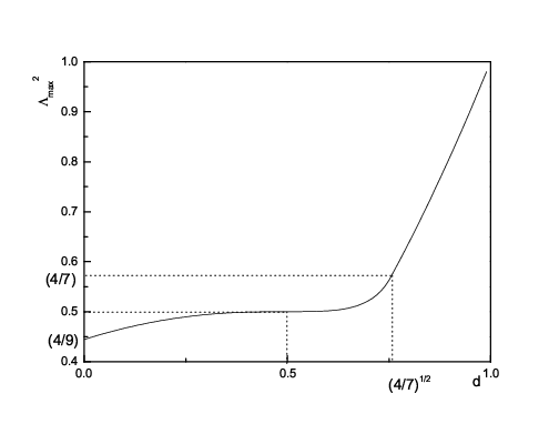
We have distinguished three types of quantum states depending on which expression takes entanglement eigenvalue. Also there are states that lie on surfaces separating different applicable domains. They are shared by two types of quantum states and may have interesting features. We will call those shared states. Such shared states are considered in the next section.

VI Shared States.

Consider quantum states for which both convex and crossed quadrangles yield the same entanglement eigenvalue. Eq.(36) is not applicable and we rewrite equations (27) and (35) as follows

4R_{q}^{2}=\frac{1}{2}\left(1-\frac{r}{16S^{2}_{q}}\right),\quad 4R_{\times}^{2}=\frac{1}{2}\left(1-\frac{r}{16S^{2}_{\times}}\right).

(59)

These equations show that if the state lies on the separating surface $r=0$ , then entanglement eigenvalue is a constant

\Lambda_{\max}^{2}=\frac{1}{2}

(60)

and does not depend on the state parameters. This fact has a simple interpretation. Consider the case $r_{1}=0$ . Then $b^{2}+c^{2}=a^{2}+d^{2}=1/2$ and the quadrangle consists of two right triangles. These two triangles have a common hypotenuse and legs $b,c$ and $a,d$ , respectively, regardless of the triangles being in the same semicircle or in opposite semicircles. In both cases they yield same circumradius. Decisive factor is that the center of the circumcircle lies on the diagonal. Thus the perimeter and diagonals of the quadrangle divide ranges of definition of the convex quadrangle. When the center of circumcircle passes the perimeter, entanglement eigenvalue changes-over from convex circumradius to the largest coefficient. And if the center lies on the diagonal, convex and crossed circumradiuses become equal.

We would like to bring plausible arguments that this picture is incomplete and there is a region that has been shrunk to the point. Consider three-qubit state given by GSD

|\psi\rangle=a|100\rangle+b|010\rangle+b|001\rangle+d|111\rangle+e|000\rangle.

(61)

One of parameters must have non-vanishing phase[10] and we can treat this phase as an angle. Then, we have five sides and an angle. This set defines a sexangle that has circumcircle. One can guess that in a highly entangled region entanglement eigenvalue is the circumradius of the sexangle. However, there is a crucial difference. Any convex sexangle contains a star type area and the sides of this area are the diagonals of the sexangle. The perimeter of the star separates the convex and the crossed cases. Unfortunately, we can not see this picture in our case because the diagonals of a quadrangle confine a single point. It is left for future to calculate the entanglement eigenvalues for arbitrary three qubit states and justify this general picture.

Shared states given by $r=0$ acquire new properties. They can be used for perfect teleportation and superdense coding [25, 27, 28]. This statement is not proven clearly, but also no exceptions are known.

Now consider a case where the largest coefficient and circumradius of the convex quadrangle coincide with each other. The separating surface is given by

l^{2}=\frac{1}{2}+\frac{abcd}{l^{2}}.

(62)

Entanglement eigenvalue ranges within the narrow interval

\frac{1}{2}\leq\Lambda_{\max}^{2}\leq\frac{4}{7}.

(63)

It separates slightly and highly entangled states. When one of coefficients is large enough and satisfies the relation $l^{2}>1/2+abcd/l^{2}$ , entanglement eigenvalue takes a larger coefficient. And the expression (8) for the state function effectively takes the place of Schmidt decomposition. In highly entangled region no similar picture exists and all coefficients participate in equal parts and yield the circumradius. Thus, shared states given by Eq.(62) separate slightly entangled states from highly entangled ones, and can be ascribed to both types.

What is the meaning of these states? Shared states given by $r=0$ acquire new and important features. One can expect that shared states dividing highly and slightly entangled states also must acquire some new features. However, these features are yet to be discovered.

VII Conclusions

We have considered three-parametric families of three qubit states and derived explicit expressions for entanglement eigenvalue. The final expressions have their own geometrical interpretation. The result in this paper with the results of Ref.[25] show that the geometric measure has two visiting cards: the circumradius and the largest coefficient. The geometric interpretation may enable us to predict the answer for the states given by GSD. If the center of circumcircle lies in star type area confined by diagonals of the sexangle, then entanglement eigenvalue is the circumradius of the crossed sexangle(s). If the center lies in the remaining part of sexangle, the entanglement eigenvalue is the circumradius of the convex sexangle. And when the center passes the perimeter, then entanglement eigenvalue is the largest coefficient. Although we cannot justify our prediction due to lack of computational technique, this picture surely enables us to take a step toward a deeper understanding of the entanglement measure [29].

Shared states given by $r=0$ play an important role in quantum information theory. The application of shared states given by Eq.(62) is somewhat questionable, and should be analyzed further. It should be pointed out that one has to understand the properties of these states and find the possible applications. We would like to investigate this issue elsewhere.

Finally following our procedure, one can obtain the nearest product state of a given three-parametric W-type state. These two states will always be separated by a line of densities composed of the convex combination of W-type states and the nearest product states [30]. There is a separable density matrix $\varrho_{0}$ which splits the line into two parts as follows. One part consists of separable densities and another part consists of non-separable densities. It was shown in Ref.[30] that an operator $W=\varrho_{0}-\rho^{ABC}-\mathrm{tr}[\varrho_{0}(\varrho_{0}-\rho^{ABC})]I$ has the properties $\mathrm{tr}(W\rho^{ABC})<0$ , and $\mathrm{tr}(W\varrho)\geq 0$ for the arbitrary separable state $\varrho$ . The operator $W$ is clearly Hermitian and thus is an entanglement witness for the state. Thus our results allow oneself to construct the entanglement witnesses for W-type three qubit states. However, the explicit derivation of $\varrho_{0}$ seems to be highly non-trivial [31, 32].

Acknowledgements.

LT thanks Edward Chubaryan for help. This work was supported by the Kyungnam University Research Fund, 2007.

References

[1] C. H. Bennett, H. J. Bernstein, S. Popescu, and B. Schumacher, Phys. Rev. A 53, 2046(1996).
[2] C. H. Bennett, D. P. DiVincenzo, J. A. Smolin, and W. K. Wootters, Phys. Rev. A 54, 3824(1996).
[3] V. Vedral, M. B. Plenio, M. A. Rippin, and P. L. Knight, Phys. Rev. Lett. 78, 2275(1997).
[4] M. B. Plenio and V. Vedral, J. Phys. A 34, 6997(2001).
[5] J. Eisert and H. J. Briegel, Phys. Rev. A 64, 022306(2001).
[6] D. A. Meyer and N. R. Wallach, J. Math. Phys. 43, 4273(2002).
[7] T.-C. Wei and P. M. Goldbart, Phys. Rev. A 68, 042307(2003).
[8] A. Shimony, Ann. NY. Acad. Sci 755, 675(1995).
[9] H. Barnum and N. Linden, J. Phys. A: Math. Gen. 34, 6787(2001).
[10] A. Acín, A. Andrianov, L. Costa, E. Jané, J. I. Latorre, and R. Tarrach, Phys. Rev. Lett. 85, 1560(2000).
[11] D. Greenberger, M. Horne, and A. Zeilinger, arXiv:0712.0921[quant-ph].
[12] W. Dür, G. Vidal and J. I. Cirac, Phys.Rev. A 62, 062314(2000).
[13] O. Biham, M. A. Nielsen and T. J. Osborne, Phys. Rev. A 65, 062312(2002).
[14] D. Shapira, Y. Shimoni, and O. Biham, Phys. Rev. A 73, 044301(2006).
[15] L. K. Grover, Phys. Rev. Lett. 79, 325(1997).
[16] R. Werner and A. Holevo, J. Math. Phys. 43, 4353(2002).
[17] T.-C. Wei, M. Ericsson, P. M. Goldbart and W. J. Munro, Quant. Inf. Comp. 4, 252(2004).
[18] D. Cavalcanti, Phys. Rev. A 73, 044302(2006).
[19] T.-C. Wei, J. B. Altepeter, P. M. Goldbart, and W. J. Munro, Phys. Rev. A 70, 022322(2004).
[20] A. B. Zamolodchikov, JETP Lett. 43 730(1986).
[21] R. Orús, Phys. Rev. Lett. 100, 130502(2008)
[22] Y. Cao and A. M. Wang, J. Phys. A: Math. Theor. 40, 3507(2007).
[23] D. Ostapchuk, G. Passante, R. Kobes, and G. Kunstatter, arXiv:0707.4020v2[quant-ph].
[24] E. Jung, M.-R. Hwang, H. Kim, M.-S. Kim, D.K. Park, J.-W. Son, and S. Tamaryan, Phys. Rev. A 77, 062317(2008).
[25] L. Tamaryan, D. K. Park, and S. Tamaryan, Phys. Rev. A 77, 022325(2008).
[26] Y. Shimoni, D. Shapira and O. Biham, Phys. Rev. A 69, 062303(2004).
[27] P. Agrawal and A. Pati, Phys. Rev. A 74, 062320(2006).
[28] E. Jung, M.-R. Hwang, D.K. Park, J.-W. Son, and S. Tamaryan, arXiv:0711.3520v1[quant-ph].
[29] E. Jung, M.-R. Hwang, D.K. Park, L. Tamaryan, and S. Tamaryan, Quant.Inf.Comp 8, 925(2008), arXiv:0803.3311v2[quant-ph].
[30] A. O. Pittenger and M. H. Rubin, Phys. Rev. A 67, 012327(2003).
[31] J. Sperling and W. Vogel, arXiv:0805.1318v1 [quant-ph].
[32] Ph. Krammer, arXiv:0807.4830v1 [quant-ph].