A simple cubic interaction of a charged scalar $\phi$ and a neutral $\chi$ scalar in a two-dimensional theory is considered,

$$\mathcal{L}=\frac{1}{2}|D_{\mu}\phi|^{2}-\frac{1}{2}\mu^{2}|\phi|^{2}+\frac{1}{2}(\partial_{\mu}\chi)^{2}-\frac{1}{2}m^{2}\chi^{2}+\lambda\,\phi\phi^{*}\chi,$$

(1)

where the covariant derivative given as $D_{\mu}=\partial_{\mu}+ieA_{\mu}$. The masses of the fields being $\mu$ and $m$ are first kept arbitrary, but after proceding to the semiclassical approximation it will be assumed that $\frac{m}{\mu}\ll 1$. This situation is known in vacuum decay terms as “an almost spherical bubble” and is used, e.g. in [14]. The charged field interacts with an external Abelian field $A_{\mu}$.

One can show  [18] that in the coordinate representation a free Green function at zero temperature for a particle of field $\chi$ with zero charge is

$$G_{\chi}(x,y)=\frac{1}{(4\pi)^{2}}\int_{0}^{\infty}\frac{d\alpha}{\alpha}\,\mathrm{e}^{\scriptstyle im^{2}\alpha\textstyle-\frac{i(y-x)^{2}}{4\alpha}},$$

(2)

where we have omitted the pole prescription $i\varepsilon$. For the charged particle $\phi$ in the constant external field $A_{\mu}=(0,Ex_{0})$ it becomes

$$G_{\phi}(x,y)=\frac{1}{(4\pi)^{2}}\int_{0}^{\infty}\frac{\epsilon d\alpha}{\sinh(\epsilon\alpha)}\,\mathrm{e}^{\scriptstyle im^{2}\alpha\textstyle-\frac{i\epsilon}{4}\scriptstyle(y-x)^{2}\coth(\epsilon\alpha)-\textstyle\frac{i\epsilon}{4}\scriptstyle(y_{1}-x_{1})(y_{0}+x_{0})},$$

(3)

where $\epsilon=eE$; the field is considered to be far below the Schwinger limit $\frac{m^{2}}{\epsilon}\gg 1$. We shall refer to representation (3) as Schwinger parametrization, and the variable $\alpha$ — Schwinger parameter. When the temperature is not equal to zero, the Green function is periodic in the Euclidean time with a period $\beta\equiv\frac{1}{T}$, hence [11] its generalization is organized as

$$\begin{array}[]{lll}G_{\phi}(x,y)&=&\displaystyle\sum_{n}\int^{\infty}_{0}\frac{\epsilon\,d\alpha}{(4\pi)^{2}\sinh(\epsilon\alpha)}\,\mathrm{e}^{\scriptstyle im^{2}\alpha\textstyle-\frac{i\epsilon}{4}\scriptstyle\left[(y_{0}-x_{0}+n\beta)^{2}+(y_{1}-x_{1})^{2}\right]\coth(\epsilon\alpha)}\times\\ &\times&\mathrm{e}^{-\textstyle\frac{i\epsilon}{4}\scriptstyle(y_{1}-x_{1})(y_{0}+x_{0}+n\beta)}.\end{array}$$

(4)

The sum over $n$ naturally appears since one should take into account all the equivalent positions separated by $\beta$ in Euclidean time, as explained in the cited paper.

Let us consider the one-loop perturbative correction to the Green function of the uncharged particle due to the cubic interaction mentioned above

$$\delta G_{\chi}(0,z)=\lambda^{2}\int d^{2}xd^{2}yG_{\chi}(0,x)G_{\phi}(x,y)G_{\phi}(y,x)G_{\chi}(y,z).$$

(5)

We think of a one-loop diagram, represented in configuration space in Figure 1.

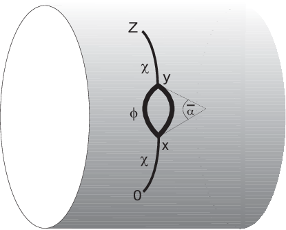
We stress here that our adherence to configuration space representation of vacuum polarization is not an incidental or technical detail of calculation, but is rather of conceptual meaning. Namely, as we have shown in our previous paper  [7], the saddle-point values of $\alpha_{i}$ correspond directly to the geometric parameters of the classical sub-barrier (Euclidean) trajectory in configuration space. The other reason to keep the position space is the direct relationship of the spatial configuration shown in Figure 1 to a vacuum bubble with external lines attached to it [14] describing induced vacuum decay on a compactified manifold.

The correction to Green function of the neutral $\chi$ field becomes then

$$\begin{array}[]{lll}\displaystyle\delta G_{\chi}(0,z)&=&\displaystyle\frac{\lambda^{2}\epsilon^{2}}{(4\pi)^{8}}\sum_{p,q,k,n}\int^{\infty}_{0}\frac{d\alpha_{1}\,d\alpha_{2}\,d\alpha_{3}\,d\alpha_{4}\,d^{2}x\,d^{2}y}{\sinh(\epsilon\alpha_{1})\sinh(\epsilon\alpha_{2})\,\alpha_{3}\,\alpha_{4}}\,\mathrm{e}^{\scriptstyle i\mu^{2}(\alpha_{1}+\alpha_{2})+im^{2}(\alpha_{3}+\alpha_{4})}\times\\ &\times&\mathrm{e}^{\textstyle-\frac{i(x_{0}+k\beta)^{2}}{4\alpha_{3}}-\frac{i(z_{0}-y_{0}+n\beta)^{2}}{4\alpha_{4}}-\textstyle\frac{ix_{1}^{2}}{4\alpha_{3}}-\frac{i(z_{1}-y_{1})^{2}}{4\alpha_{4}}+\textstyle\frac{i\epsilon\beta}{2}\scriptstyle(y_{1}-x_{1})(p-q)}\\ &\times&\mathrm{e}^{\textstyle-\frac{i\epsilon}{4}\scriptstyle[(y_{0}-x_{0}+p\beta)^{2}+(y_{1}-x_{1})^{2}]\coth(\epsilon\alpha_{1})\textstyle-\frac{i\epsilon}{4}\scriptstyle[(y_{0}-x_{0}+q\beta)^{2}+(y_{1}-x_{1})^{2}]\coth(\epsilon\alpha_{2})}.\end{array}$$

(6)

Note that due to temperature, Lorentz-invariance is explicitly broken in this expression. We may relate coordinate representation of the Green function correction to

$$\delta G(n,k_{1})=\int\delta G(0;z_{0},z_{1})\,\mathrm{e}^{-i\omega_{n}z_{0}-ik_{1}z_{1}}\,dz_{0}\,dz_{1},$$

(7)

where $\omega_{n}=\frac{2\pi n}{\beta}$. Calculation of this correction corresponds, as usually, to the shift of the Green’s function pole

$$G(n,\vec{k})=\frac{i}{\omega_{n}^{2}+k_{1}^{2}+m^{2}+M^{2}(n,k_{1})},$$

(8)

however, now the shift is not Lorentz-invariant but rather depends on both $n$ and $\vec{k}$ separately. Whatever complicated expression for the variation of the Green function one would obtain, physically relevant information is contained in the pole shift and rescaling of the wave function. Further on, only the pole shift will be considered. The mass shift is the value of the $M^{2}$ calculated at the point corresponding to the pole. For the zero temperature theory that means that the shift is determined only by the value of bare mass (and a scale). Since in this case $M^{2}(k^{2})$ depends only on $k^{2}=k_{0}^{2}-k_{1}^{2}$, one should take $k^{2}=m^{2}$. For a theory in a compactified Euclidean space-time it is quite obvious that the shift should depend on $n$ as $M^{2}(n,k_{1})$, where $n$ and $k_{1}$ such that $\omega_{n}^{2}+k_{1}^{2}+m^{2}=0$. For the $n$-th Matsubara mode the pole shift is approximately related to a Green function variation as

$$\delta m^{2}_{n}=-\left[\left(m^{2}+k_{1}^{2}+\frac{4\pi^{2}n^{2}}{\beta^{2}}\right)^{2}\delta G(k_{1},n)\right]_{\omega_{n}^{2}+\vec{k}^{2}+m^{2}=0}.$$

(9)

Moreover the on-shell condition does not have a solution for arbitrary $k_{1}^{2}$ since $\omega_{n}$ is determined by the discrete variable $n$. Note again that generically every single mode is renormalized in its own way. One can easily understand that due to Lorentz symmetry violation by compactifying the Euclidean time direction there is no invariant mass anymore. Rather, if some physical quantities related to thermal theory are of interest, the partition function $Z(\beta,\mu,\dots)$ has to be calculated, at some values of chemical potential $\mu$ and other external potentials. Then some statistically averaged reasonable quantities have to be found¹¹ 1 The authors are extremely grateful to Professor H. M. Kleinert for a discussion on this point., say, $n_{i}=\frac{\partial Z}{\partial\mu_{i}}$, which is the equilibrium concentration of particles of the $i$-th type.

Therefore, (9) is understood merely as a convenient way of writing down the propagator variation. However, there is a range of parameters within which it is still possible to preserve the meaning of this quantity as the mass shift of the particle. This range is the limit of small temperatures or large $\beta$. In this case on-shell condition can be solved even for $k_{1}=0$, since for sufficiently large $\beta$ the value of $\frac{m\beta}{2\pi}$ differs from an integer slightly. So one can treat the imaginary part of the mass shift for such $n$ and $k_{1}=0$ as the decay rate of the particle in the external field with a temperature not equal to zero.

Evaluating elementary integrals, one gets a formal expression for the mass shift

$$\displaystyle\begin{array}[]{lll}\displaystyle\delta m^{2}&=&\displaystyle\frac{\lambda^{2}}{\beta\,\epsilon^{3/2}}\sum\limits_{r,s\in\mathbb{Z}}\delta_{n+r+s}\int\limits^{+\infty+i0}_{0}\frac{d\alpha_{1}d\alpha_{2}}{\sqrt{\sinh(\alpha_{1}+\alpha_{2})\cosh(\alpha_{1}-\alpha_{2})}}\\ &\times&\displaystyle\mathrm{e}^{\textstyle\frac{4\pi^{2}i}{\epsilon\beta}\frac{(r\tanh(\alpha_{1})-s\tanh(\alpha_{2}))^{2}\sinh(2\alpha_{1})\sinh(2\alpha_{2})}{4\sinh(\alpha_{1}+\alpha_{2})\cosh(\alpha_{1}-\alpha_{2})}}\times\\ &\times&e^{\scriptstyle i\left[r^{2}\tanh(\alpha_{1})+s^{2}\tanh(\alpha_{2})\textstyle+\frac{\mu^{2}}{\epsilon}\scriptstyle(\alpha_{1}+\alpha_{2})\textstyle+\frac{4\pi^{2}n^{2}}{\epsilon\beta^{2}}\frac{1}{\coth(\alpha_{1})+\coth(\alpha_{2})}\right]}.\end{array}$$

(10)

By using the approximate on-shell condition $n\approx\frac{\mu\beta}{2\pi}$ and Poisson resummation formula

$$\sum_{n=-\infty}^{\infty}f(n)=\sum_{n=-\infty}^{\infty}\tilde{f}(2\pi n)$$

where

$$\tilde{f}(k)=\int^{\infty}_{-\infty}f(t)e^{-ikt}dt,$$

this expression can be written down in two equivalent representations. Now and further we retain its imaginary part solely, rather then the full (possibly divergent) pole shift in the propagator. These two representations are

$$\Gamma=\mathrm{Im}\frac{\lambda^{2}}{m\beta\,\epsilon^{3/2}}\sum_{s=-\infty}^{+\infty}\int\frac{d\alpha_{1}\,d\alpha_{2}\,\mathrm{e}^{\textstyle\frac{i\mu^{2}}{\epsilon}\scriptstyle(\alpha_{1}+\alpha_{2})\textstyle-\frac{im^{2}}{\epsilon}\frac{1}{\coth(\alpha_{1})+\coth(\alpha_{2})}+{\frac{4i\pi^{2}A}{\epsilon\beta^{2}}\scriptstyle(s-s_{0})^{2}}}}{\sqrt{\sinh(\alpha_{1}+\alpha_{2})\,\cosh(\alpha_{1}-\alpha_{2})}}$$

(11)

and

$$\Gamma=\mathrm{Im}\frac{\lambda^{2}}{m\epsilon}\sum_{s=-\infty}^{+\infty}\int\frac{d\alpha_{1}\,d\alpha_{2}\,\mathrm{e}^{\textstyle\frac{i\mu^{2}}{\epsilon}\scriptstyle(\alpha_{1}+\alpha_{2})\textstyle-\frac{im^{2}}{\epsilon}\frac{1}{\coth(\alpha_{1})+\coth(\alpha_{2})}\textstyle-\frac{i\epsilon\beta^{2}s^{2}}{4A}\scriptstyle-2\pi iss_{0}}}{\sinh(\alpha_{1}+\alpha_{2})},$$

(12)

where

$$A=\frac{\sinh(\alpha_{1}+\alpha_{2})}{\cosh(\alpha_{1}-\alpha_{2})},$$

$$s_{0}=\frac{m\beta}{2\pi}\frac{1}{\tanh(\alpha_{2})\coth(\alpha_{1})+1}.$$

The sums above can formally be converted to Jacobi theta-functions, however, that would not be of much use, since the integrals over Schwinger parameters would then get out of feasibility. On the contrary, one can do the integrals in Schwinger parameters by saddle-point method for each term in the sum, provided saddle-point works at all. Then in principle one could try to do the sum exactly.

When dealing in such way with 1-dimensional saddle-point integrals

$$\int dz\sum_{n}\mathrm{e}^{if_{n}(z)}$$

it will be necessary to restrict the domain of applicability of this approximation by imposing the conditions in saddle-point values $z=\bar{z}_{n}$ for the $n$th function $f_{n}$  [19]:

	$\displaystyle\displaystyle|f_{0}^{\prime\prime}(\bar{z}_{0})|^{3/2}\gg|f_{0}^{\prime\prime\prime}(\bar{z}_{1})|,$		(13)
	$\displaystyle|f_{1}^{\prime\prime}(\bar{z}_{0})|^{3/2}\gg f_{1}^{\prime\prime\prime}(\bar{z}_{1}),$		(14)
	$\displaystyle\mathrm{Im}[f_{0}(\bar{z_{0}})]\gg\mathrm{Im}[f_{1}(\bar{z}_{1})].$		(15)

Condition (13) ensures the possibility of doing saddle-point approximation for the zero mode. It checks whether the next-to-leading order terms in the decomposition of $f_{0}$ may be neglected. Condition (14) provides the same check for the first mode. To ensure dominance of the zero mode over the first one, we impose (15).

For multi-dimensional expressions the criteria of saddle-point method applicability become more complicated. Namely, instead of (13) or (14) one must require that

$$\frac{\partial^{3}f}{\partial z_{i}\partial z_{j}\partial z_{k}}P_{il}P_{jm}P_{kn}\frac{1}{\sqrt{\lambda_{l}\lambda_{m}\lambda_{n}}}\ll 1$$

(16)

where $\lambda_{i}$ are eigenvalues of second derivatives matrix $\frac{\partial^{2}f}{\partial z_{i}\partial z_{j}}$, and $P_{ij}$ is diagonalisation matrix for $\frac{\partial^{2}f}{\partial z_{i}\partial z_{j}}$, summation implied over $i,j,k,l,m,n$. Further it will be examined whether these conditions are satisfied for a particular saddle-point function under consideration.

The expression (12) seems to be an appropriate representation for the $\Gamma$ in the case $\beta\to\infty$, since even the naive condition of the saddle point method applicability fails for  (11), namely the factor in the exponent $\frac{1}{\epsilon\beta^{2}}$ becomes small. So, let us take  (12) and make sure that it indeed corresponds to the low-temperature limit. It is supposed that the saddle-point is a symmetric point $\alpha_{1}=\alpha_{2}=\alpha$. This is possible due to having particles of identical mass in the internal lines. Since the saddle-point values of Schwinger proper times, as shown in [7], correspond to the geometric parameters of the classical Euclidean loop configuration, only a symmetric configuration is expected to be the physically relevant solution of saddle-point equations.

The full “decay width” is a sum over Matsubara contributions

$$\Gamma=\sum_{n=-\infty}^{\infty}\Gamma_{n}.$$

It is expected that the higher the mode, the more suppressed it is. It will be shown below by means of saddle-point integral that this is indeed true for the zeroth and first modes. One can trivially see that the zero Matsubara mode exponential is

$$f_{0}=\frac{\mu^{2}}{\epsilon}2\alpha-\frac{m^{2}}{\epsilon}\frac{\tanh(\alpha)}{2},$$

identical to that of [7]. This function is extremized for $\alpha=\bar{\alpha}_{0}$ given by

$$\cosh(\bar{\alpha}_{0})=\frac{m}{2\mu}.$$

For simplicity the case of a very light external particle (“almost spherical bubble”) will be considered, that is $\frac{m}{\mu}\ll 1$. This is indeed the case of interest, as for a particle with $m>2\mu$ the process will become perturbatively allowed. Checking the conditions of saddle-point applicability (16), one gets

$$\frac{3}{\sqrt{2}\sqrt{\frac{m\mu}{\epsilon}}}\ll 1.$$

This condition is satisfied in our setting, due to having a sufficiently small field $\frac{m^{2}}{\epsilon}\gg 1$, imposed from the very beginning for the applicability of the saddle-point method (there always must be a significant exponential suppression). Thus the leading order (zero dual Matsubara mode) contribution to the sum (12) is

$$\Gamma_{0}\sim\frac{\pi}{\sqrt{\det_{i,j}\partial_{i}\partial_{j}f_{0}}}\,\mathrm{e}^{-f_{0}(\bar{\alpha})}.$$

In the leading order in both small parameters $\frac{m}{\mu}$ and $\frac{1}{\epsilon\beta^{2}}$ one obtains

$$\det_{i,j}\partial_{i}\partial_{j}f_{0}=\frac{4\mu^{4}}{\epsilon^{2}},$$

hence

$$\Gamma_{0}\sim\frac{\lambda^{2}}{m^{2}\mu}\,\mathrm{e}^{\textstyle-\frac{\pi\mu^{2}}{\epsilon}},$$

(17)

in agreement with [7]. The next-to-leading term is given by the modes with $s=\pm 1$. In the limit $\epsilon\beta^{2}\gg 1,\mu\gg m$ one obtains

$$f_{\pm 1}=\frac{\mu^{2}}{\epsilon}2\alpha-\frac{\epsilon\beta^{2}}{4\sinh 2\alpha}.$$

That amounts to the saddle-point equations

$$\cosh 2\alpha=\frac{4\mu^{2}}{\epsilon^{2}\beta^{2}},$$

solved by

$$\bar{\alpha}\approx\frac{\pi i}{4}$$

in the said approximation. Collecting all the terms, one gets the first correction

$$\Gamma_{\pm 1}\sim\frac{\lambda^{2}}{m\epsilon^{2}\beta^{2}}\,\mathrm{e}^{\textstyle-\frac{\epsilon\beta^{2}}{4}}.$$

(18)

It can be seen that the dependence on a temperature is essentially non-perturbative.

Upon calculating the second and the third derivatives of $f_{\pm 1}$, one gets the following inequality as the condition for saddle-point method applicability by evaluating (16)

$$\frac{16\mu^{2}}{\beta^{3}\epsilon^{5/2}}\ll 1,$$

(19)

which can be rewritten as

$$\beta\gg\frac{1}{\mu}\left(\frac{\mu^{2}}{\epsilon}\right)^{\frac{5}{6}}.$$

(20)

Obviously this condition is fulfilled provided that the temperature is high enough. The value of the exponential $f_{\pm 1}$ on the saddle point in the leading asymptotics is

$$f_{\pm 1}(\bar{\alpha}_{0})=\frac{i}{4}\beta^{2}\epsilon.$$

In the aforementioned limit the $s$-th mode will be suppressed like $e^{-\epsilon\beta^{2}s^{2}}$. The condition for the effective suppression roughly is

$$\beta\gg\frac{\mu}{\epsilon},$$

which is satisfied for $\beta\to\infty$ limit. Thus one makes sure that the chosen form of the series (12) indeed suites low-temperature region description.

Naively, it seems that one can easily perform similar calculations for the opposite case of extremely high temperatures. Just using the dual representation for the decay rate  (11) and applying the saddle point method one could get the answer. However, this is not necessarily so for several reasons. In both representations for $\Gamma$ the pole has already been chosen by setting $k_{1}^{2}=0$. It is easy to see that it is impossible to set $k_{1}^{2}=0$ and find such an integer value $n$ which would satisfy the on-shell condition $\frac{4\pi^{2}n^{2}}{\beta^{2}}+m^{2}=0$ for small $\beta$. So, in order to fulfill the on-shell condition and, thus, to find the proper expression for the rate in the limit of high temperature, one should keep $\vec{k}^{2}$ non-zero, which reflects violation of Lorentz symmetry by introducing a temperature. It is also worth mentioning that in this case, since one cannot get rid of the dependence on $n$, it is absolutely necessary to consider the renormalization for each Matsubara mode separately. The result certainly cannot be interpreted then as a high temperature decay rate of the initial particle. It is just some correction to the Green function, the physical meaning of which is not well defined. It may be meaningful in a compactified theory rather than in a thermal one. Intuitively one expects that at high temperatures tunneling term $e^{-S_{0}}$ (instanton contribution to the semiclassical expression) will be dominated over by the over-barrier term $e^{-\beta E}$(“sphaleron” contribution). However, in the saddle-point analysis performed by us, the “sphaleron” term has not appeared in the limit $\beta\to 0$. Thus no final judgement is passed on the applicability of saddle-point method at $\beta\to 0$, but it is doubtful that it can work as directly as it has worked for $\beta\to\infty$.

The values of $\bar{\alpha}$ given above are, of course, not unique. The true solution to the saddle-point equation is a series of roots like, say, $\bar{\alpha}=\pm i\arccos\frac{m}{2\mu}+2\pi in,\quad n\in\mathbb{Z}$. Therefore, an additional resummation to include all these roots is to be performed in principle. It is not necessary from a practical point of view, the terms in the series being suppressed by the factor $e^{-\frac{\mu^{2}}{\epsilon}}$, however, this resummation is noted in order to stress the similarity of the saddle-point configuration, on which the 1-loop integral is essentially calculated, and the world-line instanton configuration, proposed in the semiclassical approach by Dunne et al. [15, 16].

References

- [1] W. Heisenberg and H. Euler, Z. Phys. 98 (1936) 714 [arXiv:physics/0605038].
- [2] A. S. Gorsky, K. A. Saraikin and K. G. Selivanov, Nucl. Phys. B 628 (2002) 270 [arXiv:hep-th/0110178].
- [3] I. Y. Kobzarev, L. B. Okun and M. B. Voloshin, Sov. J. Nucl. Phys. 20, 644 (1975) [Yad. Fiz. 20, 1229 (1974)].
- [4] S. R. Coleman, Phys. Rev. D 15, 2929 (1977) [Erratum-ibid. D 16, 1248 (1977)].
- [5] I. K. Affleck and F. De Luccia, Phys. Rev. D 20, 3168 (1979).
- [6] K. Selivanov and M. Voloshin, ZHETP Lett,42 (1985) 422.
- [7] A. K. Monin and A. V. Zayakin, Phys. Rev. D 75, 065029 (2007) [arXiv:hep-th/0611038].
- [8] W. Dittrich, Phys. Rev. D 19, 2385 (1979).
- [9] M. Loewe and J. C. Rojas, Phys. Rev. D 46, 2689 (1992).
- [10] P. Elmfors, D. Persson and B. S. Skagerstam, Phys. Rev. Lett. 71, 480 (1993) [arXiv:hep-th/9305004].
- [11] H. Gies, Phys. Rev. D 60, 105002 (1999) [arXiv:hep-ph/9812436].
- [12] H. Gies, Phys. Rev. D 61, 085021 (2000) [arXiv:hep-ph/9909500].
- [13] J. Garriga, Phys. Rev. D 49, 5497 (1994) [arXiv:hep-th/9401020].
- [14] A. Gorsky and M. B. Voloshin, Phys. Rev. D 73, 025015 (2006) [arXiv:hep-th/0511095].
- [15] G. V. Dunne and C. Schubert, Phys. Rev. D 72, 105004 (2005) [arXiv:hep-th/0507174].
- [16] G. V. Dunne, Q. H. Wang, H. Gies and C. Schubert, Phys. Rev. D 73, 065028 (2006) [arXiv:hep-th/0602176].
- [17] Popov V. S., Marinov M. S. E+ E- Pair Production In Variable Electric Field Yad. Fiz. 16, 809 (1972).
- [18] J. S. Schwinger, Phys. Rev. 82, 664 (1951).
- [19] M. V. Fedoryuk. Saddle-Point Method. (Metod Perevala, in Russian), p.162. Moscow, “Nauka”, 1970, 362 pp.