The Determination of $\alpha_{\scriptscriptstyle S}$ from $\tau$ Decays Revisited

M. Davier S. Descotes-Genon A. Höcker B. Malaescu Z. Zhang Affiliation: Laboratoire de l’Accélérateur Linéaire, IN2P3/CNRS et Université Paris-Sud 11 (UMR 8607), F–91405, Orsay Cedex, France Affiliation: Laboratoire de Physique Théorique, CNRS et Université Paris-Sud 11 (UMR 8627), F–91405, Orsay Cedex, France Affiliation: CERN, CH–1211, Geneva 23, Switzerland

Abstract

We revisit the determination of $\alpha_{\scriptscriptstyle S}(m_{\tau}^{2})$ using a fit to inclusive $\tau$ hadronic spectral moments in light of (1) the recent calculation of the fourth-order perturbative coefficient $K_{4}$ in the expansion of the Adler function, (2) new precision measurements from BABAR of $e^{+}e^{-}$ annihilation cross sections, which decrease the uncertainty in the separation of vector and axial-vector spectral functions, and (3) improved results from BABAR and Belle on $\tau$ branching fractions involving kaons. We estimate that the fourth-order perturbative prediction reduces the theoretical uncertainty, introduced by the truncation of the series, by 20% with respect to earlier determinations. We discuss to some detail the perturbative prediction of two different methods: fixed-order perturbation theory (FOPT) and contour-improved perturbative theory (CIPT). The corresponding theoretical uncertainties are studied at the $\tau$ and $Z$ mass scales. The CIPT method is found to be more stable with respect to the missing higher order contributions and to renormalisation scale variations. It is also shown that FOPT suffers from convergence problems along the complex integration contour. Nonperturbative contributions extracted from the most inclusive fit are small, in agreement with earlier determinations. Systematic effects from quark-hadron duality violation are estimated with simple models and found to be within the quoted systematic errors. The fit based on CIPT gives $\alpha_{\scriptscriptstyle S}(m_{\tau}^{2})=0.344\pm 0.005\pm 0.007$ , where the first error is experimental and the second theoretical. After evolution to $M_{Z}$ we obtain $\alpha_{\scriptscriptstyle S}(M_{Z}^{2})=0.1212\pm 0.0005\pm 0.0008\pm 0.0005$ , where the errors are respectively experimental, theoretical and due to the evolution. The result is in agreement with the corresponding ${\rm N}^{3}{\rm LO}$ value derived from essentially the $Z$ width in the global electroweak fit. The $\alpha_{\scriptscriptstyle S}(M_{Z}^{2})$ determination from $\tau$ decays is the most precise one to date.

CERN-OPEN-2008-006, LAL 08-12, LPT-ORSAY 08-18, arXiv:0803.0979

August 24, 2026

1 Introduction

The relatively large mass of the $\tau$ lepton, its leptonic nature and its decay through weak interaction promotes it to a particular status for probing the Standard Model (see [1] for a detailed review, and references therein). In particular, spectral functions determined from the invariant mass distributions of hadronic $\tau$ decays are fundamental quantities describing the production of hadrons from the non-trivial vacuum of strong interactions. They embed similar information to the one determined from cross sections of $e^{+}e^{-}$ annihilation to hadrons: both kinds of spectral functions are especially useful at low energies where perturbative QCD fails to locally describe the data, and where the theoretical understanding of the strong interactions remains at a qualitative level. Due to these limitations on the theoretical side, spectral functions play a crucial role in calculations of hadronic vacuum polarisation contributions to observables such as the effective electromagnetic coupling at the $Z$ mass, and the muon anomalous magnetic moment.
Inclusive hadronic quantities, obtained after integrating over the spectral functions (or directly via the measurement of hadronic or leptonic $\tau$ branching fractions), have been found to be dominated by perturbative contributions at energies above $\sim$ 1 $\mathrm{\,Ge\kern-1.00006ptV}$ . They can be exploited to precisely determine the strong coupling constant at the $\tau$ -mass scale, $\alpha_{\scriptscriptstyle S}(m_{\tau}^{2})$ [2, 3, 4, 5]. More recently, this determination was reassessed [1] in the light of the existing data on $\tau$ decays and $e^{+}e^{-}$ annihilation.
In the present paper, we update the determination of $\alpha_{\scriptscriptstyle S}(m_{\tau}^{2})$ from hadronic $\tau$ decays, motivated by progress performed in two different areas: on the theoretical side, the perturbative expression of the relevant correlator has been computed up to fourth order [6], and on the experimental side, new precision measurements from BABAR of $\tau$ branching fractions involving kaons [7] decrease the uncertainty in the separation of vector and axial-vector spectral functions. We utilise this opportunity to analyse several features of the theoretical frameworks commonly used to determine $\alpha_{\scriptscriptstyle S}(m_{\tau}^{2})$ in more detail. This concerns the treatments of the perturbative series, the convergence of the expansions, and the impact of nonperturbative effects.
In Sec. 2 we describe recent experimental improvement on the measurements of $K\kern 1.99997pt\overline{\kern-1.99997ptK}{}\pi$ decays, the spectral functions and the $\tau$ branching fractions. This is followed in Sec. 3 by a summary of the various theoretical prescriptions used to extract $\alpha_{\scriptscriptstyle S}(m_{\tau}^{2})$ from a fit to data, and a discussion of their advantages and shortcomings. We also analyse the role played by nonperturbative contributions in this determination. In Sec. 4 we exploit the normalisation and shape of the spectral functions to constrain the relevant nonperturbative contributions and to provide an improved determination of $\alpha_{\scriptscriptstyle S}(m_{\tau}^{2})$ .

2 Tau Hadronic Spectral Functions

For vector (axial-vector) hadronic $\tau$ decay channels ${V^{-}}\nu_{\tau}$ ( ${A^{-}}\nu_{\tau}$ ), the nonstrange vector (axial-vector) spectral function $v_{1}$ ( $a_{1}$ , $a_{0}$ ), where the subscript refers to the spin $J$ of the hadronic system, is derived from the invariant mass-squared distribution $(1/N_{V/A})(dN_{V/A}/ds)$ for a given hadronic mass $\sqrt{s}$ , divided by the appropriate kinematic factor, and normalised to the hadronic branching fraction

v_{1}(s)/a_{1}(s)=\frac{m_{\tau}^{2}}{6\,|V_{ud}|^{2}\,S_{\rm EW}}\,\frac{{\cal B}_{V^{-}/A^{-}\nu_{\tau}}}{{\cal B}_{e}}\frac{dN_{V/A}}{N_{V/A}\,ds}\,\left[\left(1-\frac{s}{m_{\tau}^{2}}\right)^{\!\!2}\,\left(1+\frac{2s}{m_{\tau}^{2}}\right)\right]^{-1}\hskip-8.5359pt.

(1)

For $a_{0}(s)$ , the same expression holds if the term $(1+2s/m_{\tau}^{2})$ is removed. Here $S_{\rm EW}=1.0198\pm 0.0006$ is a short-distance electroweak correction [8, 9], ${\cal B}_{V^{-}/A^{-}\nu_{\tau}}$ ( ${\cal B}_{e}$ ) denotes the inclusive $\tau\to V^{-}/A^{-}(\gamma)\nu_{\tau}$ ( $\tau\to e^{-}\overline{\nu}_{e}\nu_{\tau}$ ) branching fraction (throughout this letter, final state photon radiation is accounted for in the $\tau$ branching fractions). We use universality in the leptonic weak charged currents and the measurements of ${\cal B}_{e}$ , ${\cal B}_{\mu}$ and the $\tau$ lifetime, to obtain the improved branching fraction ${\cal B}_{e}={\cal B}_{e}^{\rm uni}=(17.818\pm 0.032)\%$ [1]. We also use $m_{\tau}=(1776.90\pm 0.20)\mathrm{\,Me\kern-1.00006ptV}$ [10] and $|V_{ud}|=0.97418\pm 0.00019$ [11] (assuming CKM unitarity). Integration of the spectral function over the $\tau$ phase space leads to the inclusive $\tau$ hadronic width, expressed through the ratio

R_{\tau,V/A}=\frac{{\cal B}_{V^{-}/A^{-}\nu_{\tau}}}{{\cal B}_{e}}\,.

(2)

By unitarity and analyticity the spectral functions are connected to the imaginary part of the two-point correlation function, $\Pi_{ij,U}^{\mu\nu}(q)$ , for time-like momenta-squared $q^{2}>0$ ,

\Pi_{ij,U}^{\mu\nu}(q)\equiv i\int d^{4}x\,e^{iqx}\langle 0|T(U_{ij}^{\mu}(x)U_{ij}^{\nu}(0)^{\dagger})|0\rangle=\left(-g^{\mu\nu}q^{2}+q^{\mu}q^{\nu}\right)\,\Pi^{(1)}_{ij,U}(q^{2})+q^{\mu}q^{\nu}\,\Pi^{(0)}_{ij,U}(q^{2})\,,

(3)

where $U=A,V$ denotes the nature of the relevant currents, either vector $(U_{ij}^{\mu}=V_{ij}^{\mu}=\overline{q}_{j}\gamma^{\mu}q_{i})$ or axial-vector ( $U_{ij}^{\mu}=A_{ij}^{\mu}=\overline{q}_{j}\gamma^{\mu}\gamma_{5}q_{i}$ ) charged colour-singlet quark currents. By Lorentz decomposition, the correlation functions can be split into their $J=1$ and $J=0$ parts.
In the complex $s=q^{2}$ plane, the polarisation functions $\Pi_{ij,U}^{\mu\nu}(s)$ are expected to exhibit a very simple analytic structure, the only non-analytic features being along the real axis: a branch cut for all polarisation functions, and a pole at the pion (kaon) mass for $a_{0}$ . The imaginary part of the polarisation functions on the branch cut is linked to the spectral functions defined in Eq. (1), for nonstrange (strange) quark currents

{\rm Im}\Pi^{(1,0)}_{\overline{u}d(s),V/A}(s)=\frac{1}{2\pi}v_{1}/a_{1,0}(s)\>,

(4)

which provide the basis for comparing a theoretical description of strong interaction with hadronic data.
Experimentally, the total hadronic observable $R_{\tau}$ ,

R_{\tau}=R_{\tau,V}+R_{\tau,A}+R_{\tau,S}\>,

(5)

where $R_{\tau,S}$ denotes the hadronic width to final states with net strangeness, is obtained from the measured leptonic branching ratios,

R_{\tau}=\frac{1-{\cal B}_{e}-{\cal B}_{\mu}}{{\cal B}_{e}}=\frac{1}{{\cal B}_{e}^{\rm uni}}-1.9726=3.640\pm 0.010\>.

(6)

2.1 New Input to the Vector/Axial-Vector Separation

The separation of vector and axial-vector components is straightforward in the case of hadronic final states with only pions using $G$ -parity, provided that isospin symmetry holds. An even number of pions has $G=1$ corresponding to vector states, while an odd number of pions has $G=-1$ , which tags axial-vector states. Modes with a $K\kern 1.99997pt\overline{\kern-1.99997ptK}{}$ pair are not in general eigenstates of $G$ -parity and contribute to both $V$ and $A$ channels. While the decay to $K^{-}K^{0}$ is pure vector, additional information is required to separate the $K\kern 1.99997pt\overline{\kern-1.99997ptK}{}\pi$ and the rarer $K\kern 1.99997pt\overline{\kern-1.99997ptK}{}\pi\pi$ modes. For the latter channel an axial-vector fraction of $0.5\pm 0.5$ is used [1].
Until recently, there was some confusion on this issue for the $K\kern 1.99997pt\overline{\kern-1.99997ptK}{}\pi$ modes:

1.

In the ALEPH analysis of $\tau$ decay modes with kaons [12], an estimate of the vector contribution was obtained using the $e^{+}e^{-}$ annihilation data from DM1 [13] and DM2 [14] in the $K\kern 1.99997pt\overline{\kern-1.99997ptK}{}\pi$ channel, extracted in the $I=1$ state. This contribution was found to be small, and, using the conserved vector current (CVC), a branching fraction of ${\cal B}_{\rm CVC}(\tau\to\nu_{\tau}(K\kern 1.99997pt\overline{\kern-1.99997ptK}{}\pi)_{V})=(0.26\pm 0.39)\cdot 10^{-3}$ , was found, corresponding to an axial fraction of $f_{A,{\rm CVC}}(K\kern 1.99997pt\overline{\kern-1.99997ptK}{}\pi)=0.94^{+0.06}_{-0.08}$ .
2.

The ALEPH CVC result was corroborated by a partial-wave and lineshape analysis of the $a_{1}$ resonance from $\tau$ decays in the $\nu_{\tau}\pi^{-}2\pi^{0}$ mode performed by CLEO [15]. The effect of the $K^{\star}K$ decay mode of the $a_{1}$ was seen through unitarity and a branching fraction of ${\cal B}(a_{1}\to K^{\star}K)=(3.3\pm 0.5)\%$ was derived. With the known $\tau^{-}\to\nu_{\tau}a_{1}^{-}$ branching fraction, this value more than saturates the total branching fraction available for the $K\kern 1.99997pt\overline{\kern-1.99997ptK}{}\pi$ channel, yielding an axial fraction of $f_{A,a_{1}}(K\kern 1.99997pt\overline{\kern-1.99997ptK}{}\pi)=1.30\pm 0.24$ .
3.

Another piece of information, also contributed by CLEO [16], but conflicting with the two previous results, is based on a partial-wave analysis in the $K^{-}K^{+}\pi^{-}$ channel using two-body resonance production and including many possible contributing channels. A much smaller axial fraction of $f_{A,K\kern 1.63885pt\overline{\kern-1.63885ptK}{}\pi}(K\kern 1.99997pt\overline{\kern-1.99997ptK}{}\pi)=0.56\pm 0.10$ was found here.

Since the three determinations are inconsistent, the value $f_{A}=0.75\pm 0.25$ has been used previously to account for the discrepancy [1]. This led to a systematic uncertainty in the $V,A$ spectral functions that competed with the purely experimental uncertainties.
Precise cross section measurements for $e^{+}e^{-}$ annihilation to $K^{+}K^{-}\pi^{0}$ and to $K^{0}K^{\pm}\pi^{\mp}$ have been recently published by the BABAR Collaboration [7], using the method of radiative return. In the mass range of interest for $\tau$ physics they show strong dominance of $K^{\star}(890)K$ dynamics and a fit of the Dalitz plot yields a clean separation of the $I=0,1$ contributions. Assuming CVC, the mass distribution of the vector final state in the decays $\tau\to\nu_{\tau}K\kern 1.99997pt\overline{\kern-1.99997ptK}{}\pi$ can be obtained. The result is shown in Fig. 1 and compared with the full $\tau$ spectrum from ALEPH [12] summing up the contributions from the $K^{-}K^{+}\pi^{-}$ , $\kern 1.99997pt\overline{\kern-1.99997ptK}{}^{0}K^{0}\pi^{-}$ , and $K^{-}K^{0}\pi^{0}$ modes. The BABAR results reveal a small vector component. After integration, one obtains

f_{A,{\rm CVC}}(K\kern 1.99997pt\overline{\kern-1.99997ptK}{}\pi)=0.833\pm 0.024,

(7)

which is about $1.3\sigma$ lower than the ALEPH determination using the same method (but with much poorer $e^{+}e^{-}$ input data) and 2.7 $\sigma$ higher than the CLEO partial-wave-analysis result. The new determination has a precision that exceeds the previously used value by an order of magnitude, thus effectively reducing the uncertainties in the vector and axial-vector spectral functions to the experimental errors only.
One notices from Fig. 1 that the axial fraction varies versus the $K\kern 1.99997pt\overline{\kern-1.99997ptK}{}\pi$ mass, with lower masses being further axial-enhanced. The observed axial-vector dominance is at variance with several estimates such as $f_{A}\sim 0.10$ [17], 0.37 [18], obtained within the Resonance Chiral Theory, which attempts at incorporating massive vector and axial resonances decaying into light mesons into a framework inspired by chiral and large- $N_{c}$ arguments. On the other hand, this axial-vector dominance is closer to the prediction $f_{A}\sim 0.71$ , based on a model combining axial-vector and vector resonances of finite widths with a leading-order chiral Lagrangian [19].
In deriving Eq. (7) care was taken to include a small contribution from the $\phi\pi$ final state, observed by BABAR in the same analysis [7]. Since BABAR also published a $\tau^{-}\to\nu_{\tau}\phi\pi^{-}$ branching fraction measurement [20], it is possible to perform a test of CVC in this channel with

	$\displaystyle{\cal B}_{\rm CVC}(\tau\to\nu_{\tau}\phi\pi^{-})$	$\displaystyle=$	$\displaystyle(3.8\pm 0.9\pm 0.2)\cdot 10^{-5}\,,$		(8)
	$\displaystyle{\cal B}_{\tau}(\tau\to\nu_{\tau}\phi\pi^{-})$	$\displaystyle=$	$\displaystyle(3.42\pm 0.55\pm 0.25)\cdot 10^{-5}\,,$		(9)

for which we find agreement within the quoted statistical and systematic errors. For comparison the dominant CVC $\tau\to\nu_{\tau}K^{\star}(890)K$ branching fraction is $(7.3\pm 0.6\pm 0.4)\cdot 10^{-4}$ .

Refer to caption — Figure 1: The mass-squared distribution for $\tau\to\nu_{\tau}K\kern 1.99997pt\overline{\kern-1.99997ptK}{}\pi$ decay modes from ALEPH and the predictions for the vector component obtained by CVC using DM1, DM2 and BABAR $e^{+}e^{-}$ data.

2.2 Update on the Branching Fraction for Strange Decays

New measurements of $\tau$ strange decays have been published since our last compilation [1]. This is the case for the hadronic channels $K\pi^{0}$ [21], $K_{S}\pi^{-}$ [22], and $K^{-}\pi^{+}\pi^{-}$ [7]. Also using the more precise estimate from universality for the $K^{-}$ channel [1], the updated value of $R_{\tau,S}$ becomes

R_{\tau,S}=0.1615\pm 0.0040\>,

(10)

replacing the previous value of $0.1666\pm 0.0048$ [1].
Using the new $f_{A}(K\kern 1.99997pt\overline{\kern-1.99997ptK}{}\pi)$ value (7), the updated hadronic widths $R_{\tau,V/A}$ from ALEPH, slightly renormalised so that their sum agrees with the new average for $R_{\tau,V+A}$ obtained from (6) and (10) read

$\displaystyle R_{\tau,V}$	$\displaystyle=$	$\displaystyle 1.783\pm 0.011\pm 0.002\>,$	(11)
$\displaystyle R_{\tau,A}$	$\displaystyle=$	$\displaystyle 1.695\pm 0.011\pm 0.002\>,$	(12)
$\displaystyle R_{\tau,V+A}$	$\displaystyle=$	$\displaystyle 3.479\pm 0.011\>,$	(13)
$\displaystyle R_{\tau,V-A}$	$\displaystyle=$	$\displaystyle 0.087\pm 0.018\pm 0.003\>,$	(14)

where the first errors are experimental and the second due to the $V/A$ separation, now dominated by the $K\kern 1.99997pt\overline{\kern-1.99997ptK}{}\pi\pi$ channel.
The ALEPH spectral functions are updated accordingly and shown in Fig. 2 for respectively vector, axial-vector, $V+A$ and $V-A$ .

3 Theoretical Prediction of $R_{\tau}$

Tests of QCD and the precise measurement of the strong coupling constant $\alpha_{\scriptscriptstyle S}$ at the $\tau$ mass scale [2, 3, 4, 5], carried out first by the ALEPH [23] and CLEO [24] collaborations, have triggered many theoretical developments. They concern primarily the perturbative expansion for which different optimised rules have been suggested. Among these are contour-improved (resummed) fixed-order perturbation theory [26, 27], effective charge and minimal sensitivity schemes [28, 29, 30, 31, 32], the large- $\beta_{0}$ expansion [33, 34, 35], as well as combinations of these approaches. Their main differences lie in how they deal with the fact that the perturbative series is truncated at an order where the missing part is not expected to be small. While a review and discussion of the various approaches can be found in [1], we only recall some of their salient features in the following.
With the publication of the full vector and axial-vector spectral functions by ALEPH [36, 37] and OPAL [25] it became possible to directly study the nonperturbative properties of QCD through $V-A$ sum rules and through fits to spectral moments computed from weighted integrals over the spectral functions (we refer again to the discussions in [1]). Inclusive observables like $R_{\tau}$ can be accurately predicted in terms of $\alpha_{\scriptscriptstyle S}(m_{\tau}^{2})$ using perturbative QCD, and including small nonperturbative contributions within the framework of the Operator Product Expansion (OPE) [38].

3.1 Operator Product Expansion

According to Eq. (4), the absorptive (imaginary) parts of the vector and axial-vector two-point correlation functions $\Pi^{(J)}_{\overline{u}d,V/A}(s)$ , with the spin $J$ of the hadronic system, are proportional to the $\tau$ hadronic spectral functions with corresponding quantum numbers. The nonstrange ratio $R_{\tau,V+A}$ can be written as an integral of these spectral functions over the invariant mass-squared $s$ of the final state hadrons [4]

R_{\tau,V+A}(s_{0})=12\pi S_{\rm EW}|V_{ud}|^{2}\!\int\limits_{0}^{s_{0}}\frac{ds}{s_{0}}\left(1-\frac{s}{s_{0}}\right)^{\!\!2}\left[\left(1+2\frac{s}{s_{0}}\right){\rm Im}\Pi^{(1)}(s+i\varepsilon)\,+\,{\rm Im}\Pi^{(0)}(s+i\varepsilon)\right],\hskip 5.69046pt\mbox{}

(15)

where $\Pi^{(J)}$ can be decomposed as $\Pi^{(J)}=\Pi_{ud,V}^{(J)}+\Pi_{ud,A}^{(J)}$ . We work in the chiral limit¹¹ 1 Vector and axial-vector currents are conserved in the chiral limit, so that $s\Pi_{V}^{(0)}=s\Pi_{A}^{(0)}=0$ . to study the perturbative contribution, so that the lower integration limit is zero because of the pion pole at zero mass. The correlation function $\Pi^{(J)}$ is analytic in the complex $s$ plane everywhere except on the positive real axis where singularities exist. Hence by Cauchy’s theorem, the imaginary part of $\Pi^{(J)}$ is proportional to the discontinuity across the positive real axis, and the integral (15) can be replaced by a contour integral over $\Pi(s)$ running counter-clockwise around the circle from $s=s_{0}+i\varepsilon$ to $s=s_{0}-i\varepsilon$ .
The energy scale $s_{0}=m_{\tau}^{2}$ is large enough that contributions from nonperturbative effects are expected to be subdominant and the use of the Operator Product Expansion is appropriate. The latter is expected to yield relevant results in the deep Euclidean region where $s$ is large and negative, whereas the extension to other regions in the complex plane is questionable. Fortunately, in the case of $R_{\tau}$ , the kinematic factor $(1-s/s_{0})^{2}$ suppresses the contribution from the region near the positive real axis where $\Pi^{(J)}(s)$ has a branch cut and the validity of the OPE is doubtful due to large quark-hadron duality violations [39, 40].
The OPE of the vector and axial-vector ratio $R_{\tau,V/A}$ can be written as

R_{\tau,V/A}=\frac{3}{2}S_{\rm EW}|V_{ud}|^{2}\bigg(1+\delta^{(0)}+\delta^{\prime}_{\rm EW}+\delta^{(2,m_{q})}_{ud,V/A}+\hskip-2.84544pt\hskip-2.84544pt\sum_{D=4,6,\dots}\hskip-2.84544pt\hskip-2.84544pt\hskip-2.84544pt\hskip-2.84544pt\delta_{ud,V/A}^{(D)}\bigg)\>,

(16)

with the massless universal²² 2 In the chiral limit of vanishing quark masses the contributions from vector and axial-vector currents coincide to any given order of perturbation theory and the results are flavour independent. perturbative contribution $\delta^{(0)}$ , the residual non-logarithmic electroweak correction $\delta^{\prime}_{\rm EW}=0.0010$ [43] (cf. the discussion on radiative corrections in [1]), and the dimension $D=2$ perturbative contribution $\delta^{(2,m_{q})}_{ud,V/A}$ from massive quarks. The term $\delta^{(D)}$ denotes the OPE contributions of mass dimension $D$ [5]

\delta_{ud,V/A}^{(D)}=\hskip-2.84544pt\hskip-2.84544pt\hskip-2.84544pt\sum_{{\rm dim}{\cal O}=D}\hskip-2.84544pt\hskip-2.84544pt\hskip-2.84544ptC^{\prime}_{V/A}(s_{0},\mu)\frac{\langle{\cal O}_{D}(\mu)\rangle_{V/A}}{s_{0}^{D/2}}\>,

(17)

where $\delta_{ud,V+A}^{(D)}=\frac{1}{2}\big(\delta_{ud,V}^{(D)}+\delta_{ud,A}^{(D)}\big)$ . In practice, the OPE provides a separation between short and long distances by following the flow of a large incoming momentum. The scale parameter $\mu$ separates the long-distance nonperturbative effects, absorbed into the vacuum expectation value of the operators $\langle{\cal O}_{D}(\mu)\rangle$ , from the short-distance effects that are included in the coefficients $C_{V/A}(s,\mu)$ , which become $C^{\prime}_{V/A}(s_{0},\mu)$ after performing the integration (15). The vacuum expectation values $\langle{\cal O}_{D}(\mu)\rangle$ encode information on the nonperturbative features of QCD vacuum and its effects on the propagation of quarks: they cannot be computed from first principles and have to be extracted from data. The short-distance coefficients $C_{V/A}(s,\mu)$ can be determined within perturbative QCD.

3.2 Perturbative Contribution to Fourth Order in $\alpha_{\scriptscriptstyle S}$

$R_{\tau}$ is a doubly inclusive observable since it is the result of an integration over all hadronic final states at a given invariant mass and further over all masses between $m_{\pi}$ and $m_{\tau}$ . The scale $m_{\tau}$ lies in a compromise region where $\alpha_{\scriptscriptstyle S}(m_{\tau}^{2})$ is large enough so that $R_{\tau}$ is sensitive to its value, yet still small enough so that the perturbative expansion converges safely and nonperturbative power terms are small. The prediction for $R_{\tau}$ is thus found to be dominated by the lowest-dimension term in Eq. (17), i.e., the term obtained from a perturbative computation of the correlator $\Pi$ .
For the evaluation of the perturbative series, it is convenient to introduce the analytic Adler function [45] $D(s)\equiv-s\cdot d\Pi(s)/ds$ , which avoids extra subtractions that are unrelated to QCD dynamics. The function $D(s)$ calculated in perturbative QCD within the $\overline{\mathrm{MS}}$ renormalisation scheme is a function of $\alpha_{\scriptscriptstyle S}$ and depends on the renormalisation scale $\mu$ , occurring through $\ln(\mu^{2}/s)$ . Since $D(s)$ is connected to a physical quantity, the spectral function ${\rm Im}\Pi(s)$ , it cannot depend on the choice of the renormalisation scale $\mu$ . This is achieved through the cancellation of the $\mu$ -dependence of $\alpha_{\scriptscriptstyle S}$ and of the explicit occurrences of $\mu$ in $D$ . Nevertheless, in the realistic case of a series truncated at a given order in $\alpha_{\scriptscriptstyle S}$ our knowledge of the renormalisation scale dependence is imperfect, i.e., $D$ depends on $\mu$ , thus inducing a systematic uncertainty.
To introduce the Adler function in Eq. (15), one uses partial integration, giving

1+\delta^{(0)}=-2\pi i\hskip-2.84544pt\hskip-2.84544pt\oint\limits_{|s|=s_{0}}\hskip-2.84544pt\hskip-2.84544pt\frac{ds}{s}w(s)D(s)\>,

(18)

where $w(s)=1-2s/s_{0}+2(s/s_{0})^{3}-(s/s_{0})^{4}$ . The perturbative expansion of $D(s)$ reads

D(s)=\frac{1}{4\pi^{2}}\sum_{n=0}^{\infty}\tilde{K}_{n}(\xi)a_{s}^{n}(-\xi s)\>,

(19)

with $a_{s}\equiv\alpha_{\scriptscriptstyle S}/\pi$ , and where the dimensionless factor $\xi$ parametrises the renormalisation scale ambiguity. While the coefficients $K_{0,1}=\tilde{K}_{0,1}=1$ are universal (we use the notation $K_{n}=\tilde{K}_{n}(\xi=1)$ in the following), the $\tilde{K}_{n\geq 2}$ depend on the renormalisation scheme and scale used. Powerful computational techniques have recently allowed to determine $K_{4}$ . The authors of [6] exploited the dependence of the four-loop master integrals (used to express all relevant four-loop integrals with massless propagators) on the space-time dimension to compute the integrals to the required accuracy. For $n_{f}=3$ quark flavours and $\xi=1$ one has³³ 3 The numerical expressions for an arbitrary number of quark flavours ( $n_{f}$ ) in the $\overline{\mathrm{MS}}$ renormalisation scheme for $\xi=1$ are: $K_{0}=1$ , $K_{1}=1$ , $K_{2}\simeq 1.9857-0.1153\,n_{f}$ , $K_{3}\simeq 18.2428-4.2158\,n_{f}+0.0862\,n_{f}^{2}$ , and $K_{4}\simeq 135.7916-34.4402\,n_{f}+1.8753\,n_{f}^{2}-0.0101\,n_{f}^{3}$ . $K_{2}\simeq 1.640$ , $K_{3}\simeq 6.371$ and $K_{4}\simeq 49.08$ [46, 47, 48, 49, 50, 6]. The full expressions for the functions $\tilde{K}_{n}(\xi)$ for arbitrary $\xi$ up to order $n=5$ can be found in [1].
With the series (19), inserted into the r.h.s. of Eq. (18), one obtains the perturbative expansion

\delta^{(0)}=\sum_{n=1}^{\infty}\tilde{K}_{n}(\xi)A^{(n)}(a_{s})\>,

(20)

with the functions [26]

A^{(n)}(a_{s})=\frac{1}{2\pi i}\hskip-2.84544pt\oint\limits_{|s|=s_{0}}\hskip-2.84544pt\hskip-2.84544pt\frac{ds}{s}w(s)a_{s}^{n}(-\xi s)=\frac{1}{2\pi}\int\limits_{-\pi}^{\pi}d\varphi\,w(-s_{0}e^{i\varphi})a_{s}^{n}(\xi s_{0}e^{i\varphi})\,.

(21)

Similarly, the Adler function also serves to obtain the perturbative expansion of the inclusive $e^{+}e^{-}$ annihilation cross section ratio

R_{e^{+}e^{-}}(s)=\frac{\sigma(e^{+}e^{-}\to{\rm hadrons}\,(\gamma))}{\sigma(e^{+}e^{-}\to\mu^{+}\mu^{-})}=-6\pi i\sum_{f}Q_{f}^{2}\oint_{|s^{\prime}|=|s|}ds^{\prime}\cdot\frac{D(s^{\prime})}{s^{\prime}}.

(22)

Evaluating the contour integral in fixed-order perturbation theory (cf. Sec. 3.2.1) with $n_{f}=5$ active quark flavours, and inserting all known coefficients, gives⁴⁴ 4 The explicit formula reads: $\displaystyle R_{e^{+}e^{-}}(s)$ $\displaystyle=$ $\displaystyle 3\sum_{f}Q_{f}^{2}\bigg[1+a_{s}(s)+K_{2}\,a_{s}^{2}(s)+\left(K_{3}-\frac{1}{3}\pi^{2}\beta_{0}^{2}\right)a_{s}^{3}(s)+\left(K_{4}-\frac{5}{6}\pi^{2}\beta_{0}\beta_{1}-K_{2}\pi^{2}\beta_{0}^{2}\right)a_{s}^{4}(s)$ $\displaystyle\quad\quad\quad\quad+\left(K_{5}-\frac{1}{2}\pi^{2}\beta_{1}^{2}-\pi^{2}\beta_{0}\beta_{2}-\frac{7}{3}\pi^{2}\beta_{0}\beta_{1}K_{2}-2\pi^{2}\beta_{0}^{2}K_{3}\right.+\left.\frac{1}{5}\pi^{4}\beta_{0}^{4}\right)a_{s}^{5}(s)+\dots\bigg]\,.$

	$\displaystyle R_{e^{+}e^{-}}^{(5)}(s)$	$\displaystyle=$	$\displaystyle 3{\sum}_{f}Q_{f}^{2}\big[1+a_{s}(s)+1.4092\,a_{s}^{2}(s)-12.7673\,a_{s}^{3}(s)-79.9795\,a_{s}^{4}(s)$		(23)
			$\displaystyle\hskip 42.67912pt+\;(K_{5}+79.7306)\,a_{s}^{5}(s)+(K_{6}+2202.78)\,a_{s}^{6}(s)+\dots\big]\,.$		(23)

3.2.1 Fixed-Order and Contour-Improved Perturbation Theory

The standard perturbative method to compute the contour integral consists of expanding all the quantities up to a given power of $a_{s}(s_{0})$ . The starting point is the solution of the renormalisation group equation (RGE) for $a_{s}(s)$ , which is expanded in a Taylor series of $\eta\equiv\ln(s/s_{0})$ around the reference scale $s_{0}$ [1]

$\displaystyle a_{s}(s)$	$\displaystyle=$	$\displaystyle a_{s}-\beta_{0}\eta a_{s}^{2}+\left(-\beta_{1}\eta+\beta_{0}^{2}\eta^{2}\right)a_{s}^{3}+\bigg(-\beta_{2}\eta+\frac{5}{2}\beta_{0}\beta_{1}\eta^{2}-\beta_{0}^{3}\eta^{3}\bigg)a_{s}^{4}$	(24)
		$\displaystyle+\;\left(-\beta_{3}\eta+\frac{3}{2}\beta_{1}^{2}\eta^{2}+3\beta_{0}\beta_{2}\eta^{2}-\frac{13}{3}\beta_{0}^{2}\beta_{1}\eta^{3}+\beta_{0}^{4}\eta^{4}\right)a_{s}^{5}$
		$\displaystyle+\;\bigg(-\beta_{4}\eta+\frac{7}{2}\beta_{1}\beta_{2}\eta^{2}+\frac{7}{2}\beta_{0}\beta_{3}\eta^{2}-\frac{35}{6}\beta_{0}\beta_{1}^{2}\eta^{3}-6\beta_{0}^{2}\beta_{2}\eta^{3}+\frac{77}{12}\beta_{0}^{3}\beta_{1}\eta^{4}-\beta_{0}^{5}\eta^{5}\bigg)a_{s}^{6}+\mathcal{O}(\eta^{6};a_{s}^{7})~.$

Here the series has been reordered in powers of $a_{s}\equiv a_{s}(s_{0})$ and we use the RGE $\beta$ -function⁵⁵ 5 The full expressions for an arbitrary number of quark flavours ( $n_{f}$ ) are: $\beta_{0}=\frac{1}{4}\left(11-\frac{2}{3}n_{f}\right)$ , $\beta_{1}=\frac{1}{16}\left(102-\frac{38}{3}n_{f}\right)$ , $\beta_{2}=\frac{1}{64}\left(\frac{2857}{2}-\frac{5033}{18}n_{f}+\frac{325}{54}n_{f}^{2}\right)$ , and $\beta_{3}=\frac{1}{256}\left[\frac{149753}{6}+3564\,\zeta_{3}-\left(\frac{1078361}{162}+\frac{6508}{27}\,\zeta_{3}\right)n_{f}\right.\,+\,\left.\left(\frac{50065}{162}+\frac{6472}{81}\,\zeta_{3}\right)n_{f}^{2}+\frac{1093}{729}n_{f}^{3}\right]$ , where the $\zeta_{i=\{3,4,5\}}=\{1.2020569,\pi^{4}/90,1.0369278\}$ are the Riemann $\zeta$ -functions. The $\beta_{n\geq 4}$ are unknown. as defined in [51].
Computing the contour integral (21), and ordering the contributions according to their powers in $a_{s}$ , leads to the familiar expression for fixed-order perturbation theory (FOPT) [26]

\delta^{(0)}=\sum_{n=1}^{\infty}\left[\tilde{K}_{n}(\xi)+g_{n}(\xi)\right]a_{s}^{n}(\xi s_{0})\,,

(25)

where the $g_{n}$ are functions of $\tilde{K}_{m<n}$ and $\beta_{m<n-1}$ , and of elementary integrals with logarithms of power $m<n$ in the integrand. Setting $\xi=1$ and replacing all known $\beta_{i}$ coefficients by their numerical values for $n_{f}=3$ gives [1, 52]

	$\displaystyle\delta^{(0)}$	$\displaystyle=$	$\displaystyle a_{s}(s_{0})+(K_{2}+3.5625)\,a_{s}^{2}(s_{0})+(K_{3}+19.995)\,a_{s}^{3}(s_{0})+(K_{4}+78.003)\,a_{s}^{4}(s_{0})$		(26)
			$\displaystyle+\>(K_{5}+307.787)\,a_{s}^{5}(s_{0})+(K_{6}+17.813\,K_{5}+1.5833\,\beta_{4}-5848.19)\,a_{s}^{6}(s_{0})\>,$		(26)

where for the purpose of later studies we have kept terms up to sixth order.
The FOPT series is truncated at a given order despite the fact that parts of the higher coefficients $g_{n>4}(\xi)$ are known and could be resummed: these are the higher order terms of the $a_{s}(s)$ expansion that are functions of $\beta_{n\leq 3}$ and $K_{n\leq 4}$ only. Moreover, at each integration step, the expansion (24) with respect to the physical value $a_{s}(s_{0})$ is used to predict $a_{s}(s)$ on the entire $|s|=s_{0}$ contour. This might not always be justified, and leads to systematic errors as discussed in Sec. 3.2.3.
A more accurate approach to the solution of the contour integral (21) is to perform a direct numerical evaluation by step-wise integration. At each integration step, it takes as input for the running $a_{s}(s)$ the solution of the RGE to four loops, computed using the value from the previous step [27, 26]. It implicitly provides a partial resummation of the (known) higher order logarithmic contributions, and does not require the validity of the $a_{s}(s)$ Taylor series for large absolute values of the expansion parameter $\eta$ . This numerical solution of Eq. (20) is referred to as contour-improved perturbation theory (CIPT).

3.2.2 Alternative Perturbative Expansions

Inspired by the pioneering work in [28, 29, 30, 31, 32] the effective charge approach to the perturbative prediction of $R_{\tau}$ (ECPT) has triggered many studies [53, 54, 55]. The advocated advantage of this technique is that the perturbative prediction of the effective charge is renormalisation scheme and scale invariant since it is a physical observable. The effective $\tau$ charge is defined by $a_{\tau}=\delta^{(0)}$ . The ECPT scheme has been used in the past to estimate the unknown higher-order perturbative coefficient $K_{4}$ , by exploiting the mediocre convergence of the series (because $a_{\tau}(m_{\tau}^{2})\simeq 1.8\cdot a_{s}(m_{\tau}^{2})$ ). As pointed out in [6], these estimates missed the actual value of $K_{4}$ by approximately a factor of two. One reason for this disagreement may come from the fact that these methods neglected the contributions from the next higher and also unknown orders. Owing to the insufficient convergence, the uncertainty on the coefficient estimate introduced by this neglect is significant and exceeds the errors quoted [1].
For completeness we also mention the large- $\beta_{0}$ expansion, which is an approximation to the full FOPT result assuming the dominance of the $[\beta_{0}a_{s}(-s)]^{n}$ term. It is thus possible to derive estimates for the FOPT coefficients of a given perturbative series at all orders by neglecting higher order terms in the $\beta$ -function. The large- $\beta_{0}$ expansion corresponds to inserting chains of fermion loops into the gluon propagators and to determining the impact on the quark-antiquark vacuum polarisation. The procedure provides hence a naive non-abelianisation of the theory, because the lowest-order radiative corrections do not include gluon self-coupling. As an illustration, the $R_{\tau}$ FOPT series (25) can be expanded as $\delta^{(0)}(s)=a_{s}\sum_{n=0}a_{s}^{n}\left(d_{n}\beta_{0}^{n}+\delta_{n}\right)\>,$ where $d_{n}\beta_{0}^{n}+\delta_{n}=K_{n+1}+g_{n+1}$ (setting $\xi=1$ ). The coefficients $d_{n}$ are computed in terms of fermion bubble diagrams [56], where they are identified with their leading- $n_{f}$ pieces $d_{n}^{[n]}$ in the expression $d_{n}=d_{n}^{[n]}n_{f}^{k}+\dots+d_{k}^{[0]}$ . Neglecting the corrections $\delta_{n}$ , the above series leads to the large- $\beta_{0}$ expansion of $\delta^{(0)}$ . The first elements of the series are [57]: $d_{0}=1$ , $d_{1}\beta_{0}=5.119$ , $d_{2}\beta_{0}^{2}=28.78$ , $d_{3}\beta_{0}^{3}=156.6$ , $d_{4}\beta_{0}^{4}=900.9$ , $d_{5}\beta_{0}^{5}=4867$ . They compare reasonably well with the FOPT terms (26) where these are known, in particular the large size of the fourth-order term has been anticipated ( $K_{4}\sim 79$ ). However, it turns out that the estimated coefficients of the Adler series itself (before integration on the contour) do not compare well with the exact solutions, which emphasises the uncontrolled theoretical uncertainties associated with this method [1].

3.2.3 Comparing Perturbative Methods

This section updates and completes the discussion given in Secs. 3 and 8 of [1], including here the known value of the fourth-order perturbative coefficient in the Adler function, $K_{4}$ [6]. We perform a numerical study of the FOPT and CIPT approaches to expose the differences between these two methods. Both use the Taylor series (24), and they assume that one can perform an analytic continuation of the solution of the RGE for complex values of $s$ ,⁶⁶ 6 One of the first limits of this hypothesis shows up in the discontinuity of the imaginary part of $\alpha_{\scriptscriptstyle S}$ at $\phi=\pm\pi$ , which is due to the cut of the logarithm in the complex plane. namely along the circular contour of integration in Eq. (21). One should thus make sure that the series is used only inside the domain of good convergence. As one approaches the limit of this domain, the error induced by the finite Taylor series increases. For CIPT the convergence is guaranteed because the integration proceeds along infinitesimal steps such that $|\eta|\ll 1$ everywhere. The situation is more complicated for FOPT as the absolute value of $\eta$ in Eq. (24) approaches $\pi$ close to the branch cut.
The tests carried out here use the expansion (24) to sixth order in $a_{s}(s_{0})$ (hence fifth order in $\eta=\ln(s/s_{0})$ ) — if not stated otherwise, with estimates for $K_{5,6}$ and $\beta_{4}$ assuming a geometric growth of the corresponding series (i.e., $K_{5(6)}=K_{4(5)}(K_{4(5)}/K_{3(4)})$ and $\beta_{4}=\beta_{3}(\beta_{3}/\beta_{2})$ ), and setting all coefficients at higher-orders than these to zero.

Taylor Series

To check the stability of the results obtained with FOPT, we consider a variant (denoted ${\rm FOPT}^{++}$ ) where all known or estimated terms of order $\eta^{n\leq 5}$ are kept (i.e., including the known expressions with powers $a_{s}^{n=7}(s_{0})$ and beyond), which should reduce the error associated with the use of the Taylor expansion in FOPT. Figure 3 shows the evolution of the real part of $\alpha_{\scriptscriptstyle S}(s)$ along the integration circle as found for CIPT, FOPT and ${\rm FOPT}^{++}$ . As expected, the values for CIPT and ${\rm FOPT}^{(++)}$ agree in the region around $\phi=0$ (the fix-point of the expansion in ${\rm FOPT}^{(++)}$ ), but significant discrepancies occur elsewhere. For ${\rm FOPT}^{++}$ we find large values for ${\rm Re}(\alpha_{\scriptscriptstyle S})$ close to the branch cut. Estimating the convergence speed of the $\eta$ series (24) reveals that it is slower for ${\rm FOPT}^{++}$ , where larger powers of $a_{s}$ are kept, than for FOPT, for which the series is truncated at $a_{s}^{6}$ . Including higher orders $\eta^{n>5}$ in ${\rm FOPT}^{++}$ we find that these terms dominate the value of ${\rm Re}(\alpha_{\scriptscriptstyle S})$ near the branch cut, leading to large deviations from the correct evolution, which rise with the order $n$ . On the contrary, for CIPT performed with infinitesimal integration steps, the full five-loop RGE solution is equivalent to Eq. (24), i.e., ${\rm CIPT}={\rm CIPT}^{++}$ .⁷⁷ 7 To understand this feature, one can compare the errors induced by the Taylor approximation for the FOPT and CIPT numerical procedures along the circular contour. To compute the contour integral, $N\gg 1$ equidistant integration points along the contour are added. At the $j^{\rm th}$ point, the error on the value of $\alpha_{\scriptscriptstyle S}$ is given directly by Eq. (24) for FOPT, whereas one can easily show that it is reduced by the factor $j/N^{n+1}$ for CIPT, where $n=5$ is the expansion order in $\eta$ . Therefore, the error on the contour integral coming from the determination of $\alpha_{\scriptscriptstyle S}$ is suppressed by $1/N^{n}$ in the case of CIPT compared to FOPT.
Although the values of $\alpha_{\scriptscriptstyle S}$ differ significantly on half of the integration domain, the standard FOPT and CIPT methods give similar results for the integral. This is because the integration kernel (18) vanishes for $s=-s_{0}$ ( $\phi=\pm\pi$ ), suppressing the contributions to the integral coming from the region near the branch cut.⁸⁸ 8 In addition, a significant cancellation takes place in this region: for FOPT, the contribution of the contour integral vanishes on the intervals $[-\pi;-1.73]$ and $[1.73;\pi]$ , whereas for CIPT a vanishing contribution comes from $[-\pi;-1.57]$ and $[1.57;\pi]$ . The main difference between the two results stems from the regions $\phi\approx\pm 2.1$ and $\phi\approx\pm 1$ (cf. left-hand plot of Fig. 4). In the region $|\phi|<1$ , the values of $\alpha_{\scriptscriptstyle S}(s)$ estimated by the two methods are close, and the difference between the two integrands can be ascribed to the truncation at the sixth order in $a_{s}(s_{0})$ for the integrand of FOPT.

Fixed-order Truncation

In addition to employing a Taylor series in a region with questionable convergence properties, FOPT truncates the full expression of the contour integral in Eq. (25). To disentangle the impact of these two approximations, we have tested another variant of FOPT (denoted ${\rm FOPT}^{+}$ ), where Eq. (24) is used as is, but without truncating the Adler function (or equivalently $\delta^{(0)}$ ) at the sixth order in $a_{s}(s_{0})$ . This method leads to a similar integrand as in CIPT, with however the usual difference in the evolution. The left-hand plot of Fig. 4 shows the evolution of the real part of $(4\pi^{2}D(s)-1)$ along the contour for all methods. ${\rm FOPT}^{+}$ and CIPT differ close to the branch cut as a consequence of the deficient Taylor approximation, with however little difference in the integration result [1] due to the suppression by the integration kernel. The ${\rm FOPT}^{++}$ approach without truncating the Adler function leads to a $\delta^{(0)}$ that lies between CIPT and FOPT, with however unstable numerical dependence on the largest power in $\eta$ kept in the Taylor series.

Numerical Comparisons

Table 1: Massless perturbative contribution

\delta^{(0)}

R_{\tau}

using FOPT, CIPT and the large-

\beta_{0}

expansion, respectively, and computed for

\alpha_{\scriptscriptstyle S}(m_{\tau}^{2})=0.34

. The unknown higher-order

K_{5,6}

and

\beta_{4}

coefficients are estimated by assuming a geometric growth (see text), while the remaining ones are set to zero. The quoted uncertainties

\delta

correspond to the indicated error ranges.

Pert. Method	$n=1$	$n=2$	$n=3$	$n=4$	$(n=5)$	$(n=6)$	$\sum_{n=1}^{4}$	$\sum_{n=1}^{5}$	$\sum_{n=1}^{6}$
FOPT ( $\xi=1$ )	0.1082	0.0609	0.0334	0.0174	0.0101	0.0067	0.2200	0.2302	0.2369
$\delta(\beta_{4}\pm 100\%)$	0	0	0	0	0	$\pm 0.0006$	0	0	$\pm 0.0006$
$\delta(K_{5}\pm 100\%)$	0	0	0	0	$\pm 0.0056$	$\pm 0.0108$	0	$\pm 0.0056$	$\pm 0.0164$
$\delta(K_{6}\pm 100\%)$	0	0	0	0	0	$\pm 0.0047$	0	0	$\pm 0.0047$
$\delta(\xi\pm 0.63)$	–	–	–	–	–	–	${}^{+0.0317}_{-0.0151}$	${}^{+0.0209}_{-0.0119}$	${}^{+0.0152}_{-0.0095}$
CIPT ( $\xi=1$ )	0.1476	0.0295	0.0121	0.0085	0.0049	0.0020	0.1977	0.2027	0.2047
$\delta(\beta_{4}\pm 100\%)$	$\mp 0.0003$	$\mp 0.0001$	$\mp 0.0001$	$\mp 0.0001$	$\mp 0.0001$	$\mp 0.0001$	$\mp 0.0006$	$\mp 0.0007$	$\mp 0.0008$
$\delta(K_{5}\pm 100\%)$	0	0	0	0	$\pm 0.0049$	0	0	$\pm 0.0049$	$\pm 0.0049$
$\delta(K_{6}\pm 100\%)$	0	0	0	0	0	$\pm 0.0020$	0	0	$\pm 0.0020$
$\delta(\xi\pm 0.63)$	–	–	–	–	–	–	${}^{+0.0032}_{-0.0051}$	${}^{+0.0005}_{-0.0044}$	${}^{+0.0001}_{-0.0079}$
Large- $\beta_{0}$ expansion	0.1082	0.0600	0.0364	0.0215	0.0134	0.0078	0.2261	0.2395	0.2473

Table 1 summarises the contributions of the orders $n\leq 6$ in PT to $\delta^{(0)}$ for FOPT, CIPT and the large- $\beta_{0}$ expansion,⁹⁹ 9 We do not include ECPT into the present study, because — as concluded in [1] — the convergence of the perturbative series is insufficient for a precision determination of $\alpha_{\scriptscriptstyle S}(m_{\tau}^{2})$ . using as benchmark value $\alpha_{\scriptscriptstyle S}(m_{\tau}^{2})=0.34$ , and $\xi=1$ . For systematic studies we vary $\xi$ in the range $\xi\cdot m_{\tau}^{2}=m_{\tau}^{2}\pm 2\mathrm{\,Ge\kern-1.00006ptV}^{2}$ , and the maximum observed deviations with respect to $\xi=1$ are reported in the corresponding lines of Table 1. We assume a geometric growth of the perturbative terms for all unknown PT and RGE coefficients, with 100% uncertainty assigned to each of them for the purpose of illustration. We recall that the $n$ -th contributions to the FOPT and CIPT series should be compared with care. Whereas the FOPT contributions can be directly obtained from Eq. (25), the entanglement of the different perturbative orders generated by CIPT prevents us from separating the contributions in powers of $a_{s}(s_{0})$ . Instead, the columns given for CIPT in Table 1 correspond to the terms in Eq. (20). If the two methods were equally well suited for the integration, their column sums should converge to the same value.
The variations of $\delta^{(0)}$ with the scale parameter $\xi$ are strongly non-linear (cf. the asymmetric errors in Table 1 and the functional forms plotted for FOPT (left) and CIPT (right) in Fig. 5). CIPT exhibits significantly less renormalisation scale dependence than FOPT at order $n=4$ , while the interpretation of the subsequent orders strongly depends on the values used for the unknown coefficients $K_{n\geq 5}$ .

Conclusions

The CIPT series is found to be better behaved than FOPT and is therefore to be preferred for the numerical analysis of the $\tau$ hadronic width. This preference is also supported by the analysis of the integrand in the previous section, suggesting a pathological behaviour of FOPT for $a_{s}$ near the branch cut. Our coarse extrapolation of the higher-order coefficients could indicate that minimal sensitivity is reached at $n\sim 5$ for FOPT, while the series further converges for CIPT. The uncertainties due to $K_{5}$ and $K_{6}$ are smaller for CIPT whereas the one due to the unknown value of $\beta_{4}$ is similar in both approaches. The difference in the result observed when using a Taylor expansion and truncating the perturbative series after integrating along the contour (FOPT) with the exact result at given order (CIPT) exemplifies the incompleteness of the perturbative series. The situation is even worse since, not only large known contributions are neglected in FOPT, but the series is also used in a domain where its convergence is not guaranteed: taking the difference between CIPT and FOPT as an estimate of the related systematic error overestimates the uncertainty due to the truncation of the perturbative series. In the line of this discussion, and following [1], we will not use this prescription to estimate the systematic error on the truncation of the series, and we will limit the analysis to the uncertainties coming from the study of CIPT only.
The discrepancies found between FOPT and CIPT at $|s|=m_{\tau}^{2}$ are reduced drastically when computing $R_{e^{+}e^{-}}^{(5)}(M_{Z}^{2})$ (see Fig. 6 and Table 2). The small value of $\alpha_{\scriptscriptstyle S}(M_{Z}^{2})$ ensures a much better convergence of the perturbative series. The better convergence also leads to a tiny scale dependence, which is even smaller for CIPT than for FOPT, and hence to small theoretical uncertainties.

Table 2: Massless perturbative contributions to

\delta^{(0)}

R_{e^{+}e^{-}}^{(5)}(M_{Z}^{2})

using FOPT and CIPT, respectively, and computed for

\alpha_{\scriptscriptstyle S}(M_{Z}^{2})=0.12

. The unknown higher-order

K_{5,6}

and

\beta_{4}

coefficients are estimated by assuming a geometric growth, while the others are set to 0. The quoted uncertainties

\delta

stem from the indicated range of values for the unknown parameters and from the renormalisation scale.

Pert. Method	$n=1$	$n=2$	$n=3$	$n=4$	$(n=5)$	$(n=6)$	$\sum_{n=1}^{4}$	$\sum_{n=1}^{5}$	$\sum_{n=1}^{6}$
FOPT ( $\xi=1$ )	$0.038197$	$0.002056$	$-0.000712$	$-0.000170$	$-0.000004$	$0.000012$	$0.039372$	$0.039368$	$0.039380$
$\delta(\beta_{4}\pm 100\%)$	0	0	0	0	0	0	0	0	0
$\delta(K_{5}\pm 100\%)$	0	0	0	0	$\mp 10^{-5}$	0	0	$\mp 10^{-5}$	$\mp 10^{-5}$
$\delta(K_{6}\pm 100\%)$	0	0	0	0	0	$\pm 5\cdot 10^{-6}$	0	0	$\pm 5\cdot 10^{-6}$
$\delta(\xi\pm 0.63)$	–	–	–	–	–	–	${}^{+29}_{-40}\cdot 10^{-6}$	${}^{+7.4}_{-0.3}\cdot 10^{-6}$	${}^{+6.7}_{-1.9}\cdot 10^{-6}$
CIPT ( $\xi=1$ )	$0.037462$	$0.001941$	$-0.000034$	$0.000016$	$-0.000008$	$0.000003$	$0.039385$	$0.039378$	$0.039381$
$\delta(\beta_{4}\pm 100\%)$	$<10^{-6}$	$\approx 0$	$\approx 0$	$\approx 0$	$\approx 0$	$\approx 0$	$<10^{-6}$	$<10^{-6}$	$<10^{-6}$
$\delta(K_{5}\pm 100\%)$	0	0	0	0	$\mp 8\cdot 10^{-6}$	0	0	$\mp 8\cdot 10^{-6}$	$\mp 8\cdot 10^{-6}$
$\delta(K_{6}\pm 100\%)$	0	0	0	0	0	$\pm 3\cdot 10^{-6}$	0	0	$\pm 3\cdot 10^{-6}$
$\delta(\xi\pm 0.63)$	–	–	–	–	–	–	${}^{+8.2}_{-4.1}\cdot 10^{-6}$	${}^{+0.6}_{-3.7}\cdot 10^{-6}$	${}^{+2.3}_{-0.5}\cdot 10^{-6}$

3.3 Quark-Mass and Nonperturbative Contributions

Following SVZ [38], the first contribution to $R_{\tau}$ beyond the $D=0$ perturbative expansion is the non-dynamical quark-mass correction of dimension $D=2$ , i.e., corrections scaling like $1/m_{\tau}^{2}$ . The leading $D=2$ corrections induced by the light-quark masses are computed using the running quark masses evaluated at the two-loop level (denoted $\overline{m}$ in the following). The evaluation of the contour integral in FOPT [4] leads to terms $\delta^{(2,m_{q})}_{ud,V/A}\propto\overline{m}_{u,d}^{2}(m_{\tau}^{2})/m_{\tau}^{2},\;\overline{m}_{u}(m_{\tau}^{2})\overline{m}_{d}(m_{\tau}^{2})/m_{\tau}^{2}$ , which are small.
The dimension $D=4$ operators have dynamical contributions from the gluon condensate $\langle a_{s}GG\rangle$ and the light $u,d$ quark condensates $\langle m_{i}q_{i}q_{i}\rangle$ , which are the vacuum expectation values of the gluon field strength-squared and of the scalar quark densities, respectively. The remaining $D=4$ operators involve the running quark masses to the fourth power. Solving the contour integral [4] results in terms $\delta_{ud,V/A}^{(4)}\propto\alpha_{\scriptscriptstyle S}^{2}(m_{\tau}^{2})\langle a_{s}GG\rangle/m_{\tau}^{4},\;\langle m_{q}\overline{q}q\rangle/m_{\tau}^{4},\;{\cal O}_{4}(\overline{m}_{q}^{4}/m_{\tau}^{4})$ , where remarkably the contribution from the gluon condensate vanishes at the first order in $\alpha_{\scriptscriptstyle S}(m_{\tau}^{2})$ .
The contributions from dimension $D=6$ operators are more delicate to analyse. The most important operators arise from four-quark terms of the form $\overline{q}_{i}\Gamma_{1}q_{j}\overline{q}_{k}\Gamma_{2}q_{l}$ . We neglect other operators, such as the triple gluon condensate whose Wilson coefficient vanishes at order $\alpha_{\scriptscriptstyle S}$ , or those which are suppressed by powers of quark masses, in the evaluation of the contour integrals performed in [4]. The large number of independent operators of the four-quark type occurring in the $D=6$ term can be reduced by means of the vacuum saturation assumption [38]. The operators are then expressed as products of (two-)quark condensates $\alpha_{\scriptscriptstyle S}(\mu)\langle\overline{q}_{i}q_{i}(\mu)\rangle\langle\overline{q}_{j}q_{j}(\mu)\rangle$ . Since the scale dependence of the four-quark and two-quark operators are different, such factorisation can hold for a specific value of the renormalisation scale (at best). To take into account this problem as well as likely deviations from the vacuum saturation assumption, one can introduce an effective parameter $\rho$ (in principle scale-dependent) to replace the four-quark contribution by $\rho\alpha_{\scriptscriptstyle S}\langle\overline{q}q\rangle^{2}$ . The effective $D=6$ term obtained in this way is [4] $\delta_{ud,V/A}^{(6)}\propto\rho\alpha_{\scriptscriptstyle S}\langle\overline{q}q\rangle^{2}/m_{\tau}^{6}$ , with a relative factor of $-7/11$ between vector and axial vector contributions.
The $D=8$ contribution has a structure of non-trivial quark-quark, quark-gluon and four-gluon condensates whose explicit form is given in [58]. For the theoretical prediction of $R_{\tau}$ it is customary to absorb the whole long- and short-distance parts into the scale invariant phenomenological $D=8$ operator $\langle{\cal O}_{8}\rangle$ , which is fit simultaneously with $\alpha_{\scriptscriptstyle S}$ and the other unknown nonperturbative operators. Higher-order contributions from $D\geq 10$ operators to $R_{\tau}$ are expected to be small since, like in the case of the gluon condensate, constant terms and terms in leading order in $\alpha_{\scriptscriptstyle S}$ vanish after integrating over the contour. We will not consider these terms in the following.

3.4 Impact of Quark-Hadron Duality Violation

A matter of concern for the QCD analysis at the $\tau$ mass scale is the reliability of the theoretical description, i.e., the use of the OPE to organise the perturbative and nonperturbative expansions, and the control of unknown higher-order terms in these series. A reasonable stability test consists in varying $m_{\tau}$ continuously to lower values $\sqrt{s_{0}}\leq m_{\tau}$ for both theoretical prediction and measurement, which is possible since the shape of the full $\tau$ spectral function is available. This test was successfully carried out [37, 25, 1] and confirmed the validity of the approach down to $s_{0}\sim 1\,\mathrm{\,Ge\kern-1.00006ptV}^{2}$ with an accuracy of 1–2%. In this section, we consider a different test of the sensitivity of the analysis to possible OPE violations.
The SVZ expansion provides a description of the correlator $\Pi$ (or of the Adler function $D$ ) for values of the incoming momentum in the deep Euclidean region, based on the separation between large and soft momenta flowing through the diagrams associated to this correlator. If the OPE description were accurate, we could check the cogency of this description by performing an analytic continuation of the OPE to any value of the momentum in the physical region and comparing it with the spectral functions in Fig. 2. As seen from these figures, perturbative QCD describes the asymptotic behaviour of the functions, but fails to reproduce their details.
The OPE suffers from a similar failure as can be expected from the intrinsic nature of the OPE procedure [38, 39, 40, 41, 42]: it only yields a truncated expansion in the first powers of $1/Q$ , i.e., the singularities near $x=0$ of $\Pi^{\mu\nu}$ (cf. Eq. (3)). Therefore, it misses singularities for finite $x^{2}$ or $x^{2}\to\infty$ related to long-distance effects. Even a large momentum $q$ flowing through the vacuum polarisation diagrams may be split into a soft quark-antiquark pair and soft gluons: this physical possibility cannot be properly described by OPE, since no separation can be performed between hard and soft physics in such a situation. One expects for some of these effects to yield terms proportional to $\exp(-\lambda Q)/Q^{k}$ or $\exp(-\lambda^{2}Q^{2})/Q^{\ell}$ (where $k,\ell$ are positive and $\lambda$ is a typical hadronic distance), which are exponentially suppressed in the deep Euclidean region and thus absent in the truncated OPE series. But once these terms are continued analytically along the branch cut, they generate a (power suppressed or exponentially suppressed) oscillatory behaviour of the spectral function, which is similar to the one in Fig. 2. Such a behaviour is generally called “violation of local quark-hadron duality”.
To determine $R_{\tau}$ , we compute the convolution of the OPE expression of the Adler function with a kernel along the circle of radius $s_{0}$ . We know that duality violation will have a small impact for the two regions close to the real axis (these terms are exponentially suppressed in the Euclidean region, and the kernel vanishes for $s=s_{0}$ ). But to assess the systematic uncertainties related to the use of OPE, it is instructive — even if very approximate — to simulate the contributions of duality violating terms on the rest of the circle. For this purpose, we use two different models proposed in [41], which provide a coarse and rather qualitative description of such effects (one of these models has been very recently reconsidered in [44] to investigate duality-violating effects on the determination of nonperturbative condensates from ALEPH data in the vector channel). In both cases, one does not aim at a complete description of the correlator $\Pi$ , but focuses on the deviation between the full description and its truncated OPE expansion $\Delta\Pi=\Pi-\Pi^{\rm OPE}$ . In the first model $(I)$ the quarks propagate in an instanton background field with a fixed size $\rho$ , leading to the duality violation

\Delta\Pi^{(I)}(Q)=\frac{C_{I}}{Q^{2}}K_{1}(Q\rho)K_{-1}(Q\rho)\,,

(27)

where the $K_{(-)1}$ are modified Bessel functions of the second kind. The second model $(II)$ mimics a comb of resonances with a width that grows with the energy, so that they overlap progressively when the energy increases

\Pi^{(II)}(Q)=-\frac{1}{4\pi^{2}}\frac{1}{1-B/3\pi}\left(\psi(z)+\frac{1}{z}\right)\,.

(28)

Here $\psi(z)$ is the di-gamma function, and $z=(Q^{2}/\sigma^{2})^{1-B/3\pi}$ , where $\sigma$ parametrises the offset between the resonances, and $B$ their (growing) widths. In this model, one can define $\Pi^{\rm OPE}$ as the expansion in powers of $1/z$ (up to $z^{4}$ here, since we neglect operators of $D=10$ and beyond). Duality violations are encoded in $\Delta\Pi^{(II)}=C_{II}(\Pi-\Pi^{\rm OPE})^{(II)}$ . The factors $C_{I,II}$ are normalisation constants.
One can check that the two models share the same features: they are exponentially suppressed in the Euclidean region, and exhibit a branch cut for time-like values of $s$ , such that they contribute to the spectral functions with oscillations decreasing in amplitude when the energy increases. They differ by the dependence of their oscillation frequency on the energy: the instanton model oscillates like $\sin(\sqrt{s}\rho)$ , while the resonance model varies like $\sin(s/\sigma)$ .
To investigate the numerical impact of quark-duality violation on our results, we vary for each model the parameters and fix the normalisation such that the imaginary part of sum of the perturbative QCD computation and of the duality-violating terms match smoothly the $V+A$ spectral function near $s=m_{\tau}^{2}$ . We then compute the contribution of the duality-violating part to $\delta^{(0)}$ by performing the contour integral (18). For the instanton model we asymptotically reproduce the data for $\rho$ values between 2.4 and $4.4\,\mathrm{\,Ge\kern-1.00006ptV}^{-1}$ , leading to a contribution to $\delta^{(0)}$ below $4.5\cdot 10^{-3}$ . For the resonance model we find values for $\sigma^{2}$ between $1.65$ and $2\,\mathrm{\,Ge\kern-1.00006ptV}^{2}$ , and $B$ between 0.3 and 0.6, leading to a contribution to $\delta^{(0)}$ below $7\cdot 10^{-4}$ . These limits are however quite conservative because the models used exhibit significant oscillations in the $V+A$ spectral function. Although allowed by the ALEPH data because of the larger error bars close to the $m_{\tau}^{2}$ endpoint, such oscillations are disfavored by the overall pattern of the spectral function, with oscillation amplitudes that are strongly suppressed above $1\,\mathrm{\,Ge\kern-1.00006ptV}$ . Even though these two models could be improved in many ways, it is hard to see how their contributions to $\delta^{(0)}$ could be enhanced by an order of magnitude such that they would invalidate the OPE approach. At least in the case of the $V+A$ spectral function, we therefore expect the violation of quark-hadron duality to have a negligible impact on our results. In the next section, we will see that the induced error on $\delta^{(0)}$ remains well within the systematic uncertainties coming from other sources.

4 Combined Fit

Apart from the perturbative term, the full OPE contains contributions of nonperturbative nature parametrised by higher-dimensional operators, whose value cannot be computed from first principles. It was shown in [5] that one can exploit the shape of the spectral functions via weighted integrals to obtain additional constraints on $\alpha_{\scriptscriptstyle S}(m_{\tau}^{2})$ and — more importantly — on the nonperturbative power terms.

4.1 Spectral Moments

The $\tau$ spectral moments at $s_{0}=m_{\tau}^{2}$ are defined by

R_{\tau,V/A}^{k\ell}=\int\limits_{0}^{m_{\tau}^{2}}ds\,\left(1-\frac{s}{m_{\tau}^{2}}\right)^{\!\!k}\!\left(\frac{s}{m_{\tau}^{2}}\right)^{\!\!\ell}\frac{dR_{\tau,V/A}}{ds}\>,

(29)

where $R_{\tau,V/A}^{00}=R_{\tau,V/A}$ . Using the same argument of analyticity as for $R_{\tau}$ , one can reexpress (29) as a contour integral along the circle $|s|=s_{0}$ . The factor $(1-s/m_{\tau}^{2})^{k}$ suppresses the integrand at $s=m_{\tau}^{2}$ where the validity of the OPE is less certain and the experimental accuracy is statistically limited. Its counterpart $(s/m_{\tau}^{2})^{\ell}$ projects upon higher energies. The spectral information is used to fit simultaneously $\alpha_{\scriptscriptstyle S}(m_{\tau}^{2})$ and the leading $D=4,6,8$ nonperturbative contributions. Due to the intrinsic experimental correlations (all spectral moments rely on the same spectral function) only four moments are used as input to the fit.
In analogy to $R_{\tau}$ (16), the contributions to the moments originating from perturbative QCD and nonperturbative OPE terms are separated. The prediction of the perturbative contribution takes the form

\delta^{(0,k\ell)}=\sum_{n=1}^{\infty}\tilde{K}_{n}(\xi)A^{(n,k\ell)}(a_{s})\>,

(30)

with the functions [1]

	$\displaystyle A^{(n,k\ell)}(a_{s})$	$\displaystyle=$	$\displaystyle\frac{1}{2\pi i}\hskip-2.84544pt\oint\limits_{\|s\|=m_{\tau}^{2}}\hskip-2.84544pt\hskip-2.84544pt\frac{ds}{s}\Bigg[2\Gamma(3+k)\bigg(\frac{\Gamma(1+\ell)}{\Gamma(4+k+\ell)}+\;2\frac{\Gamma(2+\ell)}{\Gamma(5+k+\ell)}\bigg)$		(31)
			$\displaystyle\hskip 56.9055pt-\;I\bigg(\frac{s}{s_{0}},1+\ell,3+k\bigg)-2I\bigg(\frac{s}{s_{0}},2+\ell,3+k\bigg)\Bigg]a_{s}^{n}(-\xi s)\>,$		(31)

which make use of the elementary integrals $I(\gamma,a,b)=\int_{0}^{\gamma}t^{a-1}(1-t)^{b-1}dt$ . The contour integrals are numerically solved for the running $a_{s}(-\xi s)$ using the CIPT prescription.
In the chiral limit and neglecting the small logarithmic $s$ dependence of the Wilson coefficients, the dimension $D$ nonperturbative contributions $\delta_{ud,V/A}^{(D,k\ell)}$ to the spectral moments simplify greatly (cf. matrix (133) in [1]). One finds that with increasing weight $\ell$ the contributions from low dimensional operators vanish. For example, the only nonperturbative contribution to the moment $R_{\tau,V/A}^{13}$ stems from dimension $D=8$ and beyond (neglected).
For practical purpose it is more convenient to define moments that are normalised to the corresponding $R_{\tau,V/A}$ to decouple the normalisation from the shape of the $\tau$ spectral functions,

D_{\tau,V/A}^{k\ell}=\frac{R_{\tau,V/A}^{k\ell}}{R_{\tau,V/A}}~.

(32)

The two sets of experimentally almost uncorrelated observables — $R_{\tau,V/A}$ on one hand, and the moments $D_{\tau,V/A}^{k\ell}$ on the other hand — yield independent constraints on $\alpha_{\scriptscriptstyle S}(m_{\tau}^{2})$ and thus provide an important test of consistency. The correlation between these observables is negligible in the $V+A$ case where $R_{\tau,V+A}$ is calculated from the difference $R_{\tau}-R_{\tau,S}$ , which is independent of the hadronic invariant mass spectrum. One experimentally obtains the $D_{\tau,V/A}^{k\ell}$ by integrating weighted normalised invariant mass-squared spectra. The corresponding theoretical predictions are easily adapted.
The measured $V$ , $A$ and $(V+A)$ spectral moments and their linear correlations matrices are given in Tables 4 and 4, respectively. Also shown are the central values of the theory prediction after fit convergence (cf. Sec. 4.2). The correlations between the moments are computed analytically from the contraction of the derivatives of two involved moments with the covariance matrices of the respective normalised invariant mass-squared spectra. In all cases, the negative sign for the correlations between the $k=1,\ell=0$ and the $k=1,\ell\geq 1$ moments is due to the $\rho$ ( $V$ ) and the $\pi$ , $a_{1}$ ( $A$ ) peaks, which determine the major part of the $k=1,\ell=0$ moments. They are less prominent for higher moments and consequently the amount of negative correlation increases with $\ell=1,2,3$ . This also explains the large and increasing positive correlations between the $k=1,\ell\geq 1$ moments, in which, with growing $\ell$ , the high energy tail is emphasised more than the low energy peaks. The total errors for the $(V+A)$ case are dominated by the uncertainties on the hadronic branching fractions.

Table 3: Experimental (

D_{\tau,V/A}^{1\ell}

) and theoretical (

D_{\tau,V/A}^{1\ell\,({\rm theo})}

, obtained after fit convergence, cf. Sec. 4.2) spectral moments of inclusive vector (

V

), axial-vector (

A

) and vector plus axial-vector

(V+A)

hadronic

\tau

decays. The errors

\Delta^{\mathrm{exp}}D_{\tau,V/A}^{1\ell}

summarise statistical and systematic uncertainties.

	$\ell=0$	$\ell=1$	$\ell=2$	$\ell=3$
$D_{\tau,V}^{1\ell}$	0.71668	0.16930	0.05317	0.02254
$D_{\tau,V}^{1\ell\,({\rm theo})}$	0.71568	0.16971	0.05327	0.02265
$\Delta^{\mathrm{exp}}D_{\tau,V}^{1\ell}$	0.00250	0.00043	0.00054	0.00041
$D_{\tau,A}^{1\ell}$	0.71011	0.14903	0.06586	0.03183
$D_{\tau,A}^{1\ell\,({\rm theo})}$	0.71660	0.14571	0.06574	0.03130
$\Delta^{\mathrm{exp}}D_{\tau,A}^{1\ell}$	0.00182	0.00063	0.00036	0.00025
$D_{\tau,V+A}^{1\ell}$	0.71348	0.15942	0.05936	0.02707
$D_{\tau,V+A}^{1\ell\,({\rm theo})}$	0.71668	0.15767	0.05926	0.02681
$\Delta^{\mathrm{exp}}D_{\tau,V+A}^{1\ell}$	0.00159	0.00037	0.00033	0.00025

Table 4: Experimental correlations between the moments

D_{\tau,V/A/V+A}^{k\ell}

. Correlations between

R_{\tau,V+A}

, determined from the leptonic

\tau

branching fractions, and the corresponding moments are negligible.

	$D_{\tau,V}^{10}$	$D_{\tau,V}^{11}$	$D_{\tau,V}^{12}$	$D_{\tau,V}^{13}$
$R_{\tau,V}$	$-0.287$	$0.153$	$0.274$	$0.302$
$D_{\tau,V}^{10}$	1	$-0.821$	$-0.981$	$-0.993$
$D_{\tau,V}^{11}$	–	1	0.899	0.824
$D_{\tau,V}^{12}$	–	–	1	0.988

	$D_{\tau,A}^{10}$	$D_{\tau,A}^{11}$	$D_{\tau,A}^{12}$	$D_{\tau,A}^{13}$
$R_{\tau,A}$	$-0.255$	$0.013$	$0.178$	$0.272$
$D_{\tau,A}^{10}$	1	$-0.746$	$-0.963$	$-0.978$
$D_{\tau,A}^{11}$	–	1	0.866	0.646
$D_{\tau,A}^{12}$	–	–	1	0.938

	$D_{\tau,V+A}^{11}$	$D_{\tau,V+A}^{12}$	$D_{\tau,V+A}^{13}$
$D_{\tau,V+A}^{10}$	$-0.722$	$-0.974$	$-0.987$
$D_{\tau,V+A}^{11}$	1	0.801	0.662
$D_{\tau,V+A}^{12}$	–	1	0.975

4.2 Fit Results

Along the line of the previous analyses from ALEPH [23, 37, 59, 1], CLEO [24], and OPAL [25], we simultaneously determine $\alpha_{\scriptscriptstyle S}(m_{\tau}^{2})$ , the gluon condensate, and the effective $D=6,8$ nonperturbative operators from a combined fit to $R_{\tau}$ and the spectral moments $D_{\tau,V/A}^{k\ell}$ with $k=1$ , $\ell=0,1,2,3$ , taking into account the strong experimental and theoretical correlations between them.
The fit minimises the $\chi^{2}$ of the differences between measured and predicted quantities contracted with the inverse of the sum of the experimental and theoretical covariance matrices. The theoretical uncertainties include separate variations of the unknown higher-order coefficient $K_{5}$ , for which the value/error $K_{5}=K_{4}(K_{4}/K_{3})\approx 378\pm 378$ has been used, and of the renormalisation scale. The latter quantity has been varied within the range $m_{\tau}^{2}\pm 2\,\mathrm{\,Ge\kern-1.00006ptV}^{2}$ (corresponding to $\xi=1\pm 0.63$ ), and the maximum variations of the observables found within this interval are assigned as systematic uncertainties (cf. Sec. 3.2.3). To avoid double counting of errors the estimated $K_{5}$ term has been fixed when varying $\xi$ . The corresponding systematic errors for $\alpha_{\scriptscriptstyle S}(m_{\tau}^{2})$ are $0.0062$ ( $K_{5}$ ) and ${}^{+0.0007}_{-0.0040}$ ( $\xi$ ). The errors induced by the uncertainties on $S_{\rm EW}$ and $|V_{ud}|$ amount to $0.0007$ and $0.0005$ , respectively. With these inputs, the massless perturbative contribution $\delta^{(0)}$ is fully defined, and the parameter $\alpha_{\scriptscriptstyle S}(m_{\tau}^{2})$ can be determined by the fit.

Table 5: Fit results for

\alpha_{\scriptscriptstyle S}(m_{\tau}^{2})

and the nonperturbative contributions for vector, axial-vector and

V+A

combined fits using the corresponding experimental hadronic widths and spectral moments as input parameters, and using the CIPT prescription for the perturbative prediction. Where two errors are given the first is experimental and the second theoretical. The

\delta^{(2)}

term comes from theoretical input on the light quark masses varied within their allowed ranges (see text). The quark condensates in the

\delta^{(4)}

term are obtained from PCAC, while the gluon condensate is determined by the fit. The total nonperturbative contribution is the sum

\delta_{\rm NP}=\delta^{(4)}+\delta^{(6)}+\delta^{(8)}

Parameter	Vector ( $V$ )	Axial-Vector ( $A$ )	$V\,+\,A$
$\alpha_{\scriptscriptstyle S}(m_{\tau}^{2})$	$0.3474\pm 0.0074^{+0.0063}_{-0.0074}$	$0.3345\pm 0.0078^{+0.0063}_{-0.0074}$	$0.3440\pm 0.0046^{+0.0063}_{-0.0074}$
$\delta^{(0)}$	$0.2093\pm 0.0080$	$0.1988\pm 0.0087$	$0.2066\pm 0.0070$
$\delta^{(2)}$	$(-3.2\pm 3.0)\cdot 10^{-4}$	$(-5.1\pm 3.0)\cdot 10^{-4}$	$(-4.3\pm 2.0)\cdot 10^{-4}$
$\langle a_{s}GG\rangle$ ( $\mathrm{\,Ge\kern-1.00006ptV}^{4}$ )	$(-0.8\pm 0.4)\cdot 10^{-2}$	$(-2.2\pm 0.4)\cdot 10^{-2}$	$(-1.5\pm 0.3)\cdot 10^{-2}$
$\delta^{(4)}$	$(0.1\pm 1.5)\cdot 10^{-4}$	$(-5.9\pm 0.1)\cdot 10^{-3}$	$(-3.0\pm 0.1)\cdot 10^{-3}$
$\delta^{(6)}$	$(2.68\pm 0.20)\cdot 10^{-2}$	$(-3.46\pm 0.21)\cdot 10^{-2}$	$(-3.7\pm 1.7)\cdot 10^{-3}$
$\delta^{(8)}$	$(-8.0\pm 0.5)\cdot 10^{-3}$	$(9.5\pm 0.5)\cdot 10^{-3}$	$(8.1\pm 3.6)\cdot 10^{-4}$
Total $\delta_{\rm NP}$	$(1.89\pm 0.25)\cdot 10^{-2}$	$(-3.11\pm 0.16)\cdot 10^{-2}$	$(-5.9\pm 1.4)\cdot 10^{-3}$
$\chi^{2}/$ DF	0.07	3.57	0.90

Table 5 summarises the results for the $V$ , $A$ and $V+A$ combined fits using CIPT. The $\delta^{(2)}$ term is not determined by the fit, but is fixed from a theoretical input on the light quark masses varied within their errors [1]. The quark condensates in the $\delta^{(4)}$ term are obtained from partial conservation of the axial-vector current (PCAC), while the gluon condensate is determined by the fit, as are the higher-dimensional operators $\langle{\cal O}_{6}\rangle$ and $\langle{\cal O}_{8}\rangle$ .
The advantage of separating the vector and axial-vector channels and comparing to the inclusive $V+A$ fit becomes obvious in the adjustment of the leading nonperturbative contributions of $D=6$ and $D=8$ , which have different signs for $V$ and $A$ and are thus suppressed in the inclusive sum. The total nonperturbative contribution, $\delta_{\rm NP}=\delta^{(4)}+\delta^{(6)}+\delta^{(8)}$ , from the $V+A$ fit, although non-zero, is significantly smaller than the corresponding values from the $V$ and $A$ fits, hence increasing the confidence in the $\alpha_{\scriptscriptstyle S}(m_{\tau}^{2})$ determination from inclusive $V+A$ observables.
There is a remarkable agreement within statistical errors between the $\alpha_{\scriptscriptstyle S}(m_{\tau}^{2})$ determinations using the vector and axial-vector data, with $\alpha_{\scriptscriptstyle S}^{(V)}(m_{\tau}^{2})-\alpha_{\scriptscriptstyle S}^{(A)}(m_{\tau}^{2})=0.013\pm 0.013$ , where the error takes into account the anticorrelation in the experimental separation of the $V$ and $A$ modes. This result provides an important consistency check since the two corresponding spectral functions are experimentally almost independent, they manifest a quite different resonant behaviour, and their fits yield relatively large nonperturbative contributions compared to the $V+A$ case. Contrary to the vector case, the axial-vector fit has a poor $\chi^{2}$ value originating from a discrepancy between data and theory for the $\ell=0,1$ normalised moments (cf. Table 4). Although the origin of this discrepancy is unclear, it may indicate a shortcoming of the OPE in form of noticeable inclusive duality violation in this channel. The observed systematic effect on the $\alpha_{\scriptscriptstyle S}(m_{\tau}^{2})$ determination in this mode appears however to be within errors. From the fit to the $V+A$ $\tau$ spectral function, we obtain

\displaystyle\alpha_{\scriptscriptstyle S}(m_{\tau}^{2})

\displaystyle=

\displaystyle 0.344\pm 0.005\pm 0.007~,

(33)

where the two errors are experimental and theoretical. The values of the gluon condensate obtained in the $V$ , $A$ , and $V+A$ fits are not very stable. Despite the apparent significance of the result for $V+A$ , we prefer to enlarge the error taking into account the discrepancies between the $V/A$ results. We find for the combined value $\langle a_{s}GG\rangle=(-1.5\pm 0.8)\cdot 10^{-2}\,\mathrm{\,Ge\kern-1.00006ptV}^{4}$ , which is at variance with the usual values quoted in the applications of SVZ sum rules. We note however that not much is known from theoretical grounds about the value of the gluon condensate [57].
The result (33) can be compared with the recent determination [6], $\alpha_{\scriptscriptstyle S}(m_{\tau}^{2})=0.332\pm 0.005\pm 0.015$ , also at ${\rm N}^{3}{\rm LO}$ , but using as experimental input only $R_{\tau,V+A}$ , and not including the new information given in Sec. 2. Another major difference with our analysis is that both perturbative procedures, FOPT and CIPT, are considered on equal footing, and their results are averaged. This leads to the lower value for $\alpha_{\scriptscriptstyle S}(m_{\tau}^{2})$ and to an inflated theoretical error including half of the discrepancy between the two prescriptions.
The evolution of the value (33) to $M_{Z}^{2}$ , using Runge-Kutta integration of the four-loop $\beta$ -function [51], and using three-loop quark-flavour matching [62, 64, 65, 66], gives

	$\displaystyle\alpha_{\scriptscriptstyle S}^{(\tau)}(M_{Z}^{2})$	$\displaystyle=$	$\displaystyle 0.1212\pm 0.0005\pm 0.0008\pm 0.0005\>,$		(34)
		$\displaystyle=$	$\displaystyle 0.1212\pm 0.0011\>.$		(34)

The first two errors in the upper line are propagated from the $\alpha_{\scriptscriptstyle S}(m_{\tau}^{2})$ determination, and the last error summarises uncertainties in the evolution.¹⁰¹⁰ 10 The evolution error [1] receives contributions from the uncertainties in the $c$ -quark mass (0.00020, $\overline{m}_{c}$ varied by $\pm 0.1\mathrm{\,Ge\kern-1.00006ptV}$ ) and the $b$ -quark mass (0.00005, $\overline{m}_{b}$ varied by $\pm 0.1\mathrm{\,Ge\kern-1.00006ptV}$ ), the matching scale (0.00023, $\mu$ varied between $0.7\,\overline{m}_{q}$ and $3.0\,\overline{m}_{q}$ ), the three-loop truncation in the matching expansion (0.00026) and the four-loop truncation in the RGE equation (0.00031), where we used for the last two errors the size of the highest known perturbative term as systematic uncertainty. These errors have been added in quadrature. All errors have been added in quadrature for the second line. The result (34) is a determination of the strong coupling at the $Z$ -mass scale with a precision of 0.9%, unattained by any other $\alpha_{\scriptscriptstyle S}(M_{Z}^{2})$ measurement. The evolution path of $\alpha_{\scriptscriptstyle S}(m_{\tau}^{2})$ is shown in the upper plot of Fig. 7 (the two discontinuities are due to the chosen quark-flavour matching scale of $\mu=2\overline{m}_{q}$ ). The evolution is compared in this plot with other $\alpha_{\scriptscriptstyle S}$ determinations compiled in [60] (we also included [63]), and with new NNLO measurements based on hadronic event shapes from $e^{+}e^{-}$ annihilation covering the energy range between $91.2$ and $206\,\mathrm{\,Ge\kern-1.00006ptV}$ [61].

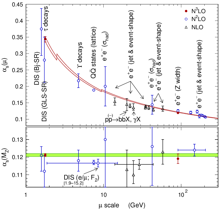
The theoretically most robust precision determination of $\alpha_{\scriptscriptstyle S}$ stems from the global fit to electroweak data at the $Z$ -mass scale. As for $\alpha_{\scriptscriptstyle S}(m_{\tau}^{2})$ , this determination benefits from the computation of the ${\rm N}^{3}{\rm LO}$ coefficient $K_{4}$ occurring in the radiator functions that predict the vector and axial-vector hadronic widths of the $Z$ (and also in the prediction of the total $W$ width). We use the newly developed Gfitter package [67] for the fit, and obtain

\displaystyle\alpha_{\scriptscriptstyle S}^{(Z)}(M_{Z}^{2})

\displaystyle=

\displaystyle 0.1191\pm 0.0027\pm 0.0001\>.

(35)

The value and first error represents the fit result, and the second error is due to the truncation of the perturbative series. It is estimated similarly to the $\tau$ case by adding a fifth-order term proportional to $K_{5}$ , estimated by $K_{4}(K_{4}/K_{3})$ , to the massless part, and a fourth-order term (estimated accordingly), containing large logarithms $\ln(\overline{m}_{t}/M_{Z})$ , to the massive part. We also vary the renormalisation scale of the massless contribution within the interval $\xi=1\pm 0.63$ , assuming the fifth order coefficient to be known. The result (35) agrees with the finding of Ref. [6].
The $\tau$ -based result (34) appears now twice more accurate than the determination from the $Z$ width. Yet the errors are very different in nature with a $\tau$ value dominated by theoretical uncertainties, whereas the determination at the $Z$ resonance, benefiting from the much larger energy scale and the correspondingly small uncertainties from the truncated perturbative expansion, is limited by the experimental precision of the electroweak observables. The consistency between the two results, $\alpha_{\scriptscriptstyle S}^{(\tau)}(M_{Z}^{2})-\alpha_{\scriptscriptstyle S}^{(Z)}(M_{Z}^{2})=0.0021\pm 0.0029$ , provides the most powerful present test of the evolution of the strong interaction coupling as it is predicted by the nonabelian nature of QCD over a range of $s$ spanning more than three orders of magnitude. The $\alpha_{\scriptscriptstyle S}^{(\tau)}(M_{Z}^{2})$ determination agrees with the average of the three currently most precise full NN(N)LO measurements (deep inelastic scattering [68, 60], ALEPH event shapes between 91 and 206 GeV [61], and global electroweak fit at $M_{Z}$ ), yielding an average of $0.1189\pm 0.0015$ ( $0.1204\pm 0.0009$ ) when not including (including) the $\tau$ result, which is justifiably assuming uncorrelated errors. The $\tau$ -based result differs at the $2.5\sigma$ level from the value $0.1170\pm 0.0012$ found in lattice QCD calculations with input from the mass splitting of the $\mathchar 28935\relax$ resonances [69]. The average of all five values reduces the discrepancy to $2.1\sigma$ ( $\chi^{2}$ probability of 0.04).

5 Conclusions

We have revisited the determination of $\alpha_{\scriptscriptstyle S}(m_{\tau}^{2})$ from the ALEPH $\tau$ spectral functions using recently available results. On the experimental side, new BABAR measurements of the $e^{+}e^{-}$ annihilation cross section into $K\kern 1.99997pt\overline{\kern-1.99997ptK}{}\pi$ using the radiative return method now permit, through CVC, a much more accurate determination of the vector/axial-vector fractions in the corresponding $\tau$ decays. Also, better results are available on $\tau$ decays into strange final states from BABAR and Belle. On the theory side, the first unknown term in the perturbative expansion of the Adler function, the fourth-order term $K_{4}$ , was recently calculated, opening the possibility to further push the accuracy of the theoretical analysis of the hadronic $\tau$ decay rate.
Motivated by these improvements we have reexamined the theoretical framework of the analysis. In particular the convergence properties of the perturbative expansions for the $\tau$ and $Z$ hadronic widths have been studied, and the ambiguity between the fixed-order (FOPT) and contour-improved (CIPT) approaches for summing up the series has been discussed. The study confirms our earlier findings (at third order) that CIPT is the more reliable treatment. Furthermore we have identified specific consistency problems of FOPT, which do not exist in CIPT. Possible violations of quark-hadron duality at the $\tau$ mass scale have been considered using specific models, and their effect has been found to be well within our quoted overall theoretical uncertainty (however, due to the coarseness of the models, we do not introduce additional theoretical errors).
We perform a combined fit of the $\tau$ hadronic width and hadronic spectral moments resulting in the value $\alpha_{\scriptscriptstyle S}(m_{\tau}^{2})=0.344\pm 0.005_{\rm exp}\pm 0.007_{\rm theo}$ , consistent with the previous value obtained for three known orders, and with a 20% reduced theoretical uncertainty. This somewhat moderate improvement is the result of the relatively large value $K_{4}\sim 49$ , suggesting a slowly converging perturbative series and giving rise to relatively large truncation uncertainties. Nevertheless, the result confirms the excellent accuracy that can be obtained from the analysis of $\tau$ decays, albeit indicating that this method may approach its ultimate accuracy.
The evolved $\tau$ result at the $M_{Z}$ scale, $\alpha_{\scriptscriptstyle S}(M_{Z}^{2})=0.1212\pm 0.0005_{\rm exp}\pm 0.0008_{\rm theo}\pm 0.0005_{\rm evol}$ , is the most accurate determination available. It agrees with the corresponding value directly obtained from $Z$ decays, which we have reevaluated. Both determinations are so far the only results obtained at ${\rm N}^{3}{\rm LO}$ order. They confirm the running of $\alpha_{\scriptscriptstyle S}$ between 1.8 and 91 $\mathrm{\,Ge\kern-1.00006ptV}$ as predicted by QCD with an unprecedented precision of 2.4%.

We are indebted to Martin Göbel and the Gfitter group for implementing the new ${\rm N}^{3}{\rm LO}$ term into the global electroweak fit, and AH acknowledges the fruitful collaboration. We thank Oscar Catà, Maarten Golterman and Santi Peris for letting us preview their analysis on duality violation in hadronic $\tau$ decays (which arrived after finalising this paper), and for helpful discussions. Many thanks to Matthias Jamin for pointing out a mistake in the total nonperturbative contributions previously quoted in Table 5 (corrected in the present version). This work was supported in part by the EU Contract No. MRTN-CT-2006-035482, “FLAVIAnet”.

References

[1] M. Davier, A. Höcker and Z. Zhang, Rev. Mod. Phys. 78, 1043 (2006) [hep-ph/0507078].
[2] S. Narison and A. Pich, Phys. Lett. B 211, 183 (1988).
[3] E. Braaten, Phys. Rev. D 39, 1458 (1989).
[4] E. Braaten, S. Narison and A. Pich, Nucl. Phys. B 373, 581 (1992).
[5] F. Le Diberder and A. Pich, Phys. Lett. B 289, 165 (1992).
[6] P. Baikov, K.G. Chetyrkin and J.H. Kühn, SFB-CPP-08-04, TTP08-01, arXiv:0801.1821 (2008).
[7] BABAR Collaboration (B. Aubert et al.), SLAC-PUB-12968, BABAR-PUB-07-052, arXiv:0710.4451 (2007).
[8] W. Marciano and A. Sirlin, Phys. Rev. Lett. 61, 1815 (1988).
[9] M. Davier, S. Eidelman, A. Höcker and Z. Zhang, Eur. Phys. J. C 27, 497 (2003) [hep-ph/0208177].
[10] Particle Data Group (W.M. Yao et al.), J. Phys. G 33, 1 (2006) and 2007 partial update for the 2008 edition.
[11] CKMfitter Group (J. Charles et al.), Eur. Phys. J. C 41, 1 (2005) [hep-ph/0406184]; updates at http://ckmfitter.in2p3.fr.
[12] ALEPH Collaboration (R. Barate, et al.), Eur. Phys. J. C 11, 599 (1999) [hep-ex/9903015].
[13] F. Mané et al. (DM1 Collaboration), Phys. Lett. B 112, 178 (1982).
[14] D. Bisello et al. (DM2 Collaboration), Z. Phys. C 52, 227 (1991).
[15] CLEO Collaboration (D. Asner, et al.), Phys. Rev. D 61, 012002 (2000) [hep-ex/9902022].
[16] CLEO Collaboration (T.E. Coan, et al.), Phys. Rev. Lett. 92, 232001 (2004) [hep-ex/0401005].
[17] J.J. Gomez-Cadenas, M.C. Gonzalez-Garcia and A. Pich, Phys. Rev. D 42, 3093 (1990).
[18] P. Roig, AIP Conf. Proc. 964, 40-46 (2007) [arXiv:0709.3734].
[19] M. Finkemeier and E. Mirkes, Z. Phys. C 69, 243 (1996) [hep-ph/9503474].
[20] BABAR Collaboration (B. Aubert et al.), Phys. Rev. Lett. 100, 011801 (2008) [arXiv:0707.2981].
[21] BABAR Collaboration (B. Aubert et al.), Phys. Rev. D-RC 76, 051104 (2007).
[22] Belle Collaboration (D. Epifanov et al.), Phys. Lett. B 654, 65 (2007) [arXiv:0706.2231].
[23] ALEPH Collaboration (D. Buskulic, et al.), Phys. Lett. B 307, 209 (1993).
[24] CLEO Collaboration (T. Coan, et al.), Phys. Lett. B 356, 580 (1995).
[25] OPAL Collaboration (K. Ackerstaff, et al.), Eur. Phys. J. C 7, 571 (1999) [hep-ex/9808019].
[26] F. Le Diberder and A. Pich, Phys. Lett. B 286, 147 (1992).
[27] A.A. Pivovarov, Sov. J. Nucl. Phys. 54, 676 (1991); Z. Phys. C 53, 461 (1992).
[28] G. Grunberg, Phys. Lett. B 95, 70 (1980), Erratum-ibid. B 110, 501 (1982).
[29] G. Grunberg, Phys. Rev. D 29, 2315 (1984).
[30] A. Dhar, Phys. Lett. B 128, 407 (1983).
[31] A. Dhar and V. Gupta, Phys. Rev. D 29, 2822 (1983).
[32] P.M. Stevenson, Phys. Rev. D 23, 2916 (1981).
[33] P. Ball, M. Beneke and V.M. Braun, Nucl. Phys. B 452, 563 (1995) [hep-ph/9502300].
[34] G. Altarelli, P. Nason and G. Ridolfi, Z. Phys. C 68, 257 (1995) [hep-ph/9501240].
[35] M. Neubert, Nucl. Phys. B 463, 511 (1996) [hep-ph/9509432].
[36] ALEPH Collaboration (R. Barate, et al.), Z. Phys. C 76, 15 (1997).
[37] ALEPH Collaboration (R. Barate, et al.), Eur. Phys. J. C 4, 409 (1998).
[38] M.A. Shifman, A.L. Vainshtein and V.I. Zakharov, Nucl. Phys. B 147, 385, 448, 519 (1979).
[39] E. Poggio, H. Quinn and S. Weinberg, Phys. Rev. D 13, 1958 (1976).
[40] E. Braaten, Phys. Rev. Lett. 60, 1606 (1988).
[41] M.A. Shifman, Quark-hadron duality, Boris Ioffe Festschrift At the Frontier of Particle Physics, Handbook of QCD, M.A. Shifman (ed.), World Scientific, Singapore, 2001, hep-ph/0009131.
[42] O. Cata, M. Golterman and S. Peris, JHEP 0508, 076 (2005) [hep-ph/0506004].
[43] E. Braaten and C.S. Li, Phys. Rev. D 42, 3888 (1990).
[44] O. Cata, M. Golterman and S. Peris, arXiv:0803.0246 (2008).
[45] S. Adler, Phys. Rev. D 10, 3714 (1974).
[46] L.R. Surguladze and M.A. Samuel, Phys. Rev. Lett. 66, 560 (1991), Erratum-ibid. 66, 2416 (1991).
[47] S.G. Gorishnii, K.L. Kataev and S.A. Larin, Phys. Lett. B 259, 144 (1991).
[48] K.G. Chetyrkin, A.L. Kataev and F.V. Tkachov, Phys. Lett. 85, 277 (1979).
[49] M. Dine and J.R. Sapirstein, Phys. Rev. Lett. 43, 668 (1979).
[50] W. Celmaster and R.J. Gonsalves, Phys. Rev. Lett. 44, 560 (1980).
[51] S.A. Larin, T. van Ritbergen and J.A.M. Vermaseren, Phys. Lett. B 400, 379 (1997) [hep-ph/9701390]; Phys. Lett. B 404, 153 (1997) [hep-ph/9702435].
[52] A.L. Kataev and V.V. Starshenko, Mod. Phys. Lett. A 10, 235 (1995) [hep-ph/9502348].
[53] C.J. Maxwell and D.G. Tonge, Nucl. Phys. B 481, 681 (1996) [hep-ph/9606392]; Nucl. Phys. B 535, 19 (1998) [hep-ph/9705314].
[54] P.A. Raczka, Phys. Rev. D 57, 6862 (1998) [hep-ph/9707366].
[55] J.G. Körner, F. Krajewski and A.A. Pivovarov, Phys. Rev. D 63, 036001 (2001) [hep-ph/0002166].
[56] D.J. Broadhurst, Z. Phys. C 58, 339 (1993).
[57] M. Beneke and V.M. Braun, Phys. Lett. B 348, 513 (1999) [hep-ph/9411229].
[58] D.J. Broadhurst and S.C. Generalis, Phys. Lett. 165, 175 (1985).
[59] ALEPH Collaboration (S. Schael, et al.), Phys. Rept. 421, 191 (2005) [hep-ex/0506072].
[60] S. Bethke, Prog. Part. Nucl. Phys. 58, 351 (2007) [hep-ex/0606035].
[61] G. Dissertori et al., JHEP 0802, 040 (2008) [arXiv:0712.0327].
[62] K.G. Chetyrkin, B.A. Kniehl and M. Steinhauser, Phys. Rev. Lett. 79, 2184 (1997) [hep-ph/9706430]; Nucl. Phys. B 510, 61 (1998) [hep-ph/9708255].
[63] J. Schieck et al., Eur. Phys. J. C48, 3 (2006), Erratum-ibid. 50, 769 (2007) [arXiv:0707.0392].
[64] W. Bernreuther and W. Wetzel, Nucl. Phys. B 197, 228 (1982); Erratum ibid. B 513, 758 (1998).
[65] W. Wetzel, Nucl. Phys. B 196, 259 (1982).
[66] G. Rodrigo, A. Pich and A. Santamaria, Phys. Lett. B 424, 367 (1998) [hep-ph/9707474].
[67] Gfitter Group (M. Göbel et al.), Programme library for electroweak fits and beyond (publication in preparation); more information at: https://twiki.cern.ch/twiki/bin/view/Gfitter/WebHome.
[68] J. Santiago and F.J. Ynduráin, Nucl. Phys. B 611, 447 (2001).
[69] Q. Mason et al., Phys. Rev. Lett. 95, 052002 (2005).

The Determination of 𝜶𝑺\alpha_{\scriptscriptstyle S} from 𝝉\tau Decays Revisited