Tilted anisotropic Dirac cones in quinoid-type graphene and (BEDT-TTF)2I3
Abstract
We investigate a generalized two-dimensional Weyl Hamiltonian, which may describe the low-energy properties of mechanically deformed graphene and of the organic compound (BEDT-TTF)2I3 under pressure. The associated dispersion has generically the form of tilted anisotropic Dirac cones. The tilt arises due to next-nearest-neighbor hopping when the Dirac points, where the valence band touches the conduction band, do not coincide with crystallographic high-symmetry points within the first Brillouin zone. Within a semiclassical treatment, we describe the formation of Landau levels in a strong magnetic field, the relativistic form of which is reminiscent to that of graphene, with a renormalized Fermi velocity due to the tilt of the Dirac cones. These relativistic Landau levels, experimentally accessible via spectroscopy or even a quantum Hall effect measurement, may be used as a direct experimental verification of Dirac cones in (BEDT-TTF)2I3.
pacs
73.61.Wp, 73.61Ph, 73.43.-fI Introduction
The discovery of a particular quantum Hall effect in graphene[1, 2] has shown that the low-energy electronic properties in this two-dimensional (2D) carbon crystal are described not in terms of a Schrödinger-type wave equation but by a relativistic Dirac equation.[3] Due to a -band, which shrinks at half-filling to two inequivalent points at the corners of the first Brillouin zone (BZ), the electronic energy dispersion is almost linear resulting in Dirac cones. This is reminiscent of the case of massless relativistic particles, where the speed of light is replaced by a Fermi velocity , which is roughly 300 times smaller than .
Another material where Dirac cones are expected to occur is the organic 2D compound (BEDT-TTF)2I3 under pressure.[4, 5, 6] The relativistic behavior of the carriers may be at the origin[4] of an experimentally observed dependence of the carrier density.[7, 8] Whereas in graphene, the Dirac cones at the corners of the first BZ are isotropic, they are situated within the first BZ in (BEDT-TTF)2I3, strongly anisotropic, and tilted in the wave-vector energy space ().[4, 5] The electronic properties are described by a generalized Weyl Hamiltonian with terms linear in the 2D wave vector . However, in contrast to graphene, there is yet no direct experimental evidence for the presence of Dirac cones in (BEDT-TTF)2I3 or whether the system is simply a narrow-gap semiconductor.
In the present paper, we study the structure of the generalized Weyl Hamiltonian, which yields energy dispersions in form of tilted anisotropic Dirac cones. In the presence of a strong magnetic field, the dispersion is quantized in relativistic Landau levels (LLs), with the characteristic behavior known from graphene. The tilt and the anisotropy of the Dirac cones give rise to a renormalization of the effective Fermi velocity and therefore of the typical LL spacing.
One example of a 2D system described by such generalized Weyl equation may be the above-mentioned organic material (BEDT-TTF)2I3. We show, within an effective tight-binding model on an anisotropic triangular lattice with two atoms per unit cell,[9] that the tilting of the Dirac cones is due to next-nearest-neighbor (nnn) hopping, which may be in (BEDT-TTF)2I3 on the same order of magnitude as nearest-neighbor (nn) hopping.[10, 11] A necessary condition for nnn hopping to cause a tilt of the Dirac cones is that they are situated at points in the first BZ different from those of high crystallographic symmetry, such as its corners. Furthermore, we show that it may equally apply to graphene when the Dirac points, and move away from the high-symmetry points and at the corners of the first BZ. In this case the wave-vector expansion of the nnn term yields a linear contribution, whereas it is quadratic when the Dirac points coincide with the BZ corners and . Such motion of the Dirac points may indeed be induced by a quinoid-type lattice distortion[12] of the graphene sheet. However, we show that the tilt of the Dirac cones is much less pronounced than in (BEDT-TTF)2I3. Alternatively, this motion of Dirac points may be studied in cold atoms in an optical lattice where one may deform the honeycomb lattice and fine-tune the nn and nnn hopping parameters with the help of the laser intensities, wavelengths, and relative orientation.[13]
The paper is organized as follows. We start with a theoretical discussion of the generalized Weyl Hamiltonian in Sec. II. Sec. III is devoted to the LL formation in a strong magnetic field, for the case of tilted Dirac cones. Possible experimental realizations in distorted graphene and (BEDT-TTF)2I3 are discussed in Sec. IV, which we conclude with an analysis of a possible quantum Hall effect in (BEDT-TTF)2I3.
II Generalized Weyl Hamiltonian
We consider a model of two-spinor fermions restricted to a 2D space. Whereas the two-spinor form is in general dictated by relativistic invariance in two space dimensions, it naturally arises in the condensed matter situation of a lattice with two inequivalent sites. The most general Hamiltonian linear in the 2D wave vector , is given by the “generalized Weyl Hamiltonian”,
| (1) |
in terms of the velocities , and the Pauli matrices . Here and in the following parts, we choose a unit system with . Both 2D space components of the velocities, and , are in themselves vectors in the 4D spin space [the space of SU(2) matrices] spanned by the Pauli matrices. The usual 2D Weyl Hamiltonian, which describes for instance low-energy massless electrons in graphene,[3] is included in (1) if one considers , , and , in terms of the Fermi velocity .
Although, at first sight, the Weyl Hamiltonian is described by eight different parameters, given by the four two-component velocities , it is indeed overspecified. In order to illustrate this point, we rewrite the Hamiltonian (1) in a different manner,
| (2) |
One may get rid of two parameters () by choosing the 3-quantization axis in the SU(2) space perpendicular to the vectors and .
This point is indeed remarkable and needs to be discussed in the light of graphene physics. In this case, a constant term breaks the inversion symmetry of the honeycomb lattice, e.g. due to a different on-site energy of the two triangular sublattices. Usually, this gives rise to a mass term and breaks the particle-hole symmetry. In the generalized Weyl Hamiltonian, this is not the case because the term is linear in the wave vector and therefore does not affect the zero-energy state at .
One may furthermore reduce the number of relevant model parameters by a simple rotation of the 2D frame of reference, accompanied by a unitary transformation in the SU(2) space, which leaves the 3-quantization axis invariant. One, thus, obtains the “minimal” Weyl Hamiltonian
| (3) |
in terms of the four effective velocities , and . A detailed discussion of the involved transformations and a derivation of the exact expressions for the effective velocities may be found in the Appendix A.
The diagonalization of the minimal Weyl Hamiltonian yields the energy dispersions
| (4) |
where plays the role of the band index.

For and , one obtains the isotropic model, which applies e.g. to the low-energy electronic properties in graphene: the Fermi velocities are the same in the - and -direction. The rotational symmetry is broken if (anisotropic model). Such case may be obtained e.g. if the graphene sheet is constrained by a uniaxial pressure, as is discussed in Sec. IV A. For , the Dirac cones are tilted away from the -axis, as is shown in Fig. 1.
Notice that not all values of the tilt parameter are indeed physical. In order to be able to associate to a positive and to a negative energy state, one obtains the condition
| (5) |
Unless this condition is satisfied, the iso-energetic lines are no longer ellipses but hyperbolas. Notice that, here, we aim to use the generalized Weyl Hamiltonian (1) and its resulting energy dispersion (4) to describe the electronic properties of particular 2D materials. Although it may be interesting to speculate about the resulting properties of a model that violates the condition (5), we are not aware of any physical example which might correspond to such a case.
In a 2D lattice system with valley degeneracy, a generalized Weyl Hamiltonian may describe the low-energy excitations in different valleys separately. In the remainder of this paper, we will in general only consider a single valley (and explicitly mention the inclusion of the twofold valley degeneracy when needed). Note also that we do not consider the true electron spin and do not include the corresponding twofold spin degeneracy.
In order to discuss the symmetry properties of the generalized Weyl Hamiltonian (3), it is convenient to introduce the unitary and Hermitian chirality operator
| (6) |
which commutes naturally with the Hamiltonian. The associated eigenvalues are and coincide with the band indices . As exemplified in Sec. IV, this is generally not the case in a physical condensed-matter situation – the Weyl Hamiltonian corresponds to the effective model at Dirac points, where the conduction band touches the valence band; these Dirac points occur in pairs, at inequivalent points in the first BZ, which yields a twofold valley degeneracy. In this case, the effective model is rather given by , where denotes the two valleys, and the relation between band index, chirality, and valley index is given by
| (7) |
In the present discussion, we may however identify the band index with the chirality, for simplicity.
The eigenstates of the chirality operator are
| (8) |
where . These eigenstates are also the natural eigenstates for the generalized Weyl Hamiltonian.
III Tilted Dirac Cones in a Magnetic Field
We use the Peierls substitution to obtain the generalized Weyl Hamiltonian in a magnetic field
| (9) |
where is the vector potential that generates the (uniform) magnetic field perpendicular to the 2D plane. With the help of the ladder operators
| (10) |
in terms of the magnetic length , one obtains the Hamiltonian
| (11) |
where we have defined
in terms of the effective tilt parameter
| (12) |
Instead of the full solution of the Hamiltonian (11), we consider the effect of the magnetic field in a semiclassical treatment. The Onsager relation[14] states that the surface enclosed by a trajectory of constant energy in reciprocal space is quantized as
where is an integer denoting the energy level which coincides with the Landau level in the full quantum treatment. The additional contribution is related to a Berry phase acquired by an electron during its cyclotron orbit. Usually, one has except if there is an extra Berry phase of , which in our case yields , as in the case of graphene with no tilt.[15] If one considers a density of states which scales as , the energy levels thus scale as
| (13) |
in the large- limit. In usual (non-relativistic) 2D electron systems, one finds a constant density of states, i.e. , and . The scaling of the conventional Landau levels is therefore . In the relativistic case of electrons in graphene, the density of states vanishes linearly at the Dirac points, and one therefore obtains because and . The relation (13) has been generalized to the case of a spatially anisotropic density of states by Dietl et al. [16]
From the scaling argument (13) in the large- limit, one may notice that the -field scaling of the levels must be the same as the scaling. Furthermore, one sees from the quantum Hamiltonian (11) that the energy must scale as . Therefore, the energy levels must obey, in the large- limit, the equation
| (14) |
as in the case of the Weyl equation for massless charged particles, such as in graphene, apart from a renormalization of the Fermi velocity.
The renormalization of the Fermi velocity may be obtained from the calculation of the density of states. The total number of states below a given energy within the positive energy cone is given by
where we have defined , and the renormalized Fermi velocity is written in integral form,
| (15) |
in terms of the effective tilt parameter (12). One notices from Eq. (15) that if the condition (5), , is not satisfied, the expression under the integral diverges because the denominator may become zero. This result is not suprising because the Onsager quantization relation, which yields the energy levels (14) is only valid for closed orbits, given e.g. by the elliptic isoenergetic lines. As already mentioned, the orbits for are open hyperbolas, and the expression (14) is no longer valid.
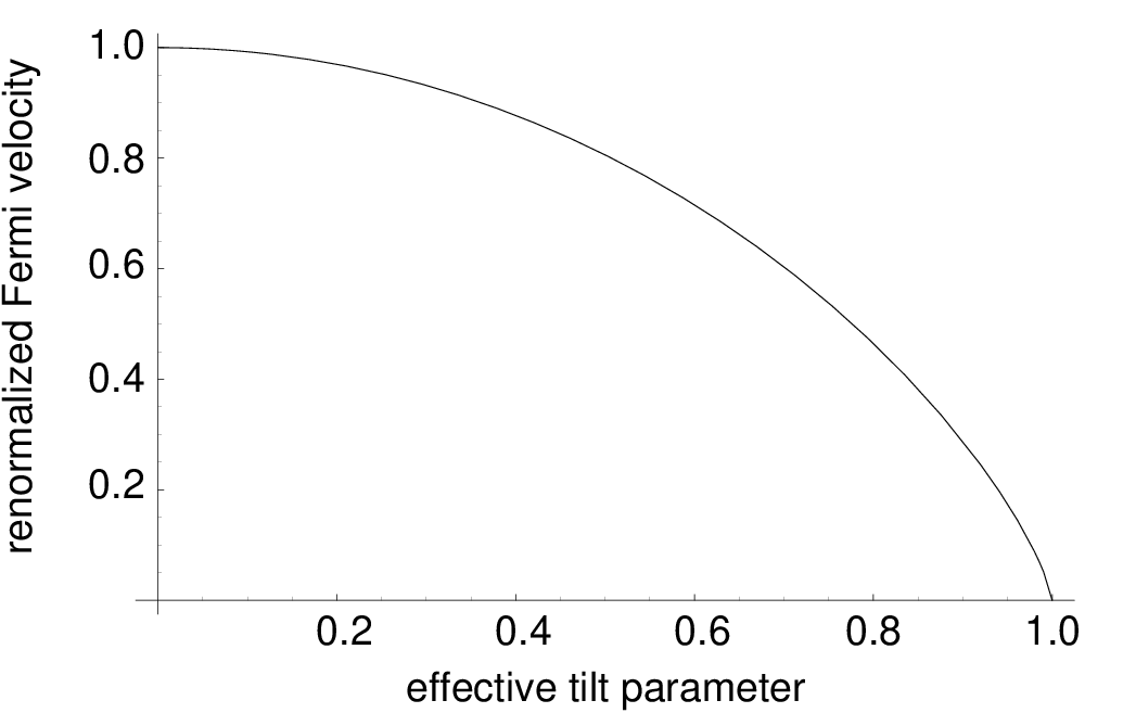
The density of states is obtained by differentiation of the number of states,
| (16) |
which is the concise expression for both the positive and negative parts of the tilted Dirac cones.
The behavior of Eq. (14) is, strictly speaking, valid only in the large- limit. However, usually it yields extremely good estimates for the levels down to values as small as . Special care is needed for the discussion of the level, which requires a quantum treatment of the Hamiltonian (11). In the following, we discuss the fate of the zero-energy Landau level.
The behavior of this level may be understood with the help of the quantum treatment of the Hamiltonian for . In this case, the expression (14) is exact with , which is also the -limit of the expression (15). There exists thus a zero-energy level for , which has the same degeneracy, as all other levels , in terms of the number of flux quanta threading the total surface .
For non-zero values of , the Hamiltonian (11) may not be diagonalized by a simple canonical transformation. However, the Hamiltonian (11) is transformed as under space inversion, , as shown in the Appendix B. This implies that the energy spectrum is symmetric around zero energy (see Appendix B). Therefore, starting from and adiabatically turning on , there are only two possibilities for the evolution of the zero-energy level: (i) either it remains at zero energy or (ii) it splits into (at least) two sublevels and , which are symmetric around zero energy. However, splitting of the zero-energy level into sublevels can be excluded on account of the degeneracy of this level. Indeed, when , the exact degeneracy of the zero energy () Landau level is given by (remember that we only consider a single valley here). When , it can, therefore, not split since this would indeed lead to an unphysical doubling of the number of quantum states because each level, and , would have to be times degenerate. Therefore, for all magnetic field strength, there exist a zero-energy Landau level. The explicit expressions for the zero-energy wave functions may be found in the Appendix C. Notice, that this is consistent with the semiclassical spectrum with .
In the above treatment, we only considered a single valley. We note however that the magnetic field might introduce a coupling between the two valleys. In such a case, we do not exclude a parity anomaly which consists of a different behavior of the level at the two inequivalent Dirac points at non-zero wave vectors in a lattice model. In this case, space inversion would involve the low-energy Hamiltonians at both Dirac points, and the spectrum is only symmetric around zero energy if one accounts for both valleys. The parity anomaly is, however, expected to play no physical role in the continuum limit with , where is the lattice spacing.
In conclusion, we have obtained the semiclassical spectrum of Landau levels [see Eqs (14)-(12], valid when ) and checked that the zero energy level () indeed exists in a full quantum treatment. Based on this two calculations, we expect the semiclassical spectrum to be a very good approximation to the true quantum spectrum of Landau levels, for all . This is one of the main result of the present paper.
IV Physical Examples of Tilted Dirac Cones
After this rather technical discussion of the generalized Weyl Hamiltonian and tilted Dirac cones, we discuss, here, two physical systems which may display these properties. We find that whereas the tilt of the Dirac cones is well pronounced and thus strongly affects the Landau level quantization in (BEDT-TTF)2I3, it is much more difficult to induce a tilt in graphene via a lattice deformation. However, a quinoid-type lattice deformation is also discussed for pedagogical reasons because the general physical origin of tilted Dirac cones becomes transparent.
IV.1 Quinoid-type graphene under uniaxial strain

As a first example, we consider a graphene sheet which is deformed in one of its principle symmetry axes. This particular deformation results in a quinoid variety of the honeycomb lattice.[17] We treat its electronic properties within the tight-binding approximation. Starting from the graphene honeycomb lattice, with equal bond length nm and equal nn hopping energy eV, the bond length and hopping energy are modified in the deformation axis (see Fig. 3),
and kept unchanged otherwise. We call the relative strain. Here, we consider a moderate deformation, , such that one may linearize the hopping energy around its nondeformed value , and eV/.[17, 18] This value agrees with an evaluation based on Harrison’s law[19] according to which , where is a numerical prefactor of order one. Derivation with respect to yields
| (17) |
For simplicity and as a first approximation, one may keep the bond angles fixed at . The underlying Bravais lattice is no longer triangular but oblique with the basis vectors
and the reciprocal lattice is spanned by the vectors
Furthermore, we take into account nnn hopping, with a characteristic energy of[20] in the undeformed horizontal axes. The deformation yields, in the same manner as for the nn hopping energies, different hopping energies for the other directions (see Fig. 3),
The tight-binding model may be described by the Hamiltonian
| (18) |
in reciprocal space, where and are the Fourier components of the annihilation (creation) operators on the A and B sublattices, respectively. The Hamiltonian matrix
is given in terms of the elements
| (19) | |||||
and
| (20) | |||||
The energy dispersion is obtained from the eigenvalues of ,
| (21) |
and is plotted in Fig. 4 for a deformation of . The two bands, and , touch each other at the Dirac points , which are obtained from the condition ,[16]
| (22) |
where denotes the two inequivalent Dirac points and , respectively. In the absence of any distortion, the Dirac points and coincide with the crystallographic points and , respectively, at the corners of the first BZ. The distortion makes both pairs of points move in the same direction due to the negative value of . However, unless the parameters are fine-tuned, this motion is different, and the two pairs of points no longer coincide.[21]

The low-energy properties of electrons in a quinoid-type distorted graphene sheet are described by the linearized model around the Dirac points, which is exactly of the form (3) of the Weyl Hamiltonian,
| (23) |
with the effective velocities
| (24) | |||||
where we have defined . The corresponding energy dispersion is independent of , which is at the origin of the twofold valley degeneracy. In order to obtain the concise form of Eq. (23), we have chosen the spinor representation at the Dirac point and for , i.e. interchanged the sublattice components at . As mentioned in Sed. II, the relation between the band index , chirality , and valley index is given by Eq. (7), , due to the global sign in the Hamiltonian (23). The constant term has been absorbed in a renormalization of the chemical potential, the position of which is determined by the electronic half-filling of the graphene sheet.
One notices from the Eqs. (24) that the quinoid-type distortion yields an anisotropy in the Fermi velocities, , and that the Dirac cones are tilted due to . The isotropic graphene model is retrieved at – one has then eVÅ and because , , and , in the undeformed case. Without deformation, nnn hopping therefore does not affect the energy dispersion at linear order, but only at second order. This is due to the fact that the Dirac points are then situated at the high-symmetry crystallographic points and . Indeed, this yields a parabolic correction, which breaks the original electron-hole symmetry.[3, 22]
To summarize, in order to obtain tilted Dirac cones in graphene, two ingredients are required: (i) nnn hopping, which generates the diagonal components in the Hamiltonian (18); and (ii) for a linear contribution arising from this term, the Dirac points and need to be shifted away from the high-symmetry points and . This shift may be obtained by constraining the graphene sheet into such a quinoid type.
In the presence of a magnetic field, the LL spacing is affected by the deformation because the Fermi velocity is renormalized according to Eq. (15),
| (25) |
for small values of the effective tilt parameter . It may be evaluated from the model parameters,
| (26) | |||||
In order to estimate , we use the “atomic orbitals overlap law” familiar in the context of the extended Hückel model,[23]
where is the nn distance, is the nnn distance, and Å is a caracteristic distance related to the overlap of atomic orbitals. In the undeformed graphene , whereas in the quinoid type graphene and . This gives and . Therefore, the effective tilt parameter is given by
As the correction to the Fermi velocity appears as [see Eq. (25)], this effect remains extremely small, and the tilt affects the LL spacing in a negligible manner.
The main contribution to the renormalized Fermi velocity therefore arises not from the tilt of the Dirac cones (effect of order ), but from the anisotropy in the Fermi velocities (effect of order ), and one finds
| (27) |
which may yield an experimentally observable effect in the percent range for a strain of .
¿From an experimental point of view, such quinoid-type deformation may be realized if one uses a piezoelectric substrate, on which the graphene sheet is posed, instead of the most commonly used SiO2. Another possibility would be to use a mechanical deformation of the underlying substrate. Such bending has been exploited e.g. to investigate carbon nanotubes under strain.[24] More recently, graphene on polydimethylsiloxane (PDMS) has been put under uniaxial strain by bending of the PDMS.[25] The elastic regime in graphene requires that the strain is smaller than and the rupture occurs around . Therefore an upper bound for is certainly .
IV.2 Organic 2D compounds
Another example of a 2D metal, where tilted Dirac cones may occur, is the layered organic compound (BEDT-TTF)2I3 under (uniaxial) pressure.[4, 5, 6] Each layer may be described by an oblique lattice with four sites per unit cell, and the electronic filling is . In the vicinity of the Fermi energy, only two out of the four bands are relevant for the low-energy electronic properties. It has indeed been shown that the band structure may be modeled with great precision within a tight-binding model on a half-filled anisotropic triangular lattice with nn and nnn hopping, where each site corresponds to a dimer.[9] This is a natural assumption for - and -(BEDT-TTF)2I3, where there exists one hopping energy which is largely enhanced with respect to the others. In contrast to these compounds, the assumption may seem hasardous at first sight in the case of (BEDT-TTF)2I3, where there is no such clearly enhanced hopping energy, such that the dimerization is expected to be rather weak. Furthermore, these organic materials exhibit strong electronic correlations, and a tight-binding calculation for quasi-free electrons sweeps a lot of interesting physics under the carpet. However, the high-pressure limit corresponds to a regime where the electrons are less strongly correlated and where interaction effects may be taken into account via renormalized effective hopping parameters.[5]
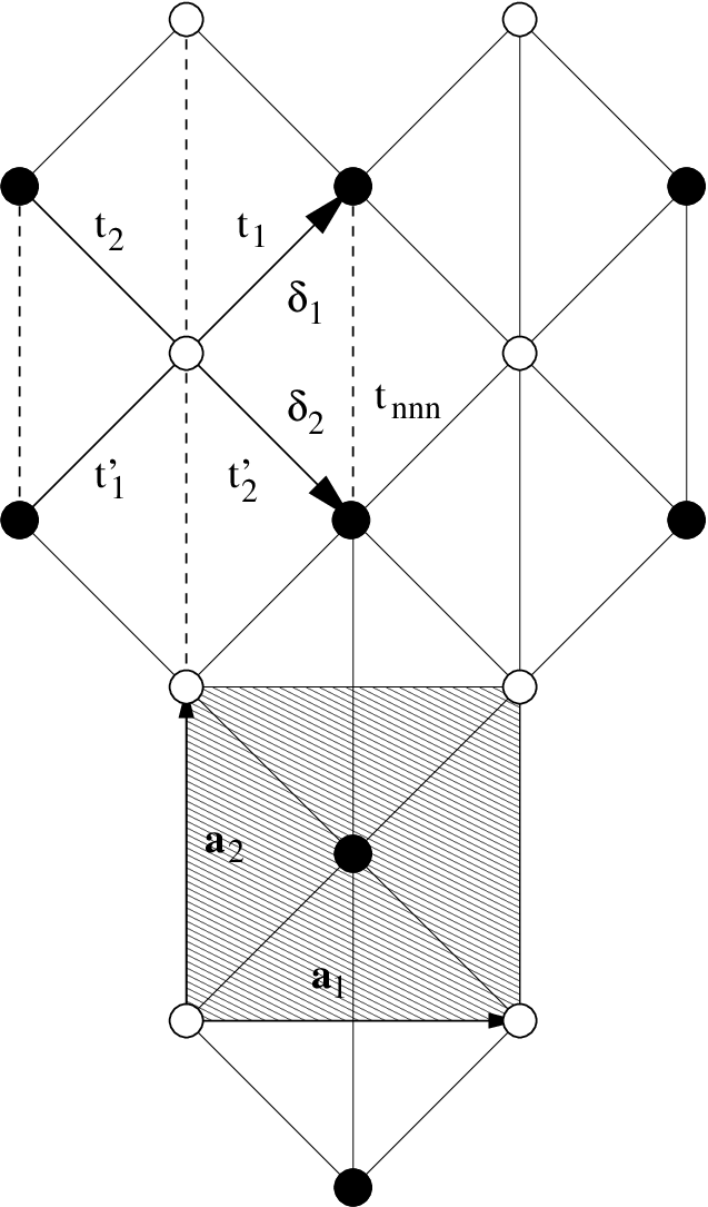
The tight-binding model on the anisotropic triangular lattice is depicted in Fig. 5. The nn are situated at the vectors and , with
which connect sites on the different sublattices, and and the vectors
span the underlying Bravais lattice, which is chosen to be a square lattice, for simplicity. Notice that the lattice may also be viewed as an anisotropic 2D NaCl lattice (two inequivalent interpenetrating square lattices). The bond length is set to unity, . The nn hopping energies are and in the directions , and and in the directions , respectively. The nnn hopping energy is .
The effective tight-binding model may be written in the same manner (18) as for the case of quinoid-type graphene, with the matrix elements
and
The energy dispersion is obtained from Eq. (21), and the position of the Dirac points is calculated from
One may directly see that the r.h.s of both equations must be positive in order to have a pair of Dirac points ( and ) within the first BZ, .
An expansion around the Dirac points yields the generalized Weyl Hamiltonian (1),
in terms of the velocities
Here, we have used the same spinor representation as for quinoid-type graphene, i.e. we have interchanged the sublattice components when changing the valley. One notices that the Dirac cones are tilted only if the Dirac points are not situated at the border of the first BZ, . This corresponds to the high-symmetry crystallographic points in graphene, and nnn hopping affects the effective model again only at second order in the expansion around the Dirac points.
The experimental evidence for (tilted) Dirac cones in (BEDT-TTF)2I3 compounds under pressure is yet rather weak. Whereas at ambiant pressure, the material is an insulator due to charge ordering, temperature-dependent transport measurements under high hydrostatic pressure have revealed a dependence of the carrier density below K,[7, 8] as one would expect for relativistic electrons with a linear dispersion relation.[4, 3] It is, however, not clear whether the compound has, under these circumstances, a truely vanishing gap as for massless relativistic electrons or whether a tiny gap persists. Furthermore the dependence of the carrier density is accompanied by a temperature-dependent mobility, which results in an essentially constant conductivity over a large temperature range.[8]
A more direct evidence for the relevance of Dirac cones in (BEDT-TTF)2I3 would be a measurement of the characteristic properties of relativistic quantum Hall physics, as in the case of graphene.[1, 2, 3] The following final part of this paper is devoted to the discussion of possible quantum Hall physics in (BEDT-TTF)2I3.
Possible quantum Hall effect in (BEDT-TTF)2I3
Although it is a delicate issue to yield energy values for the hopping parameters and from the overlap integrals in (BEDT-TTF)2I3,[10, 11] we expect that the good agreement between band-structure calculations in the full model with four sites per unit cell and the anisotropic triangular lattice model[9] yields the correct orders of magnitude for the effective velocities (IV.2). Using the prescription proposed by Hotta[9] and the overlap integrals calculated by Mori et al.,[10] we may estimate meV, meV, meV, meV, and meV. These values yield a pair of Dirac points at and , with , in units of the inverse lattice constant, which is on the order of Å.[10, 11, 26] With the help of Eqs. (IV.2), one thus obtains the effective velocities eVÅ, eVÅ, eVÅ, eVÅ, , and eVÅ. One notices a variation by almost two orders of magnitude, and one may therefore expect rather large anisotropies.
The effective velocities in the minimal model are calculated with the help of Eqs. (32), and one finds a rotation angle of and the velocities eVÅ, eVÅ, eVÅ, and eVÅ. The average Fermi velocity is therefore eVÅ, which is roughly one order of magnitude smaller than that in graphene. The tilt parameter (12) is
and thus much larger than in the case of a quinoid-type deformation of a graphene sheet. The tilt therefore leads to a reduction of the average Fermi velocity, and one finds from Eq. (25) a renormalized velocity of
The renormalized Fermi velocity allows one to extract the typical energy scale for the Landau levels in (BEDT-TTF)2I3, and one finds from Eq. (14) , with a characteristic “cyclotron” frequency of
| (29) |
which is, due to the smaller Fermi velocity, roughly one order of magnitude smaller than that in graphene. However, this energy scale is comparable to the cyclotron frequency in GaAs heterostructures ( meV), which are most commonly used in the study of quantum Hall physics.[27] One may therefore expect that a relativistic quantum Hall effect[1, 2] could principally also occur in (BEDT-TTF)2I3 if disorder does not prevent LL formation.
Experimentally, thin (BEDT-TTF)2I3 films have already been synthesized.[28] Alternatively, one may hope that the exfoliation technique,[29] which has proven to be particularly successful in the fabrication of single-layer graphene sheets, also yields reasonably thin (BEDT-TTF)2I3 samples. However, (BEDT-TTF)2I3 crystals are generally of lower mechanical stability than carbon crystals, due to the relatively large lattice constants and the reduced binding energies.
Apart from a direct measurement of a quantum Hall effect in (BEDT-TTF)2I3 compounds, one may probe the system via transmission spectroscopy in a magnetic field. This would allow for a direct measurement of the cyclotron frequency and for a check of the relativistic character of electrons in (BEDT-TTF)2I3. Transmission spectroscopy has indeed been successfully applied to epitaxial[30] and exfoliated[31] graphene and yields a scaling of the transmission lines, as expected for the relativistic quantum Hall effect in graphene.
V Conclusions
In conclusion, we have investigated tilted Dirac cones in deformed graphene and the organic 2D material (BEDT-TTF)2I3. The low-energy electronic properties are described by a generalized Weyl Hamiltonian, which may in both physical systems be derived from a tight-binding model on a lattice with two inequivalent sites. Whereas the presence of pairs of Dirac points is due to nn hopping, which couples neighboring sites on inequivalent sublattices, the tilt of the Dirac cones arises from nnn hopping if the Dirac points are shifted away from the points of high crystallographic symmetry in the first Brillouin zone.
In the presence of a strong magnetic field, a semiclassical analysis yields the same structure of relativistic LLs as in non-deformed graphene, but with a renormalized effective Fermi velocity due to the tilt and the anisotropy of the Dirac cones. Whereas this effect is expected to be small in a quinoid-type deformation of the graphene, our estimates for the effective velocities for (BEDT-TTF)2I3 indicate that the tilt yields a significant reduction of the effective Fermi velocity, which determines the LL spacing. The largest spacing of the and LL transitions is on the order of meV, which is on the order of the (equidistant) LL spacing in GaAs heterostructures most commonly used in quantum Hall effect measurements. Such measurements in (BEDT-TTF)2I3, as well as LL spectroscopy, may be a possible experimental verification of the yet weakly corroborated presence of Dirac cones in (BEDT-TTF)2I3.
Acknowledgments
We acknowledge fruitful discussions with Hélène Bouchiat, Natasha Kirova, Claude Pasquier, Jean-Paul Pouget, and Yoshikazu Suzumura. This work is partially supported by the Agence Nationale de la Recherche under Grant No. ANR-06-NANO-019-03.
Appendix A Derivation of the minimal Weyl Hamiltonian
In order to reduce the number of effective parameters in the Weyl Hamiltonian (2), one rotates the 2D reference system in the physical space,
accompanied by a unitary transformation in the SU(2) space,
which leaves the -quantization axis invariant and describes a rotation in the -plane in the SU() spin space,
| (30) | |||||
| (31) |
If one chooses
and
one obtains the “minimal” Weyl Hamiltonian (3). In terms of the original velocities, the minimal set of effective parameters (the velocities , and ) reads
| (32) | |||||
Appendix B Transformation of the Weyl Hamiltonian under space inversion
The ingredients which intervene in the Peierls substitution (9), , are vectors, which transform as under space inversion. Because of this transformation property and because the generalized Weyl Hamiltonian (1) is linear in the momentum, we have
| (33) |
in space representation, where is given in Eq. (11). We now consider a solution of the Schrödinger equation,
of energy . Due to the property (33) under space inversion, one finds that
| (34) |
This means that is a solution of the Schrödinger equation with energy , and to each energy in the upper energy band there exists one at in the lower one. The resulting Landau level energy spectrum is, therefore, symmetric around zero energy.
Notice, however, that this argument is only valid for the generalized Weyl Hamiltonian if one neglects the underlying lattice model for which the Weyl Hamiltonian describes the low-energy properties. As mentioned in the text, Dirac points occur in pairs at non-zero wave vectors, and one thus obtains a twofold valley degeneracy . In this case, there is a relative minus sign between the two copies of the Weyl Hamiltonian . Space inversion, therefore, becomes an exact symmetry of the model and involves both valleys.
Appendix C Zero-energy Landau level for the case with tilt
In this appendix, we show that there exists a zero energy mode for the Hamiltonian (11). We may represent the ladder operators and as
which act on states described as functions of the real variable . The latter is not necessarily identical to the - or -variable in the plane, but should rather be viewed as an auxiliary variable that allows for a formal solution of the zero-energy problem.
The Hamiltonian (11), thus, reads
| (35) |
and we may search the solutions of the zero-energy eigenvalue equation, , with the ansatz
This yields the system of linear equations
which has a non-zero solution if we choose
| (36) |
and, thus,
Notice that we only obtain bound states, i.e. states that decay at large values of , for ( and real), which corresponds to the maximal-tilt condition (5).
References
- [1] K. S. Novoselov, A. K. Geim, S. V. Morosov, D. Jiang, M. I. Katsnelson, I. V. Grigorieva, S. V. Dubonos, and A. A. Firsov, Nature 438, 197 (2005).
- [2] Y. Zhang, Y.-W. Tan, H. L. Stormer, and P. Kim, Nature 438 201, (2005).
- [3] For a recent review, see A. H. Castro Neto, N. M. R. Peres, K. S. Novoselov, and A. K. Geim, arXiv:0709.1163.
- [4] S. Katayama, A. Kobayashi, and Y. Suzumura, J. Phys. Soc. Jpn. 75, 054705 (2006).
- [5] A. Kobayashi, S. Katayama,Y. Suzumura, and H. Fukuyama, J. Phys. Soc. Jpn. 76, 034711 (2007).
- [6] H. Fukuyama, J. Phys. Soc. Jpn. 76, 043711 (2007).
- [7] K. Kajita, T. Ojiro, H. Fujii, Y. Nishio, H. Kokayashi, A. Kobayashi, and R. Kato, J. Phys. Soc. Jpn. 61, 23 (1992).
- [8] N. Tajima, S. Sugawara, M. Tamura, Y. Nishio, and K. Kajita, J. Phys. Soc. Jpn. 75, 051010 (2006).
- [9] C. Hotta, J. Phys. Soc. Jpn. 72, 840 (2003).
- [10] T. Mori, H. Mori, and S. Tanaka, Bull. Chem. Soc. Jpn. 72, 179 (1999).
- [11] R. Kondo, S. Kagoshima, and J. Harada, Rev. Sci. Instrum. 76, 093902 (2005).
- [12] L. Pauling, PNAS 56 1646 (1966).
- [13] S.-L. Zhu, B. Wang, and L.-M. Duan, Phys. Rev. Lett. 98, 260402 (2007).
- [14] L. Onsager, Phil. Mag. 43, 1006 (1952), I.M. Lifshitz and A.M. Kosevich, Sov. Phys. J.E.T.P. 2, 636 (1956).
- [15] G. P. Mikitik and Yu. V. Sharlai, Phys. Rev. Lett. 82, 2147 (1999).
- [16] P. Dietl, F. Piéchon, and G. Montambaux, Phys. Rev. Lett. 100, 236405 (2008).
- [17] R. Saito, G. Dresselhaus, and M. Dresselhaus, Physical Properties of Carbon Nanotubes (Imperial College Press, London, 1998).
- [18] R. O. Dillon, I. L. Spain, and J. W. McClure, J. Phys. Chem. Sol. 38, 635 (1977).
- [19] W. A. Harrison, Phys. Rev. B 24, 5835 (1981).
- [20] J.-C. Charlier, J.-P. Michenaud, X. Gonze, and J.-P. Vigneron, Phys. Rev. B. 44, 13237 (1991).
- [21] J.-N. Fuchs, M. O. Goerbig, G. Montambaux, and F. Piéchon, in preparation.
- [22] N. M. R. Peres, F. Guinea, and A. H. Castro Neto, Phys. Rev. B 73, 245426 (2006).
- [23] L. Salem, Molecular orbital theory of conjugated systems (W.A. Benjamin, 1966), pages 141-143.
- [24] B. Reulet, A. Yu. Kasumov, M. Kociak, R. Deblock, I. I. Khodos, Yu. B. Gorbatov, V. T. Volkov, C. Journet, and H. Bouchiat, Phys. Rev. Lett. 85, 2829 (2000).
- [25] M. Huang, H. Yan, D. Song, C. Chen, T. Heinz, J. Hone, (unpublished).
- [26] S. Söderholm, P. R. Varekamp, and D. Schweitzer, Phys. Rev. B 52, 9629 (1995).
- [27] For a review, see e.g. S. Das Sarma and A. Pinczuk, eds., Perspectives in Quantum Hall Effects, Wiley, New York (1997).
- [28] E. E. Laukhina, V. A. Merzhanov, S. I. Pesotskii, A. G. Khomenko, E. B. Yagnbskii, J. Ulanski, M. Kryszewski, and J. K. Jeszka, Synth. Met. 70 797 (1995).
- [29] K. S. Novoselov, D. Jiang, T. Booth, V. V. Khotkevich, S. M. Morozov, A. K. Geim, PNAS 102, 10451 (2005)
- [30] M. L. Sadowski, G. Martinez, M. Potemski, C. Berger, and W. A. de Heer, Phys. Rev. Lett. 97, 266405 (2006); for corrections to the scaling at larger energies, see P. Plochocka, C. Faugeras, M. Orlita, M. L. Sadowski, G. Martinez, M. Potemski, M. O. Goerbig, J.-N. Fuchs, C. Berger, and W. A. de Heer, Phys. Rev. Lett. 100, 087401 (2008).
- [31] Z. Jiang, E. A. Henriksen, L. C. Tung, Y.-J. Wang, M. E. Schwartz, M. Y. Han, P. Kim, and H. L. Stormer, Phys. Rev. Lett. 98, 197403 (2007).