Electroweak symmetry breaking from unparticles

Introduction.— The secret of electroweak symmetry breaking (EWSB) is a long standing puzzle in particle physics. The origin of mass is directly related to EWSB and the resulting gauge hierarchy problem in the standard model (SM) has been the strongest driving force for new physics beyond SM.

The existence of a hidden sector can be a good answer for EWSB. In a minimal extension, the hidden sector scalar couples to the SM scalar field in a scale-invariant way [1, 2, 3, 4]. It is quite well known that the scale invariance is broken at quantum loop level, and the scalar field achieves the vacuum expectation value (VEV) through the Coleman-Weinberg (CW) mechanism [5]. Since in the original CW mechanism the mass scale is generated radiatively with the conformal symmetry breaking, the Higgs mass is much smaller ($\lesssim 10$ GeV) than the LEP bound ($\gtrsim 115$ GeV). The additional scalar field from the hidden sector evades this difficulty, and can provide a good candidate for dark matter.

Recently the hidden sector has received much attention with the possibility of the existence of unparticles [6]. The unparticle is a scale invariant stuff in a hidden sector. Its interactions with the SM particles are well described by an effective theory formalism.

The most striking feature of the unparticle is its unusual phase space with non-integral scaling dimension $d_{\cal U}$. For an unparticle operator of scaling dimension $d_{\cal U}$, the unparticle appears as a non-integral number $d_{\cal U}$ of invisible massless particles. After the Georgi’s suggestion, there have been a lot of phenomenological studies on unparticles [7, 8, 9, 10, 11].

In this Letter, we investigate the possibility of EWSB from unparticles. The framework is very similar to that of EWSB with hidden sector scalar fields, but the hidden scalar sector is replaced by the scalar unparticle sector. Among other couplings between SM fields and unparticles, Higgs-unparticle interaction is very interesting because its coupling is relevant [8];

where $\Phi$ is a fundamental Higgs, ${\cal O}_{\cal U}$ is a scalar unparticle operator with scaling dimension $1<d_{\cal U}<2$, $\lambda_{\Phi\Phi{\cal U}}$ is the coupling constant, and $[~\cdot~]$ calculates the mass dimension.

The main motivation of this work is the observation that the scalar unparticle operator ${\cal O}_{\cal U}$ is equivalent to $d_{\cal U}$ number of massless particles. We propose a new type of scalar potential

where $\phi$ is a massless scalar field with $[\phi]=1$. Note that the usual scalar potential for EWSB from hidden scalar sector contains the marginal interaction term of $\lambda|\Phi|^{2}|\phi|^{2}\subset V_{0}$. With the quartic terms of $\Phi$ and $\phi$, it can be shown that there is some ray of fields in $V_{0}$ along which $V_{0}$ has nontrivial minimum equal to the trivial minimum value $V_{0}(0)=0$ [12]. When the radiative corrections are turned on, there appears a small curvature along the radial direction and the VEV is picked out. Since there is no scale at tree level for $V_{0}$, this is a typical example of the dimensional transmutation.

On the contrary, if one considers the scalar potential containing the form of $V_{int}$, it inevitably introduces a mass scale through the dimensionful coupling. One may expect that there is a nontrivial minimum along the radial direction at tree level for $V\supset V_{int}$. It will be shown that this is indeed the case. In other words, interactions between the SM fields and unparticle sector themselves break the electroweak symmetry.

When EWSB occurs one expands the scalar fields around the vacuum. The resulting fluctuations mix up with each other to form two physical scalar states. In this simple setup, it is quite natural to identify a heavy state as Higgs. The other light state has a mass proportional to $(2-d_{\cal U})$ which vanishes as $d_{\cal U}\to 2$. This is the remnant of the fact that $V_{0}$ has a massless scalar at tree level as a pseudo Goldstone boson from the conformal symmetry breaking. The unparticle sector thus no longer remains scale-invariant after the EWSB. So the interaction $V_{int}$ induces both EWSB in the SM sector and the scale-invariance breaking in the unparticle sector. We find that all of these things can happen for acceptable values of the parameters of this setup.

The Letter is composed as follows. In the next section, the new potential is proposed and its properties are investigated. The way of how the EWSB occurs is also given. After that, the resulting mass spectrum is analyzed. The concluding remarks appear at the end. Scalar Potential.— We start with the scalar potential of the form

where $\lambda_{0}$ is assumed to be positive. Here the mass dimension of $\phi$ is $1$ and a dimension-1 parameter $\mu$ is inserted to make $\lambda_{2}$ dimensionless. As in [12], we try to find the minimum of $V$ along some ray $\Phi_{i}=\rho N_{i}$, where $\vec{N}$ is a unit vector in the field space $\Phi_{i}=(\Phi,\phi)$. In unitary gauge, the fields are parameterized as

where $N_{0}^{2}+N_{1}^{2}=1$. The scalar potential becomes

where $d_{\cal U}\equiv 2-2\epsilon$, and ${\hat{\rho}}\equiv\rho/\mu$. For $1<d_{\cal U}<2$, one has $0<\epsilon<1/2$.

The stationary condition for $V$ along the $\vec{N}$ direction for some specific unit vector ${\vec{N}}={\vec{n}}$, $(\partial V/\partial N_{i})_{\vec{n}}=0$, gives

Combining the normalization of $\vec{n}$ ($n_{1}^{2}+n_{2}^{2}=1$), one gets

In order for $V$ to have a minimum at $\vec{N}=\vec{n}$, its second derivative must be non-negative. For any vector $u_{i}$, one can easily find that

In case of $d_{\cal U}=2$, $V(\vec{n})=0=V(\rho=0)$, irrespective of $\rho$. To get a nontrivial minimum along $\rho$, the CW mechanism is implemented. But if $1<d_{\cal U}<2$,

One interesting point is that the value of $\rho$ is fixed by the $\vec{N}$-stationary condition, as given in Eq. (8):

One can also easily find that at $\rho=\rho_{0}$ along ${\vec{n}}$,

In short, we have found a minimum of the scalar potential at tree level by combining the scalar unparticle sector with the SM scalar field.

It should be noted that when $d_{\cal U}\to 2$, $\rho_{0}$ goes to $0$ or infinity depending on the values of $\lambda_{0,2}$ and $n_{0,1}$. Since the vacuum expectation value of $\rho$ is directly proportional to the mass scale of the theory (e.g., gauge boson masses, Higgs masses, etc.), it is not desirable if $\rho_{0}$ gets too small or too large for $d_{\cal U}\to 2$. We require that $\rho_{0}$ is stable for $d_{\cal U}\to 2$ ($\epsilon\to 0$). A little algebra shows that this requirement is satisfied if

In fact, ${\bar{\lambda}}$ is the value of $\lambda_{2}$ for $d_{\cal U}=2$ [3]. For $\lambda_{2}={\bar{\lambda}}$ one has

But when $d_{\cal U}=2$, $\rho_{0}$ is no longer a global minimum and $\rho$ cannot develop the vacuum expectation value at tree level.

Mass Spectrum.— When $\lambda_{1,2}$ are turned on, the potential $V$ develops the VEV at $\rho=\rho_{0}$. Around $v$ the fields $\Phi$ and $\phi$ are expanded with fluctuations $h$ and $s$ as

The scalar potential now becomes

The mass squared matrix for $h$ and $s$ is

where $\psi_{i}=(h,s)$. Two eigenvalues of $M^{2}$ correspond to the heavy and light scalar mass squared as follows:

where

For a small $\epsilon=1-d_{\cal U}/2\ll 1$,

Note that the value of $2\sqrt{\lambda_{0}\lambda_{1}}\rho_{0}^{2}$ is the heavy scalar mass squared for $d_{\cal U}=2$, and is identified with the Higgs mass squared [3]. We also identify $m_{h}$ as Higgs boson, and $m_{\ell}$ as a new light scalar.

When $d_{\cal U}=2$, the light scalar is massless at tree level. The reason is that it corresponds to the pseudo Goldstone boson from the spontaneous symmetry breaking of the conformal symmetry [12, 13]. The light scalar boson is called the ”scalon.” The scalon gets massive by the CW mechanism.

But for $\epsilon=1-d_{\cal U}/2\ll 1$, we have found that $m_{\ell}^{2}/m_{h}^{2}\sim\epsilon$ at tree level. Thus the new light scalar and Higgs boson masses are good probes to the hidden unparticle sector.

The vacuum expectation value $\rho_{0}$ is related to the gauge boson ($W$) masses:

where $g_{W}$ is the weak coupling and $G_{F}$ is the Fermi constant. Thus we can fix

Combining Eq. (14) yields

where ${\hat{v}}_{0}=v_{0}/\mu$. The right-hand-side of Eq. (27) is a slow varying function of $d_{\cal U}$. If one chooses $\mu=v_{0}$, the ratios of couplings are

When $d_{\cal U}=1$, $\lambda_{1}/\lambda_{0}=0.5$ and $\lambda_{2}/\lambda_{0}\simeq-0.71$. Since the ratios are of order 1 for all range over $d_{\cal U}$, the scale of $\mu$ around the weak scale is a reasonable choice. In other words, interactions between the SM sector and unparticle sector at the electroweak scale are quite plausible.

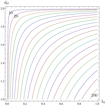
Figure 1 (2) shows the possible values of $(\lambda_{0},d_{\cal U})$ for various Higgs (light scalar) masses. One can see that heavier scalars constrain $d_{\cal U}$ more strongly. Thus the discovery of, say, Higgs alone of mass $\lesssim 400$ GeV will not give much information on $d_{\cal U}$.

As also given in Fig. 3, $m_{h}$ is rather inert with respect to $d_{\cal U}$ while $m_{\ell}$ is not. With the condition of Eq. (28), both $m_{h,\ell}$ are proportional to $\sim\sqrt{\lambda_{0}}$. One can find that

for $d_{\cal U}=1(2)$. As $d_{\cal U}$ increases $m_{h}$ increases slightly while $m_{\ell}$ decreases and finally vanishes at $d_{\cal U}=2$, and the gap between $m_{h}$ and $m_{\ell}$ gets larger as $d_{\cal U}$ increases. If the scalar masses turned out to be quite different from Eq. (29), then the value of $\mu$ should be rearranged to fit the data. But in this case one would have to explain why that value of $\mu$ is so different from $v_{0}$, the electroweak scale.

Conclusions.— In this Letter we suggest a new scalar potential with a fractional power of fields from hidden sector inspired by the scalar unparticle operator. Unlike the usual potential of marginal coupling, the new one develops VEV at tree level. In this picture, the EWSB occurs when the unparticle sector begins to interact with the SM sector. If the hidden sector were not scale invariant and the coupling were marginal, the EWSB happens radiatively through the CW mechanism. When the scaling dimension $d_{\cal U}$ departs from the value of $2$ a new scale (of the order of $\sim 1/\sqrt{G_{F}}$) is introduced in the scalar potential through the relevant coupling, and the electroweak symmetry is broken at tree level. In other words, the EWSB occurs when the hidden sector enters the regime of scale invariance, i.e., unparticles. In view of the unparticle sector, the new potential also breaks the scale invariance of the hidden sector.

Once the electroweak symmetry is broken, the scalar fields from SM and hidden sector mix together to form two massive physical states. The heavy one is identified as Higgs, while the light one is a new particle of mass around $\lesssim 230$ GeV. The possibility of the new light scalar to be a dark matter will be a good challenge for future studies.

If the hidden sector self coupling $\lambda_{1}$ vanishes, then the minimum of the potential appears along the ray of $\Phi=0$. In this case the VEV cannot produce the $W$ boson mass $m_{W}$ since $m_{W}$ occurs when the fluctuation is transverse to the $\Phi=0$ direction. Thus our potential $V(\Phi,\phi)$ in Eq. (3) is minimal.

References

- [1] K. A. Meissner and H. Nicolai, Phys. Lett. B 648, 312 (2007) [arXiv:hep-th/0612165].
- [2] J. R. Espinosa and M. Quiros, Phys. Rev. D 76, 076004 (2007) [arXiv:hep-ph/0701145].
- [3] W. F. Chang, J. N. Ng and J. M. S. Wu, Phys. Rev. D 75, 115016 (2007) [arXiv:hep-ph/0701254].
- [4] R. Foot, A. Kobakhidze and R. R. Volkas, Phys. Lett. B 655, 156 (2007) [arXiv:0704.1165 [hep-ph]].
- [5] S. R. Coleman and E. Weinberg, Phys. Rev. D 7, 1888 (1973).
- [6] H. Georgi, Phys. Rev. Lett. 98, 221601 (2007) [arXiv:hep-ph/0703260]; Phys. Lett. B 650, 275 (2007) [arXiv:0704.2457 [hep-ph]].
- [7] K. Cheung, W. Y. Keung and T. C. Yuan, Phys. Rev. Lett. 99, 051803 (2007) [arXiv:0704.2588 [hep-ph]], Phys. Rev. D 76, 055003 (2007) [arXiv:0706.3155 [hep-ph]]; M. Luo and G. Zhu, Phys. Lett. B 659, 341 (2008) [arXiv:0704.3532 [hep-ph]]; Y. Liao, Phys. Rev. D 76, 056006 (2007) [arXiv:0705.0837 [hep-ph]]; T. Kikuchi and N. Okada, arXiv:0707.0893 [hep-ph]; A. Lenz, Phys. Rev. D 76, 065006 (2007) [arXiv:0707.1535 [hep-ph]]; J. R. Mureika, Phys. Lett. B 660, 561 (2008) [arXiv:0712.1786 [hep-ph]]; B. Grinstein, K. Intriligator and I. Z. Rothstein, arXiv:0801.1140 [hep-ph].
- [8] P. J. Fox, A. Rajaraman and Y. Shirman, Phys. Rev. D 76, 075004 (2007) [arXiv:0705.3092 [hep-ph]].
- [9] A. Delgado, J. R. Espinosa and M. Quiros, JHEP 0710, 094 (2007) [arXiv:0707.4309 [hep-ph]].
- [10] M. A. Stephanov, Phys. Rev. D 76, 035008 (2007) [arXiv:0705.3049 [hep-ph]].
- [11] J. P. Lee, arXiv:0710.2797 [hep-ph].
- [12] E. Gildener and S. Weinberg, Phys. Rev. D 13, 3333 (1976).
- [13] W. D. Goldberger, B. Grinstein and W. Skiba, arXiv:0708.1463 [hep-ph].