Transport in suspended graphene
Abstract
Motivated by recent experiments on suspended graphene showing carrier mobilities as high as , we theoretically calculate transport properties assuming Coulomb impurities as the dominant scattering mechanism. We argue that the substrate-free experiments done in the diffusive regime are consistent with our theory and verify many of our earlier predictions including (i) removal of the substrate will increase mobility since most of the charged impurities are in the substrate, (ii) the minimum conductivity is not universal, but depends on impurity concentration with cleaner samples having a higher minimum conductivity. We further argue that experiments on suspended graphene put strong constraints on the two parameters involved in our theory, namely, the charged impurity concentration and , the typical distance of a charged impurity from the graphene sheet. The recent experiments on suspended graphene indicate a residual impurity density of which are presumably stuck to the graphene interface, compared to impurity densities of for graphene on SiO2 substrate. Transport experiments can therefore be used as a spectroscopic tool to identify the properties of the remaining impurities in suspended graphene.
pacs
81.05.Uw; 72.10.-d, 73.40.-cI Introduction
The recent experimental realization of a single layer of carbon atoms arranged in a honeycomb lattice has prompted much excitement in both theoretical and experimental physics communities (For a recent review, see Ref. 1 and references therein). Most experiments so far have been performed on a SiO2 substrate using the mechanical exfoliation technique developed in Ref. 2 followed by optical detection that is sensitive to the thickness of the substrate. In these experiments one expects there to be charged impurities located in the substrate with a typical density of with the impurities sitting near the substrate-graphene interface with a typical distance from the graphene sheet. In previous work [4, 3] we argued that removing the substrate would remove the charged impurities and enhance mobility. Other models of scattering such as ripples, on the other hand, would lead to enhanced scattering in suspended graphene thereby reducing the mobility, since a freely suspended graphene sheet is expected to be more rippled than one glued to a substrate.
Very recently experiments have been performed on suspended graphene [5, 6] that find remarkably high mobilities for carrier transport confirming that charged impurities in the substrate were indeed the dominant scattering mechanism limiting the mobility. Signatures from these new experiments (such as the conductivity still being linear in carrier density) imply that the remaining impurities in suspended graphene are long-range and are probably charged dopants lying (i.e. stuck) on the graphene surface, or remnants of chemicals used during the preparation. The minimal model we propose here contains only two parameters: the charged impurity density and the typical distance of the impurity from the graphene sheet. Theoretical estimates for these numbers in suspended graphene are hard to come by, for example, a recent DFT study [7] argues that potassium and sodium dopants are typically located at from a graphite surface. In what follows we treat and as parameters, and argue that the experimental signatures both at high density and low density effectively constrain these numbers. Turning the problem around, the recent transport experiments on suspended graphene could be used as a spectroscopic tool to identify the properties of the remaining impurities in suspended graphene. For example, a mobility , implies that , or equivalently, that the distance between the remaining impurities is around with the charged impurities sitting typically at an effective distance of from the graphene sheet.
II Theoretical Model
To calculate the transport properties of graphene, we consider impurities with an effective density located in a plane at a distance , either above or below the graphene sheet. While in reality, different impurities may be located at different distances, one should therefore think of as an effective or typical impurity distance and as an average 2D impurity density. Alternatively, one could imagine several impurity planes at different distances , and then adding up their respective contributions to conductivity using Matthiessen’s rule. As we show below, impurities located farther away are exponentially suppressed, so in this respect, one could then think of then as distance of the closest charged impurities and thus dominating the transport properties. In any case, our minimal model for charged impurities contains only two parameters and .
For an impurity located at the origin, the bare Coulomb potential at the point in the graphene sheet is
| (1) |
where is the impurity charge and is an effective background lattice dielectric constant. All the properties of the substrate (or vacuum in the case of suspended graphene) can be absorbed into a third parameter , where . Here is the speed of light, and is the constant graphene Fermi velocity that relates energy to momentum in the linear Dirac spectrum . The carrier density . Although we keep as an arbitrary number in the theory, we note for concreteness that for graphene on a Si02 substrate, and for suspended graphene (see Refs. 3, 4 for further details on the model). The Fourier transform of Eq. 1 gives
| (2) |
where in the second line, we assume linear screening with
| (3) |
Although our choice of dielectric function has an artificial discontinuity at , its advantage is that it allows for analytic results, and we have checked by numerical integration that this choice of dielectric function and the Random Phase Approximation [9, 8] give identical results for all graphene transport properties (see Ref. 3 and references therein for a discussion of this point). Further, we observe that the chiral properties induced by the sub-lattice structure of the honeycomb lattice imply that in contrast to most other electronic systems, scattering is absent in graphene.
Graphene conductivity can then be calculated in Boltzmann transport theory where and
where is the spinor component of the electron (or hole) eigenvector of the Dirac Hamiltonian. These expressions can be simplified by introducing two dimensionless variables and to find
| (4) |
To calculate the transport properties of graphene from Coulomb impurities the integral was solved numerically by Ando [9], Cheianov and Falko [10] and Hwang et al [4]. We explore several limits in which can be solved analytically. In the “Complete Screening” limit, , Nomura and MacDonald [11] showed that . This result does not capture the effect of changing the substrate which in turn changes the parameter . This complete screening approximation is therefore inadequate to study transport in suspended graphene even at a qualitative level. For example, as we show below, keeping the same, but just changing the dielectric constant from SiO2 to vacuum, would actually decrease mobility by almost a factor of 2. Therefore, in suspended graphene the two effects of reducing both dielectric constant and actually compete to determine graphene mobility (see also Ref. 12). Taking , but keeping the dependence, we showed [3] that
| (5) |
We note here that the following additional limits can be solved: , where is a modified Bessel function and is a modified Struve function. We also have , where this last result says that for very large density, Coulomb impurities in graphene give . However, this is not the limit relevant to experiments, which are all in the low density regime. The following expansion captures both the substrate (i.e. dependence) and the dependence, and is relevant for current experiments both on suspended graphene and for graphene on a SiO2 substrate
| (6) |
where
| (7) |
We note that for most relevant substrates , (recall that for a SiO2 substrate and for suspended graphene ), and that the ratio does not change significantly from its large asymptote of . Therefore for practical comparisons with experiments, one can approximate graphene conductivity using
| (8) |
For SiO2 substrate , giving the result of , and for suspended graphene, giving . We find Eq. 8 to be a very useful formula for all existing bulk graphene transport data in the literature.
We now turn to the discussion of mobility . Defining mobility in graphene is both important and problematic. The importance stems mostly from it being the figure of merit for graphene’s application as a practical transistor device. However, close to the Dirac point we have but finite resistivity. If one naively assumes that in this regime as is often done, then one can get arbitrarily high values of mobility which is completely meaningless (a detailed discussion of this point can be found in Ref. 13). Calculating mobility at very high density is complicated by the fact that both super-linear contributions (see Eq. 6 for finite ) and sub-linear contributions from short-range scatterers (see Ref. 3, 4 and discussion in Sect. IV below) come into play, so that mobility is not constant for a given sample. In this case, mobility would be a non-monotonic function of carrier density whose maximum value is given by a competition of different scattering mechanisms present in graphene. We have consistently argued that the best definition of graphene mobility is the slope just beyond the Dirac point conductivity plateau, i.e. only within the window of density where the conductivity is strictly linear in . We advocate this choice because at low density, one can show theoretically that both the sub-linear and super-linear contributions to the conductivity are small. For this definition of mobility, one can immediately see that
| (9) |
where . Although our theory has two free parameters, i.e. and , knowing the mobility immediately determines through Eq. 9. A careful characterization of the super-linear contribution using Eq. 6 could then be used to determine . In addition, as we describe below, the low density transport properties i.e. the value of the minimum conductivity, the width of the minimum conductivity plateau and the offset of the Dirac point depend only on these two parameters that in principle could already be determined from the high-density transport data.
So far we have formulated everything in terms of carrier density . For large external gate voltage, we can map our results to applied gate voltage using , where is experimentally determined to be for graphene on SiO2 and for suspended graphene [14, 5]. The last step is to determine the carrier density close to the Dirac point. The low density conductivity arises from the carriers in the charge-impurity induced puddles of electrons and holes [4]. We argued in Ref. 3 that at low density it was appropriate to use the rms density caused by the inhomogeneous potential induced by the same charged impurities that are responsible for the high-density transport properties. A self-consistent calculation gives [3]
| (10) | |||||
where is the exponential integral function and the self-consistency is obtained by setting . The offset in the Dirac point is given by (a derivation of this result can be found in Ref. 3). The value of calculated from this self-consistent calculation agrees with a recent calculation that minimizes the graphene energy functional in the presence of disorder [15] and for is consistent with the experimental observations of density inhomogeneities on a SiO2 substrate [16]. Given the choice of substrate (which determines ) and picking and completely determines the conductivity at high density and the non-universal disorder dependent minimum conductivity plateau at low density.
III Results
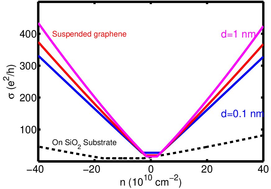
To illustrate our results, in what follows, we choose the experimental parameters reported in Ref. 5. We use mobility for graphene on a substrate (corresponding to ) and for suspended graphene (). We also employ a hard cut-off between the low and high density regime such that if and for . Shown in Fig. 1 is the resistivity as a function of gate voltage for both suspended graphene and graphene on a SiO2 substrate. An important observation is that the higher mobility samples have a lower resistivity which is an important prediction of our self-consistent theory [3]. This has been verified both in transport measurements on SiO2 substrate [14] and by intentionally adding charged impurities in ultra-high vacuum [17]. The recent data [5] on ultra-high mobility suspended graphene samples further confirm that charged impurities provide the dominant scattering mechanism in graphene and are responsible for the non-universal minimum conductivity. We note that in plotting resistivity, all the super-linear behavior is obscured and the high-density curves of the same mobility but different look quite similar. By contrast, from the properties of the low density “Dirac plateau” one can extract the magnitude of , but we caution that we only expect our self-consistent carrier density theory to agree within a factor of two with the experimentally observed plateau width, Dirac point offset and the maximum resistivity. A careful analysis of the experimental data should be able to extract the best values for and as has been done previously for graphene on a substrate [14, 17].

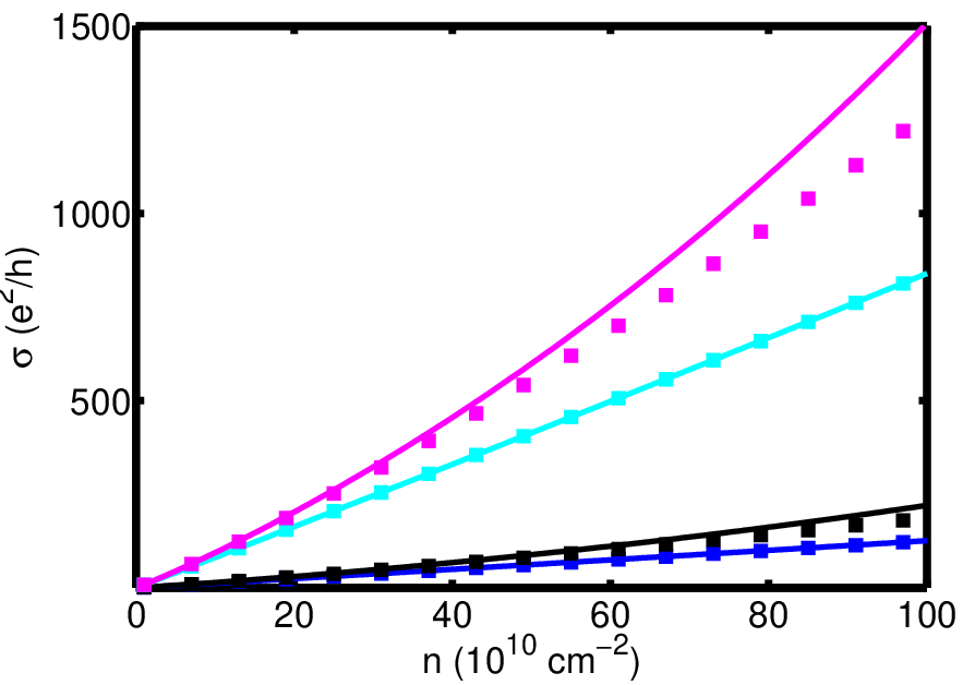
In Fig. 2 we show conductivity as a function of “carrier density” defined through . For experimentally reasonable carrier densities, one can notice that and should be distinguishable by the super-linear contributions of the former. In many ways plotting the data as conductivity instead of resistivity reveals much more information. From these results we argue that transport data not only provide information about but also , thereby being a tool to not only identify different types of scattering mechanisms (e.g. short-range, long-range, phonons) but for Coulomb impurities, it provides information about the location of the impurities. In Fig. 3 we show our analytical expression Eq. 6 (solid lines) compared to a numerical evaluation of Eq. 4 (squares) for different values of and for both suspended graphene and on a substrate. One finds that for most of the experimental regime, the analytical expression is an excellent approximation for the Boltzmann conductivity, but that at very high-density and large , it slightly over-estimates the super-linear behavior. However, in this high-density regime, one also expects the contribution of non-Coulombic short-range scatterers which reduce the conductivity. For large and a particular ratio of short-range and Coulomb scatterers, one may even have non-monotonic mobility that first increases because of our predicted super-linear contribution and then decreases as short-range scattering becomes more dominant at higher densities.
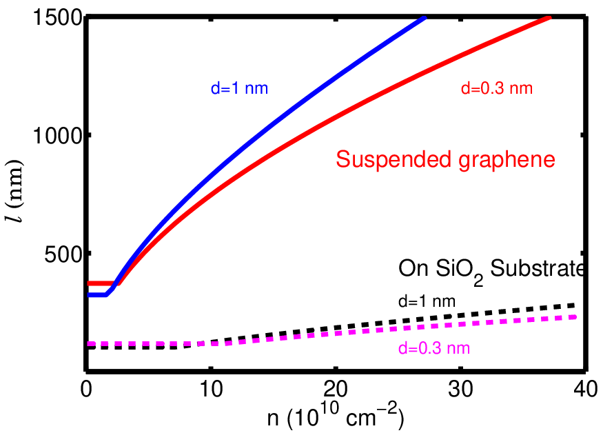
Finally, in Fig. 4, we show our calculated carrier mean free path () as a function of carrier density, comparing graphene on SiO2 substrate with suspended graphene. It is remarkable that, for reasonable parameters (same as Fig. 1) used in these results, the suspended graphene for whereas for the same density range in graphene on SiO2 substrate, the charged impurities give rise to an almost constant . As noted by Bolotin et al. [5] such long () mean free paths are comparable to the 2D system size of the samples, implying ballistic transport and a breakdown of our diffusive theory. It is important to realize that for mean free paths comparable to the sample size, strong short-range scattering will be imposed by the sample edges leading to a saturation of the conductivity and the mean-free-paths around this density. Note, however, that the current graphene samples on the substrate are always in the diffusive limit, and graphene transport around the Dirac point (both with and without substrate) is also always in the diffusive limit since the mean free path is much shorter than the sample size. Of course, by making nanoribbons [19, 18] with sample sizes comparable to , one can artificially induce ballistic transport.
IV Discussion
In this work, we have generalized the transport theory of Ref. 3 to the case of suspended graphene [5] and derived analytical results for the super-linear contribution to conductivity expected for Coulomb scatterers at a finite distance from the graphene sheet. However, this effect becomes pronounced only at high density where short-range scattering begins to dominate over Coulomb scattering. We note that in the experiments of Bolotin et. al [5], they were only able to reach rather low carrier densities, and therefore we believe that Coulomb scattering dominates over all other scattering mechanisms in their results. However, as was pointed out in Ref. 5, there may be strong short-range scattering by sample edges when the mean free path becomes comparable to the system size. However one can anticipate for the Dirac plateau in cleaner samples (such as future suspended graphene experiments), charged impurities will induce a smaller carrier density , even as the ratio is increasing. For example, a sample with mobility of , would have which for gives and . This gives . So despite the high-mobility, the peculiar scaling for Coulomb scatterers in graphene implies that close to the charge neutral point, we are in the diffusive Boltzmann transport regime. However, at higher carrier density we have , suggesting that the ballistic regime could be explored away from the Dirac point. For mesoscopic samples constructed in the geometry of , where is the sample size, our theory does not apply.
Smaller sample sizes would also increase the effect of edge scattering, which act as short-range scattering centers. As was argued in Hwang et al. [4] at high density these begin to dominate showing a non-universal cross-over from the low-density regime where is linear in to the high-density limit where is constant. So while in this work we have focused on Coulomb scattering that dominates at low density, probing a wider density range could also distinguish between different scattering mechanisms. We emphasize here that detailed measurements and analysis of could thus provide in-depth spectroscopic information about the impurity distribution in graphene, far surpassing the resolution of currently available scanning microscopy measurements [16] which directly probe the potential landscape.
Finally we note that alternative theories for the dominant scattering mechanism in graphene make predictions that are inconsistent with the results of Bolotin et al. [5]. For example, if ripples were the dominant scattering mechanism, then suspended graphene would have stronger ripples and hence lower mobility. It was one of our early predictions that removing charged impurities in the substrate would increase mobility and increase the minimum conductivity. The initial conventional wisdom in the theoretical community that graphene experiments were observing the universal Dirac minimum conductivity should now be discarded after recent experimental developments including intentionally doping graphene with potassium in Ref. 17 and measurements done on graphene with mobility varying close to three orders of magnitude in Refs. 14, 5 and most particularly the suspended graphene measurements, all of which clearly demonstrate the importance of charged impurity disorder controlling the minimum conductivity plateau. It was in Refs. 4, 3 that we predicted that charged impurities in graphene would give rise to a non-universal minimum conductivity whose value would increase with cleaner samples. These predictions have now been vindicated in light of recent experiments. It, therefore, appears that the existing graphene transport experiments are completely dominated by charged impurity scattering, and no universal “Dirac point physics” is in play near the charge neutrality point. The physics of the charge neutrality point is dominated by diffusive transport through electron and hole puddles induced by the charged impurities. We believe that the close agreement between our theory and the transport data in suspended graphene experiments establishes the dominance of charged impurity scattering in graphene beyond any reasonable doubt.
This work is supported by U.S. ONR and NSF-NRI.
References
- [1] S. Das Sarma, A. K. Geim, P. Kim, and A. H. MacDonald, eds., Exploring Graphene: Recent Research Advances, A Special Issue of Solid State Communications, vol. 143 (Elsevier, 2007).
- [2] K. S. Novoselov, A. K. Geim, S. V. Morozov, D. Jiang, Y. Zhang, S. V. Dubonos, I. V. Grigorieva, and A. A. Firsov, Science 306, 666 (2004).
- [3] S. Adam, E. H. Hwang, V. M. Galitski, and S. Das Sarma, Proc. Natl. Acad. Sci. USA 104, 18392 (2007).
- [4] E. H. Hwang, S. Adam, and S. Das Sarma, Phys. Rev. Lett. 98, 186806 (2007a).
- [5] K. Bolotin, K. Sikes, Z. Jiang, G. Fudenberg, J. Hone, P. Kim, and H. Stormer, arXiv:0802.2389v1 (2008).
- [6] X. Du, I. Skachko, A. Barker, and E. Andrei, arXiv:0802.2933v1 (2008).
- [7] K. Rytkönen, J. Akola, and M. Manninen, Phys. Rev. B 75, 075401 (2007).
- [8] E. H. Hwang and S. Das Sarma, Phys. Rev. B 75, 205418 (2007).
- [9] T. Ando, J. Phys. Soc. Jpn. 75, 074716 (2006).
- [10] V. Cheianov and V. Fal’ko, Phys. Rev. Lett. 97, 226801 (2006).
- [11] K. Nomura and A. H. MacDonald, Phys. Rev. Lett. 96, 256602 (2006).
- [12] J. Sabio, C. Seoanez, S. Fratini, F. Guinea, A. H. Castro Neto, and F. Sols, arXiv:0712.2232v3 (2007).
- [13] E. H. Hwang, S. Adam, and S. Das Sarma, Phys. Rev. B 76, 195421 (2007b).
- [14] Y.-W. Tan, Y. Zhang, K. Bolotin, Y. Zhao, S. Adam, E. H. Hwang, S. Das Sarma, H. L. Stormer, and P. Kim, Phys. Rev. Lett. 99, 246803 (2007).
- [15] E. Rossi and S. Das Sarma, Preprint (2008).
- [16] J. Martin, N. Akerman, G. Ulbricht, T. Lohmann, J. H. Smet, K. von Klitzing, and A. Yacobi, Nature Physics 4, 144 (2008).
- [17] J. H. Chen, C. Jang, S. Adam, M. S. Fuhrer, E. D. Williams, and M. Ishigami, Nature Physics, in press (arXiv:0708.2408v1) (2008).
- [18] M. Y. Han, B. Ozyilmaz, Y. Zhang, and P. Kim, Phys. Rev. Lett. 98, 206805 (2007).
- [19] F. Miao, S. Wijeratne, Y. Zhang, U. Coskun, W. Bao, and C. Lau, Science 317, 1530 (2007).